DSGE Model-Slovakia

Full text

(1)Juraj Zeman, Matúš Senaj. DSGE MODEL - SLOVAKIA. Working paper 3/2009.

(2) © National Bank of Slovakia http://www.nbs.sk/ Imricha Karvaša 1 813 25 Bratislava research@nbs.sk. May 2009. ISSN: 1337-5830. The views and results presented in this paper are those of the authors and do not necessarily represent the official opinion of the National Bank of Slovakia. All rights reserved..

(3) Working paper 3/2009. DSGE model - Slovakia Juraj Zeman, Matúš Senaj Research Department, National Bank of Slovakia juraj.zeman@nbs.sk matus.senaj @nbs.sk. Abstract DSGE Slovakia is a medium size New Keynesian open economy model designed to simulate dynamic behavior of Slovak economy. It consists of about 50 equations and contains all important macroeconomic variables including real GDP and all its main components- consumption, investment, government expenditures, import and export then factors of production – labor, capital and oil and also consumer, producer, import and export price deflators, nominal interest rate and exchange rate. Most parameters of the model are calibrated and remaining ones are estimated by various estimation technique. Appropriateness of the model is judged by comparing statistics of simulated data with real ones, by analyzing impulse response functions and by reproducing historical time series.. Keywords: General equilibrium model, Slovakia JEL classification: D58, E32 Reviewed by: Jean-Marc Natal (Swiss National Bank) Michal Horváth (University of Oxford) Downloadable at http://www.nbs.sk/.

(4) DSGE MODEL - SLOVAKIA. 1 Introduction In this paper we present a DSGE model for the Slovak economy. The key features of DSGE models are microeconomic foundations of their equations, rational expectations of all economic agents involved and a general equilibrium setting. These features ensure a theoretical cohesion of the model and make it suitable predominantly for qualitative analysis - studying different stages of business cycles, analyzing impacts of various policy changes as well as responses of variables to various structural shocks. The first simple versions of DSGE models, however, were trailing behind more empirically based models (e.g. VARs) in capturing empirical properties of real economy. In order to improve empirical tractability of DSGE models, simple versions were augmented by including more variables and by introducing various frictions. These enhanced DSGE models are comparable and in many instances even outperform their empirically based counterparts in empirics (Smets and Wouters, 2003) and can be used also for forecasting purposes. Model presented in this paper is based on the work of Cuche-Curti, Dellas and Natal: DSGE model for Switzerland1. It is a medium size New Keynesian small open economy model designed to simulate dynamic behavior of Slovak economy. It consists of about 50 equations and contains all important macroeconomic variables including real GDP and all its main components- consumption, investment, government expenditures, import and export then factors of production – labor, capital and oil also consumer, producer, import and export price deflators, nominal interest rate and exchange rate. The model displays sticky nominal prices and wages that adjust to staggered price/wage setting a la Calvo. In order to improve the persistence of inflation a partial indexation scheme for non-optimizers is introduced. The model also incorporates capital adjustment cost (paid for transforming investment into capital) which smoothes investment and external habit formation (“catching up with Jonses”) that improves consumption dynamics. Here we present first version of the model, the so called “baby model”, which will be extended and improved in the near future. The structure of the paper is as follows. Next section introduces main features of the model. Section 3 provides detailed description of the behavior of all agents in the modeled economy, such as firms, households, government and the central bank. The method of calibration of the parameters is described in section 4. Finally, section 5 presents the impulse response 1. Authors thank to Jean-Marc Natal for his permission to use their model as a benchmark and for his invaluable help. National Bank of Slovakia Working paper 3/2009. 4.

(5) DSGE MODEL - SLOVAKIA. functions of the model. Particularly, we study four shocks: monetary policy loosening, expansionary fiscal policy, productivity shock and oil price shock.. 2 Main features Equation Section (Next)Equation Section (Next) The model has the following structure: Production There are two sectors of production – intermediate goods and final goods. Inputs for intermediate goods are labor, capital and oil. Intermediate goods are tradable and can be used either domestically for producing final goods or can be exported abroad. Producers in this sector produce differentiated good. There is imperfect competition in this sector and hence producers have market power in setting price of goods used domestically (Kollmann, 2002). Final goods are produced of intermediate goods either domestic or imported and of oil and are either consumed privately, publicly or invested. There is perfect competition in final good production sector. Final good is non tradable. Household There is a representative household who maximizes lifetime utility out of consumption and leisure. She makes two decisions: current consumption vs investment (that gives her higher consumption in future) and hours worked vs leisure. There is imperfect competition in the labor market that gives market power to workers in wage setting. In order to improve dynamics of the model, household sector is enhanced with the following amendments: habit formation in consumption (Fuhrer, 2000) which ensures that consumers smooth their consumption, fraction of consumers who do not borrow or save but instead spend all their current labor income (rule-of-thumb consumers, Gali et al, 2004) and capital adjustment costs that implies the cost of transforming investment into capital. Trade Only intermediate goods can be traded. Domestic firms export a fraction of intermediate goods abroad. Prices of exported intermediate goods can differ from prices of intermediate goods sold domestically (pricing to market structure – Bergin, Feenstra, 1999). Imported intermediate goods can not be consumed directly. Importing firms have market power in setting price of import. Hence exchange rate pass-through is incomplete and the law of one price does not necessarily hold in short term (Monacelli, 2005). National Bank of Slovakia Working paper 3/2009. 5.

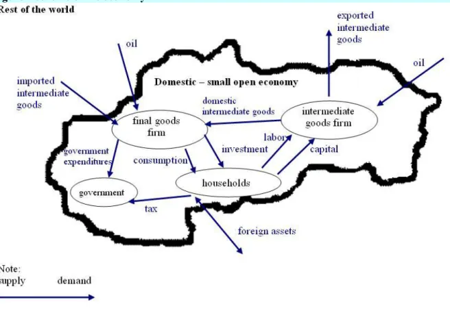
(6) DSGE MODEL - SLOVAKIA. Financial market Financial market is incomplete. In equilibrium, foreign investors do not hold domestic bonds. This means that the amount of domestic bonds equals zero at all times. Economies with incomplete insurance against idiosyncratic shocks have the potential to account for low correlation of consumption between domestic and foreign countries, the pattern that is observed in data (Backus et al, 1995). Domestic agents can insure against shocks by holding foreign assets. To avoid of excessive accumulation of net foreign assets in domestic economy in the model, their price increase with their level. The more is domestic country indebted (higher level of net foreign assets), the costlier for its citizens is to borrow further. Monetary and fiscal policy Monetary authority reacts to deviations of inflation, output and exchange rate from their steady state values by setting nominal interest rate (Taylor rule). Fiscal authority keeps balanced budget each period. Price setting There is staggered price setting á la Calvo for the prices of domestic and imported intermediate goods as well as for the price of labor (wages). Firms (workers) can not change their price unless they receive a random “price-change signal”. If it does not receive this signal the price is automatically adjusted according to certain indexation scheme. Exogenous shocks There are several domestic and external shocks in the model. Domestic shocks are to productivity, fiscal expenditure and domestic interest rate. External shocks are to foreign output, foreign interest rate, foreign price level and to oil price.. National Bank of Slovakia Working paper 3/2009. 6.

(7) DSGE MODEL - SLOVAKIA. Figure 1 scheme of the economy. Trends vs cycles It is assumed that all real variables including output and its components are non-stationary processes with common stochastic trend. Hence all these variables are transformed to stationary ones by taking this stochastic trend away (de-trended) before they enter the model. Price deflators are assumed to be non-stationary processes with common stochastic trend. Original non-stationary deflators are denoted by upper case letters (Pt) while their corresponding de-trended counterparts are denoted by lower case letters (pt). All other variables including interest rate and exchange rate are assumed to be stationary. A “hat” on a variable indicates the percentage deviation of that variable from its steady state value. In the case of net inflation and net interest rate, “hat” indicates difference of that variable from steady state value. The final version of the model consists of a set of equations some of which are linearized by hand and remaining are left non-linear. The model is solved numerically using DYNARE software package2 developed by Michel Juillard.. 2. DYNARE is downloadable at http://www.cepremap.cnrs.fr/juillard/mambo/index.php. National Bank of Slovakia Working paper 3/2009. 7.

(8) DSGE MODEL - SLOVAKIA. 3 The model 3.1 Final goods firms Final goods firms operate in a perfectly competitive market and produce non-tradable goods d. from a bundle of domestic intermediate goods ( xt ), a bundle of imported intermediate goods m. ( xt ) and energy ( et ). Final goods are either consumed by domestic households ( ct ) and government ( g t ) or invested domestically ( it ). Figure 2 final goods firm. xdt Pdt. xmt Pmt. et Pet. Final goods firm. ct Pct. it Pit. gt Pgt. These different types of final goods l Î {c, i, g } , whose demand is determined in a household sector, are produced with a technology represented by the production function. [. 1- r e ,l. l t = w e ,l. a ( x tl ). r e ,l. + (1 - w e ,l ). 1- r e , l. (etl ). re ,l. ]. 1/ r e , l. (3.1). with. [. a( xtl ) = wl1- rl ( xtd ,l ) rl + (1 - w l )1- rl ( xtm,l ) rl. ]. 1 / rl. (3.2). Aggregator a( ) combines domestic and imported intermediate goods with elasticity of substitution between them equal to (1/1 - rl ) . wl is the share of domestic intermediate goods in the bundle. Then the bundle of intermediate goods is combined with energy and final goods are produced. The elasticity of substitution between intermediate goods and energy is. (1 /1 - r ) and the share of energy is ( 1 - w e ,l. National Bank of Slovakia Working paper 3/2009. e ,l. ). Notice that elasticity of substitution between 8.

(9) DSGE MODEL - SLOVAKIA. the bundle of intermediate goods and energy is in general different (much smaller, of course) from the elasticity of substitution between intermediate goods themselves. Final goods firms optimize their production by minimizing their total cost. Given the price of domestic intermediate goods - Pt d , the price of imported intermediate goods - Pt m and the price of energy - Pt e , they solve the following problem min TCt =. {. min. xtd ,l , xtm ,l ,etl. ì Pt d xtd ,l + Pt m xtm ,l + Pt e etl + y tl ílt } î. - éëw. 1- re ,l e ,l. l r e ,l t. a( x ). 1- re ,l. + (1 - we,l ). l re ,l t. (e ). ù û. 1/ re ,l. ,. ü ý þ. (3.3). l Î {c, i, g } . y tl is a Lagrange multiplier that represents marginal cost. Solution to this problem leads to following demand functions: x. x. d ,l t. m ,l t. 1. æ Pt d = çç l è Pt. ö rl -1 ÷÷ w l a ( xtl ) ø. æ Pm = çç t l è Pt. ö rl -1 ÷÷ w l a ( xtl ) ø. 1. æ Pe etl = çç t l è Pt. re , l - rl 1- r l. 1- r e ,l. (w e,l lt ) 1- rl (3.4). r e ,l - r l 1- r l. 1- r e ,l. (w e,l lt ) 1- rl (3.5). 1. ö re ,l -1 ÷÷ (1 - w e,l )lt ø. (3.6). Value of a( xtl ) at the optimal quantities is 1- rl. rl rl r l (1- re ,l ) é d r -1 m r -1 ù l l æ ö æ ö P P a( xtl ) = we,l lt êwl ç t l ÷ + (1 - wl ) ç t l ÷ ú ê ú è Pt ø è Pt ø ú ëê û. (3.7). By substituting these optimal quantities into total cost (TCt) we can get the expressions for marginal costs y tl . Because final goods firms operate in a perfectly competitive market,. marginal cost equals price level, y tl = Pt l , l Î {c, i, g } . ì ï é Pt = íw e ,l êwl Pt d ï ë î l. ( ). rl r l -1. rl m r -1 l. ( ). + (1 - w l Pt. r e ,l (1- r l ). ù rl (1- r e ,l ) + (1 - w e ,l ) Pt e ú û. ( ). ü ï r e ,l -1 ý ï þ r e ,l. r e ,l -1 r e ,l. (3.8). Bundles xtd ,l and xtm ,l are CES aggregators of domestic and imported intermediate goods produced by i firms, i Î [0,1]. National Bank of Slovakia Working paper 3/2009. 9.

(10) DSGE MODEL - SLOVAKIA 1. xtd ,l 1 1- qd goods.. æ 1 çç è1-qm. æ1 ö qd = çç ò xtd ,l (i)q d di ÷÷ è0 ø. 1. and. xtm,l. æ1 ö qm = çç ò xtm ,l (i )q m di ÷÷ è0 ø. (3.9) (3.10). ö ÷÷ is the elasticity of substitution between domestic (imported) intermediate ø. The aggregator chooses the bundle of goods that minimizes the cost of producing a given quantity xtd ,l , ( xtm ,l ) taking the prices Pt d (i ) , ( Pt m (i ) ) as given. This leads to the following demand functions for goods i 1. æ P d (i ) ö q d -1 d ,l xtd ,l (i ) = çç t d ÷÷ xt è Pt ø. 1. and. æ P m (i) ö q m -1 m,l xtm,l (i ) = çç t m ÷÷ xt è Pt ø. (3.11) (3.12). where Pt d and Pt m are unit costs of the bundles xtd ,l and xtm ,l respectively, given by æ 1 d qq d-1 ö d Pt = ç ò Pt (i ) d di ÷ ÷ ç0 è ø. q d -1 qd. and. æ 1 m qq m-1 ö m Pt = ç ò Pt (i) m di ÷ ÷ ç0 è ø. qm -1 qm. (3.13) (3.14). We can interpret Pt d and Pt m as the aggregate price indices.. 3.2. Intermediate goods firms. Each domestic intermediate firm produces a differentiated good xt (i ) with capital k t (i ) , x. labor ht (i ) and energy et (i ) which is then used domestically - xtd (i) for producing final goods or exported - xtf (i ) , xt (i) = xtd (i ) + xtf (i). Figure 3 intermediate goods firm. kt(i) zt. ext(i) Pet. ht(i) wt. ith Intermediate goods firms. xdt(i). xft(i). Pdt(i). Pft(i). National Bank of Slovakia Working paper 3/2009. firm. 10.

(11) DSGE MODEL - SLOVAKIA. Production function for intermediate good i is a CES function 1 s e -1 ìï s1 k ,l se e s xt (i ) = At ía c xt (ht (i ), k t (i ) e + (1 - a c ) etx (i) ïî. [. ]. (. se. s e -1 se. ). üï s e -1 ý ïþ. (3.15). with 1 s k ,l -1 s k ,l -1 ü ìï s1 ï s k ,l k ,l x (ht (i ), kt (i )) = ía l ( ht (i) ) s k ,l + (1 - a l ) ( kt (i ) ) s k ,l ý îï þï. s k ,l s k ,l -1. k ,l t. ,. (3.16). where At represents an exogenous stationary stochastic technological shock. s k ,l is elasticity of substitution between labor and capital and s e is elasticity of substitution between labor/capital and energy. Each firm i tries to minimize total cost of producing xt (i) intermediate goods demanded by domestic and foreign final goods producers. Given wage rate wt , rental rate of capital zt and the price of energy Pt e , firm i solves the following problem min TCt (i ) =. ìï wt ht (i) + zt kt (i) + Pt e etx (i ) + y t (i) í xt (i ) {ht (i ), kt (i ),et (i )} ïî min x. 1 s e -1 ìï s1 k ,l se e s - At ía c éë xt (ht (i), kt (i ) ùû e + (1 - a c ) etx (i ) ïî. (. ). s e -1 se. (3.17). se ü üïs e -1 ï ý ý ïþ ï þ. where y t (i ) is marginal cost of a firm i. The solution to this problem implies that all firms have identical real marginal cost y t that does not depend on i 1 yt = At. [. ì 1-s k ,l 1-s + (1 - a l ) z t k ,l ía c a l wt î. ]. s e -1 s k , l -1. 1. ü 1-s e + (1 - a c )( Pt e )1-s e ý þ. (3.18). Then index i can be dropped and we get aggregate demand for labor, capital and energy. [. x -s 1-s 1-s ht = a ca l t (y t At )s e wt k ,l a l wt k ,l + (1 - a l ) z t k ,l At. [. ]. s e -s k ,l. x -s 1-s 1-s k t = a c (1 - a l ) t (y t At )s e z t k ,l a l wt k ,l + (1 - a l ) z t k ,l At etx = (1 - a c ). National Bank of Slovakia Working paper 3/2009. xt -s (y t At ) s e ( Pt e ) k ,l At. s k , l -1. (3.19). ]. (3.20). s e -s k , l s k ,l -1. (3.21). 11.

(12) DSGE MODEL - SLOVAKIA. Labor market consists of a continuum of monopolistically competitive households (Erceg et al, 1999) supplying differentiated services ht ( j ) , j Î [0,1]to the production sector. ht index is defined as CES aggregator 1. æ1 öu ht = çç ò ht ( j )u dj ÷÷ è0 ø. (3.22). where (1 / 1 - u ) is the elasticity of substitution between labor types. Households have market power in setting their wage rate wt ( j ) . Firms choose the bundle of differentiated labor inputs in order to minimize their labor cost, given their labor needs ht and wage rates wt ( j ) . This leads to the following demand for labor j 1. æ w ( j ) ö u -1 ÷÷ ht ht ( j ) = çç t w è t ø. (3.23). where wt is a unit cost of the bundle ht , given by u æ1 ö u -1 ç wt = ç ò wt ( j ) dj ÷÷ è0 ø. u -1 u. (3.24). We can interpret wt as the aggregate wage index.. 3.3 Price setting in the intermediate goods sector Because each firm produces differentiated products, they have market power in setting prices of their goods. They set prices of goods used domestically in domestic currency and prices of exported goods in foreign currency. We assume that these two prices are set independently of each other and are different in general. This price discrimination, termed “pricing to market”, is justifiable for certain classes of goods, most notably for automobiles (Obstfeld and Rogoff , 1999) and electronic products that are typical export goods for Slovakia. Each firm i tries to maximize its profit P t (i) = P td (i ) + P tf (i ) . Due to pricing to market assumption this maximization can be solved separately for goods used domestically and exported.. 3.3.1 Domestic goods By setting the price of intermediate goods used domestically Pt d (i ) , firm i solves. National Bank of Slovakia Working paper 3/2009. 12.

(13) DSGE MODEL - SLOVAKIA. ö d æ Pt d (i) d ÷÷ xt (i) , ç max ( i ) max y P = t t C Pt d ( i ) Pt d ( i ) ç P ø è t. (3.25). where y t is the real marginal cost and Pt d (i ) Pt C is the real price of goods in terms of consumption units. We use a standard assumption that firm set their prices in Calvo style (Calvo, 1983). Every period only 1 - t d ,t d Î [0,1] of domestic intermediate firms (selected randomly) can optimize the price of production. Firms that can not optimize adjust their price by indexing it, partially to previous period inflation and partially to steady state inflation. The indexing scheme is. (. Pt d+1 (i) = 1 + p C. ) (1 + p ) P 1-g. C g t. t. d. (i ). (3.26). A fraction γ of non-optimizing firm index its price to last period CPI inflation and the remaining 1 - g adjust to gross steady state inflation rate. The indexing scheme is introduced in order to account for more persistence in inflation dynamics observed in data.. Firm i sets its optimal price Pt d (i ) keeping in mind that it may not be able to reoptimize in future. Thus the firm wants to select such price that maximizes the present value of all future expected profits achieved in periods when this price is just indexed but not reoptimized. Substituting demand xtd (i) into equation (profit), applying indexation scheme (3.26) and summing up over future periods we get g C ææ ö ö ç ç t 1 + p C k (1-g ) æç Pt + k -1 ö÷ P d (i ) ÷ ÷ ç PC ÷ t çç ÷ ÷ è t -1 ø çç ÷ ÷ y t +k ´ çç Pt C+ k ÷ ÷ çç ÷÷ ÷ ç ç ø ÷ è ¥ k ç ÷ t r max E 1 å k = 0 t t ,t + k ç Pt d ( i ) g ÷ C æ ö q -1 ÷ ç ç t 1 + p C k (1-g ) æç Pt + k -1 ö÷ P d (i ) ÷ ç PC ÷ t ÷ ç ç ÷ è t -1 ø d ÷ ç´ ç ÷ x t+k Pt d+ k ÷ ç ç ÷ ÷ ç çç ÷÷ ÷ ç ø è è ø. ((. ((. ). ). ). (. ). ). (. (3.27). ). where r t ,t + k is a discount factor valuing t + k payoffs at time t. Solution to the above problem leads to the following expression. National Bank of Slovakia Working paper 3/2009. 13.

(14) DSGE MODEL - SLOVAKIA g k æ ö 1- g 1 C q d -1 æ ö æ ö P C q -1 d d ç + 1 t k 1 q å k =0 çt 1 + p d ÷ Et ç rt ,t +k xt + k ç PC ÷ Pt +k d y t + k ÷÷ è t -1 ø è ø ç ÷ 1 è ø d Pt (i ) = gq d qd æ ö q d (1-g ) k 1 C q d -1 ö ¥ æ 1 ç C d æ Pt + k -1 ö d 1-q 1 q å k =0 çt 1 + p d ÷ Et ç rt ,t +k xt +k ç PC ÷ Pt +k d PC ÷÷ t +k ÷ è t -1 ø è ø ç è ø. (. ¥. ). (. (. ). ). (. (3.28). ). According to the equation (3.28) firms set their optimal price as a markup over a weighted average of expected future marginal costs y t + k . Our main concern is the dynamics of aggregate price index Pt d . Applying indexation scheme (3.26) to price index equation (3.13) gives. (P ) d. t. qd q d -1. = (1 - t ) Pt (i ) d. qd q d -1. ((. +t 1+ p. C. ) (1 + p ) 1-g. C t -1. g. qd d q d -1 t -1. P. ). (3.29). Log-linearizing equations (3.28) and (3.29) and combining them we can derive a New Keynesian Phillips curve for the domestic intermediate goods inflation. pˆ td = b Et pˆ td+1 + g (pˆ tC-1 - b pˆ tC ) +. (1 - t d )(1 - bt d ) (yˆ t - pˆ td ) td. (3.30). with. pˆ td = pˆ td - pˆ td-1 + pˆ tC , where ptd =. (3.31). Pt d Pt C C , p = - 1. t Pt C Pt C-1. Current domestic intermediate goods inflation is a function of expected future domestic inflation, current and lagged CPI inflation and of real marginal cost in domestic intermediate goods.. 3.3.2 Exported goods Exporters set their price Pt f (i) in foreign currency to maximize their profit æ s t Pt f (i) ö f çç max ( i ) max P = - y t ÷÷ xt f (i) t C f f Pt ( i ) Pt ( i ) è Pt ø. (3.32). where st is the nominal exchange rate expressed as a number of domestic currency for one unit of foreign currency ( SKK € ) , xtf (i ) is foreign demand for domestic intermediate good i , which is a function of aggregate foreign demand given by. National Bank of Slovakia Working paper 3/2009. 14.

(15) DSGE MODEL - SLOVAKIA. æPf xtf = (1 - w * )çç t * è Pt. 1. ö r f -1 * ÷÷ yt ø. (3.33). where Pt f is aggregate price index of export in foreign currency, Pt * is foreign aggregate price index, yt* is foreign production of foreign non-tradable goods and (1 - wt* ) is the share of domestic intermediate goods export in foreign final goods production. Solving this problem, the same way we used in the previous section, leads to the dynamics of export prices inflation rate given by the following Phillips curve. pˆ t f = bEt pˆ t f+1 + g f (pˆ t*-1 - b pˆ t* ) +. (1 - t f )(1 - bt f ). tf. (yˆ t - reˆrt - pˆ tf ). (3.34). with. pˆ t f = pˆ td - pˆ tf-1 + pˆ t*. (3.35). where pˆ t f is the exported goods price inflation rate, pˆ t* is the inflation rate in foreign economy and rˆert is the percentage deviation from steady state of the real exchange rate defined by rert = s t Pt * Pt C .. 3.3.3 Imported goods Each importer imports a differentiated intermediate good i and sets its price3 Pt m (i ) above the price he paid for - s t Pt * (i ) in order to maximize æ Pt m (i) s t Pt * (i ) ö m m ç C ÷ xt (i ) max ( ) max P i = t Ptm ( i ) Pt m ( i ) ç P Pt C t ÷ø è t. (3.36). The optimization leads to the following Phillips curve of import price inflation. pˆ tm = bEt pˆ tm+1 + g m (pˆ tC-1 - b pˆ tC ) +. (1 - t m )(1 - bt m ) (reˆrt - pˆ tm ) tm. (3.37). Comparing equations (3.34) and (3.37) we see that real appreciation of domestic currency (a decrease of rer) increases inflation of exported goods and decreases inflation of imported goods.. Log-linearizing the final goods price equations (3.8), we obtain the final goods inflation equations 3. Price setting is done in Calvo style.. National Bank of Slovakia Working paper 3/2009. 15.

(16) DSGE MODEL - SLOVAKIA. pˆ tl = w e,l (w l pˆ td ,l + (1 - w l )pˆ tm ,l ) + (1 - w e,l )pˆ te. (3.38). for l Î {c, i, g } .. National Bank of Slovakia Working paper 3/2009. 16.

(17) DSGE MODEL - SLOVAKIA. 3.4 Households The economy is formed by a continuum of infinitely lived households. Similarly as Galí et al. (2004), Coenen and Straub (2005) and Cuche-Curti, Dellas, Natal (2007) we consider two types of households. The first type of household represents non-Ricardian consumers. They do not optimize their utility and thus consume their disposable income in the respective time period. The second type of households have access to capital markets, they accumulate capital and optimize their utility function subject to budget constraint and law of motion for capital. Adding the non-Ricardian households improves the responses of the model to government expenditure shock. As Coenen and Straub (2005) showed the rise in government expenditures positively affects spending of non-Ricardian households. However such effect tends to be offset by a fall in Ricardian households’ consumption. In short, the overall real consumption of average household equals:. (. ). ct = lT c tR + 1 - lT c tO ,. (3.39). where ctR stands for consumption of rule of thumb consumers and ctO denotes consumption of optimizing consumers. Parameter l t represents the share of rule of thumb consumers.. 3.4.1 Non – optimizing (rule of thumb) consumers The consumers belonging to these households consume only current disposable income and do not own any assets. Such kinds of consumers follow a simple rule. ctR = wt ht. (3.40). Hours worked ( ht ) are chosen by firms and wages ( wt ) are set by optimizing households.. 3.4.2 Optimizing – Ricardian consumers Ricardian consumers maximize the utility function given by: U j ,0. (. O é¥ æ O t ç ct ( j ) - hab * ct -1 ê = E j ,0 å b 1-s êë t =0 çè. ). 1-s. (h ( j )) -. 1+n. t. 1 +n. öù ÷ú , ÷ú øû. (3.41). where ctO ( j ) stands for real consumption of household j, while ht ( j ) represents the hours worked of the optimizing household j . Three parameters appear in the utility4, b as a. 4. 0 < b < 1; s ,n > 0 ; s ¹ 1.. National Bank of Slovakia Working paper 3/2009. 17.

(18) DSGE MODEL - SLOVAKIA. subjective rate of discount, s as an inverse of intertemporal elasicity of consumption and n is an inverse of elasticity of labor supply. In order to replicate the hump-shaped response of consumption 5 to shocks, habit formation is embedded into the model by the term hab * ctO-1 . We assume external habit formation also known as “catching up with Jonses” (Abel 1990), where consumers care about the difference between their actual consumption and lagged aggregate consumption. The parameter hab ( 0 £ hab £ 1 ) stands for the intensity of habit persistence. The maximization of the utility function is subject to the following two sequences of constraints. Let’s start with a budget constraint. Each Ricardian household faces to the sequence of flow budget constraint.6 At the beginning of the period t they earn labor income ( wt ht ) , they have yields from holding domestic and foreign riskless bonds purchased in period t and maturing in period t. And also the households benefit from renting their capital holdings ( kt -1 ) at the constant rental cost ( zt ) and from ownership of the firms ( divt ) . The households pay lumpsum taxes ( tt ) . On the other hand the consumers can buy domestic ( bt ) and foreign bonds ft and also choose between consumption. (c ) O t. and investment. ( it ). during the period. The. variable St denotes the exchange rate in terms of domestic currency per one unit of foreign currency.. j bt ( j ) + St ft ( j ) + c ( j ) + it ( j ) - k 2 O t. ( (. 2. ) ). ( (. ) ). 1 + itd-1 1 + it*-1 æ kt ö - 1÷ kt -1 £ bt -1 ( j ) + St f t -1 + ç 1 + p tc 1 + p tc è kt -1 ø. + zt kt -1 ( j ) + wt ( j )ht ( j ) + divt ( j ) - tt ( j ). (3.42). We extended the model by embedding the capital adjustment costs. Their economic interpretation is that households must pay cost for transformation the investment into capital. This gives them an incentive to smooth investment. According to Ireland (2003), we assume adjustment cost given by:. fk 2. 5 6. 2. æ kt ö çç - 1÷÷ k t -1 è k t -1 ø ,. (3.43). This kind of response is hard to replicate in the absence of habit persistence (Grohé and Uribe, 2008). In real per-capita terms.. National Bank of Slovakia Working paper 3/2009. 18.

(19) DSGE MODEL - SLOVAKIA. where jk. 7. controls for the size of the capital adjustment cost.. And finally, the last constraint is capital accumulation. The stock of the capital grows according to the following law of motion: k t = (1 - d )k t -1 + it .. (3.44). Capital at time period t is equal to the capital from previous time period t-1 adjusted by the amortization d plus the amount of investment decided at time t. Further, the decision problem was solved using the methods of dynamic programming. Particularly, the Bellman equation (Heer and Maussner, 2005) and the envelope theorem were used. Thus we optimize the following Lagrange function for every time period with respect to. {ct , bt ,. ft , it , kt , wt } . Lagrange multipliers l1,t and l2,t are connected with budget constraint. and capital accumulation equation.. (. ). ìï ctO ( j ) - hab * ctO-1 1-s ht ( j )1+n üï Lt = Max í ý+ 1-s 1 + n ïþ ïî ì 1 + itd-1 1 + it*-1 ( ) + + l1,t í b j S t f t -1 ( j ) + z t k t -1 ( j ) + wt ( j )ht ( j ) + divt ( j ) - t t ( j ) t -1 c c 1 1 p + p + (3.45) t t î 2 üï ö fk æ k t ( j ) O - bt ( j ) + S t f t ( j ) + c t ( j ) + it ( j ) - çç - 1÷÷ k t -1 ( j )ý + 2 è k t -1 ( j ) ø ïþ + l 2 ,t {(1 - d )k t -1 ( j ) + it ( j ) - k t ( j )}. ( (. ) ). ( (. ) ). The value function V (k t -1 , bt -1 , f t -1 ) solves the Bellman equation given by:. (. ìï c O ( j ) - hab * ctO1 V (k t -1 , bt -1 , f t -1 ) = Max í t 1- s ïî. ( (. ) ). ( (. ). 1-s. -. ht ( j )1+n + 1 +n. ) ). æ 1 + itd-1 1 + it*-1 + l1,t çç + b j S t f t -1 ( j ) + z t k t -1 ( j ) + wt ( j )ht ( j ) + divt ( j ) - t t ( j ) ( ) t -1 c 1 + p tc è 1+ p t (3.46) 2 ö æ ö f k ( j) - bt ( j ) + S t f t ( j ) + ctO ( j ) + it ( j ) - k çç t - 1÷ k t -1 ( j ) ÷ + ÷ 2 è k t -1 ( j ) ÷ø ø üï + l 2,t {(1 - d )k t -1 ( j ) + it ( j ) - k t ( j )} + b V (k t , bt , f t ) ý ïþ. 7. fk ³ 0. National Bank of Slovakia Working paper 3/2009. 19.

(20) DSGE MODEL - SLOVAKIA. Consequently, the first order conditions associated with the Bellman equation were derived and the envelope theorem was used to eliminate the derivatives of the value function. 1. The first order conditions for consumption equals the Lagrange multiplier l1,t to marginal utility of consumption:. l1,t = (ctO ( j ) - hab * c tO-1 ). -s. (3.47). 2. Optimal condition (FOC) for capital is as follows:. l 2,t. éfk ù æ k t2+1 ö ö æ k = b Et ê l1,t +1 çç 2 - 1÷÷ + l1,t +1 z t +1 + l 2,t +1 (1 - d )ú - f k l1,t çç t - 1÷÷ ø è k t -1 è kt ø ëê 2 ûú. (3.48). 3. FOC for investment states that both Lagrange multipliers are equal to each other.. l1,t = l 2,t. (3.49). 4. Optimization with respect to domestic bond holdings leads to the following optimal condition. é l ù l1,t = b (1 + itd ) Et ê 1,t +1c ú ë1 + p t +1 û. (3.50). 5. Similarly to the previous equation (3.50), optimization with respect to holdings of foreign bonds gives next condition: é ù S l1,t St = b (1 + it f ) Et êl1,t +1 t +1c ú 1 + p t +1 û ë. (3.51). 6. FOC for wages In the spirit of Calvo (1983) we assume sticky wages. The wage setting mechanism is very similar to price setting introduced earlier. In every quarter, the household j is able to reset wage w(j) with probability (1 - t w ) and in doing so, the household maximize the utility function. The household which is not able to set optimal wage simply adjust their wage in line with the inflation. Real wages are indexed according to both steady state and past inflation (Cuche-Curti, Dellas and Natal, 2007) in the following way:. (. wt + l ,t ( j ) = 1 + p. ). c l (1- g w ). æ Pt +l -1 ö çç ÷÷ è Pt -1 ø. gw. Pt wt ,t ( j ) Pt + l. (3.52). Those households, which are able to set optimal prices maximize the utility function with respect to wt ( j ) . The first order condition implies the following optimal wage:. National Bank of Slovakia Working paper 3/2009. 20.

(21) DSGE MODEL - SLOVAKIA. å wt ( j ) =. å ( bt ) ¥. l. w. l =0. ¥ l =0. é æ 1 + p c l (1-g w ) P P g w ¥ ê t t + l -1 ( bt w ) Et êU th+l ,t ( j ) çç å wt +l Pt +l Pt -1g w l =0 ê è êë. (. l. é ê Et êJ U tc+l ,t ( j ) 1 + p c ê ëê. (. ). l (1-g w ). ). (. 1 ù öJ -1 ú ÷ h ú t +l ÷ ú ø úû. ). l (1-g w ) c æ Pt Pt +l -1g w Pt æ Pt + l -1 ö ç 1 + p ç ÷ Pt +l è Pt -1 ø ç wt + l Pt +l Pt -1g w è. gw. 1 ù öJ -1 ú ÷ h ú t +l ÷ ú ø úû. (3.53) Using the expression (3.24) the aggregate wage can be written.. w. J J -1. = (1 - t w )wt ( j ). J J -1. æ +t wç 1+ p c ç è. (. ). 1- g w. Pt Pt -1. æ Pt -1 çç è Pt - 2. ö ö ÷÷ wt -1 ÷ ÷ ø ø gw. J J -1. (3.54). Then combining (3.53) and (3.54) and rewriting in terms of deviations from the steady state the New Keynesian Phillips curve for wages can be obtained. After simplification of the expression we get: wˆ t = +. b 1 b 1 pˆtc - g wpˆtc-1 ) + Et [ wˆ t +1 ] + wˆ t -1 + Et éëpˆtc+1 ùû - g wpˆtc ( 1+ b 1+ b 1+ b 1+ b. (. (1 - t w b )(1 - t w ). ). s æ ˆ ö n ht + cˆtO - hab * cˆtO-1 - wˆ t ÷ ç 1 öè 1 - hab æ ø t w (1 + b ) ç 1 + n ÷ J 1 è ø. (. ). (3.55). Current wage is a function of lagged and expected wage, lagged, current and expected domestic inflation, lagged and current consumption of optimizing households and hours worked.. 3.5 Monetary policy The aim of the central bank is to stabilize inflation, output of the economy and the exchange rate. Monetary policy follows modified Taylor rule. The central bank adjusts the nominal interest rates according to deviations of the domestic inflation, output and exchange rate from their steady state levels. Lagged interest rate serves for interest rate smoothing. Parameter r stands for the degree of persistence in the interest rates. Monetary policy shock is represented by mt .. (. ). ˆ t + mt iˆt d = r iˆt d-1 + (1 - r ) fp pˆtc + fx xˆt + fder der. National Bank of Slovakia Working paper 3/2009. (3.56). 21.

(22) DSGE MODEL - SLOVAKIA. 3.6 Constraints The following two equations close the model. First, the model assumes that financial capital is not perfectly mobile. Thus the interest rate at which the households can borrow or lend foreign currency ( it f ) equals to the interest rate in the foreign economy ( it* ) adjusted by a decreasing function of the net foreign asset position (Kollmann, 2002). High indebtness of the domestic agents results in higher interest rates on additional loans. æ. t t. è. t. (1 + i ) = (1 + i ) - ac (1 + p ) ç Srerf f. * t. t. *. ö ÷ ø. (3.57). Parameter a is degree of capital mobility. The lower a the higher the capital mobility is. c stands for steady state export in terms of foreign output. Second, balance of payment equilibrium, which states that sum of current account and capital account equals to zero. Such equilibrium can be rewritten as follows: 0=. æ ö Dt Dt Dt D x f pt* ptf * x m pt* pte et - ç St f t - t c 1 + it f-1 St f t -1 ÷ c t c t c 1+ p t 1+ p t 1+ pt 1+ pt è ø. (. ). (3.58). 3.7 Exogenous variables The model features 7 exogenous variables. Majority of them describe economic development in the foreign/external economy. Particularly, foreign interest rate, inflation, output and crude oil price are given. The rest of the variables assumed as exogenous belong to domestic sector. Here, the productivity and monetary shocks are embedded. And finally, government expenditure is also assumed to be exogenous. Deviations from the steady state of exogenous variables follow stationary autoregressive process. The following equations - from (3.59) to (3.65). ( ei , ep *. – *. describe. the. behavior. of. the. exogenous. variables.. The. variables. ). , ey* , ea, em, ep, eg stand for the shocks. National Bank of Slovakia Working paper 3/2009. iˆt* = r1i iˆt*-1 + ei*. (3.59). pˆt* = r1p pˆt*-1 + ep *. (3.60). yˆt* = r1y yˆt*-1 + ey*. (3.61). aˆt = r1a aˆt -1 + ea. (3.62). 22.

(23) DSGE MODEL - SLOVAKIA. mˆ t = em. (3.63). pˆ te = r1p pˆ te-1 + ep. (3.64). gˆ t = r1g gˆ t -1 + eg. (3.65). 4 Calibration of the parameters The whole set of the parameters of the presented model can be divided into four groups according to the technique of calibration. The final list of the parameters and their values can be found in the appendix 1. First part consists of those parameters which we took as given. Some of them are borrowed from the literature. For instance, the time discount ( b ) is set to 0.99 (Hansen, 1985), depreciation rate 0.015 (Beneš, et. al., 2005). According to Chang and Kim (2005) typical value of Frisch elasticity is less than 0.5. We assume that Frisch elasticity equals to 0.4 thus n equals to 2.5. Parameters determining the behavior of the central bank were set according Taylor’s suggestion. Persistence parameter is set to 0.8. The parameter determining the response of the central bank to deviations of inflation ( fp ) is 1.5. Since we deal with quarterly model fx equals to 0.5/4 as suggested by Galí (2008). Similarly the parameter determining reaction to fluctuations in exchange rate is set to 0.125.8 On the other hand some of the parameters were set as an expert judgment based mainly on the actual Slovak data. To the second group belongs for instance share of rule of thumb consumers (0.5). According to the statistical survey conducted in Slovakia, one half of the households do not save money and they spend all what they earned. We assume that wages are optimized once a year and prices are optimized more frequently. The average duration of the price contract is 3.3 quarters. Third part is formed by the estimated parameters. In order to replicate the behavior of the exogenous variables we estimated the AR(1) processes. Thus we can obtain the coefficients of equations describing the exogenous variables and also the majority of the standard deviations of the shocks. Here the OLS estimation method is employed.. 8. Since the estimated parameters of the Taylor rule were insignificant due to short time period, we prefer standard parameters for Taylor rule borrowed from the literature. National Bank of Slovakia Working paper 3/2009. 23.

(24) DSGE MODEL - SLOVAKIA. Finally, four selected parameters were calibrated according to standard deviations of the selected variables. Here we deal with habit formation parameter hab, two elasticities ( r c and. r f ) and the size of capital adjustment cost ( jk ). Our aim was to match standard deviations of the simulated and empirical time series and the emphasis was put also on the shape of impulse-response functions. Standard deviations and relative standard deviations are presented in Table 1 and 2, where we compare empirical time series with the time series obtained using the model. In October 1998 National Bank of Slovakia changed exchange rate regime and adopted exchange rate floating. On the other hand, in 2008, final steps regarding the eurozone entry was done and the conversion rate of Slovak koruna was set. Therefore, we use empirical data that covers stable time period 1999-2007. For the comparison we used Quarterly HP filtered time series. Table 1 Standard deviation output consumption export import investment domestic interest rate ex. rate changes inflation. empirical 0.015 0.016 0.041 0.037 0.083 0.014 0.020 0.013. Source: Author’s calculation. Table 2 Standard deviation relative to GDP model 0.011 0.010 0.012 0.032 0.086 0.004 0.019 0.004. output consumption export import investment domestic interest rate ex. rate changes inflation. empirical 1 1.06 2.77 2.54 5.64 0.93 1.35 0.90. model 1 0.91 1.14 2.95 7.92 0.35 1.74 0.40. Source: Author’s calculation. 5 IR functions This section presents impulse response functions of the selected variables. We focus on four types of shocks, such as loosening of the monetary policy, expansionary fiscal policy, positive productivity shock and the oil price shock. All shocks which hit the economy are temporary. Presented figures show percentage deviations of the variables from their steady state level.. 5.1 Monetary policy shock In figure 4 we see response of the economy to expansionary monetary policy namely to unexpected reduction of short term interest rate. Consumption, investment and output all expand. There are two channels through which this is happening.. National Bank of Slovakia Working paper 3/2009. 24.

(25) DSGE MODEL - SLOVAKIA. Exchange rate channel – lower interest rate through UIP causes depreciation of nominal exchange rate, and due to price rigidity this leads to depreciation of real exchange rate. Import becomes more expansive relative to domestically produced goods which encourages export and discourages imports hence net export increases. Interest rate channel – lower interest rate boosts investment and consumption thus output. As a consequence of higher economic activity hours worked, thus employment expands. Higher output caused by higher demand leads to marginal cost increase and this together with depreciated currency push inflation up. Figure 4 monetary policy loosening (50 b.p.) interest rate. inflation. 0.2. exchange rate. 0.4. 3. 0.3. 0. 2. 0.2 -0.2 -0.4 -0.6. 1. 0.1. 0. 0 0. 10. 20. 30. -0.1. 0. output 0.8. 0.8. 0.6. 0.6. 0.4. 0.4. 0.2. 0.2. 0 0. 10. 20. 30. 20. 30. 0. -0.2. 10. 30. investment. 10 5 0. 0. 10. 20. 30. -5. 0. 10. hours worked. 20. 30. 20. 30. wages. 1.5. 0. 0.4. -0.1. 1. 0.2. 20. 15. marginal cost 0.6. -0.2. 0. 0.5. -0.3. -0.2 -0.4. -1. consumption. 1. 0. 10. 0. 10. 20. 30. 0. 0. 10. 20. 30. -0.4. 0. 10. Source: authors’ calculation. 5.2 Expansionary fiscal shock Figure 5 shows the impact of expansionary fiscal shock. Higher government expenditure boosts output but the impact is quite small. A 1 percent increase in public expenditures leads to 0.1% increase in output. Consumption of rule of thumb consumers increases, while consumption of optimizing consumers decreases as their disposable income goes down. They have to pay higher taxes to balance government budget (RoT consumers do not pay any. National Bank of Slovakia Working paper 3/2009. 25.

(26) DSGE MODEL - SLOVAKIA. taxes). Overall consumption expands while investment is crowded out by government expenditures. Expansionary fiscal policies lead to higher employment (hours worked). As in the case of monetary loosening, higher output caused by higher demand leads to marginal cost increase and this together with depreciated currency lifts inflation. Figure 5 expansionary fiscal policy (1 %) -3. government exp. 1. 10. inflation. x 10. marginal cost 0.1. 0.8. 0.08 5. 0.6 0.4. 0.06 0.04. 0. 0.2 0. 0.02 0. 10. 20. 30. -5. 0. output. 10. 20. 30. 10. 20. 30. investment. 0.04. 0.1. 0.1 0. 0.02. 0.05. -0.1 0. 0. 0. 10. 20. 30. -0.02. -0.2. 0. consumption-OPT. 10. 20. 30. -0.3. 0.2. -0.01. 0.1. 0.15. -0.02. 0.05. 0.1. -0.03. 0. 0.05. 10. 20. 30. -0.05. 0. 10. 20. 10. 20. 30. hours worked. 0.15. 0. 0. consumption-RoT. 0. -0.04. 0. consumption. 0.15. -0.05. 0. 30. 0. 0. 10. 20. 30. Source: authors’ calculation. 5.3 Productivity shock Figure 6 shows the impact of a positive supply shocks, namely the unexpected rise of productivity. Output and investment both rise. Despite the fact that wages and the price of capital both increase, marginal cost goes down as higher productivity outweighs those increases. Lower marginal cost leads to lower inflation.. National Bank of Slovakia Working paper 3/2009. 26.

(27) DSGE MODEL - SLOVAKIA. Figure 6 increase in productivity (1 %) productivity. inflation. 1 0.8. interest rate. 0.05. 0.02. 0. 0. -0.05. -0.02. -0.1. -0.04. 0.6 0.4 0.2 0. 0. 10. 20. 30. -0.15. 0. output 0.2. 0.3. 0. 0.2. -0.2. 0.1. -0.4. 0. 10. 20. 30. -0.06. 20. 30. -0.6. 0. 0. 10. 20. 30. -1. 0. 10. hours worked. -0.5. 0. 0.15. -1. -0.5. 0.1. -1.5. -1. 0.05. 30. -1.5. 0. 10. 20. 20. 30. 20. 30. wages 0.2. 20. 30. 1. 0.5. 10. 20. investment. 0. 0. 10. 2. marginal cost. -2. 0. consumption. 0.4. 0. 10. 30. 0. 0. 10. Source: authors’ calculation. 5.4 Oil price shock In figure 7 there is an impact of negative supply shock – an increase of price of oil. The response of the economy is almost a mirror image of the situation caused by positive supply shock. Output, consumption and investment go down. This leads to lower cost of capital and lower wages. However decrease of these two components of marginal cost is surpassed by the increase of oil price and marginal cost actually rises. Higher marginal cost drives inflation up.. National Bank of Slovakia Working paper 3/2009. 27.

(28) DSGE MODEL - SLOVAKIA. Figure 7 increase in oil price by 20 % oil price. inflation. 20. 0.4. 15. 0.3. 10. 0.2. 5. 0.1. interest rate 0.1 0.08 0.06. 0. 0. 10. 20. 30. 0. 0.04 0.02 0. output. 10. 20. 30. 0. consumption 0. 1. -0.1. -0.1. 0. -0.2. -0.2. -1. -0.3. -0.3. -2. 0. 10. 20. 30. -0.4. 0. marginal cost. 10. 20. 30. -3. 0.1. 0.2. 0. 0. 0.1. -0.2. -0.1. 0. -0.4. -0.2. 10. 20. 30. -0.6. 0. 10. 20. 20. 30. 10. 20. 30. hours worked. 0.2. 0. 0. price of capital. 0.3. -0.1. 10. investment. 0. -0.4. 0. 30. -0.3. 0. 10. 20. 30. Source: authors’ calculation. 6 Simulations of the selected variables As a third method to evaluate the fit of the model we choose a comparison of the observed time series with the model ex post forecasts. In the next three figures the observed (HP filtered time series) and simulated variables (dynamic forecast of the model with known exogenous variables9) are presented. It is worth noting that such an evaluation is difficult due to several structural changes in the Slovak economy in the last two decades. In general, the fit of the presented baseline model is satisfying but further work is needed to improve the forecasting power of the DSGE model for Slovakia. First figure shows the development of the CPI inflation. Two outliers in the observed data accompanied with changes in the tax system (1st quarter 2003 and 2004) can be identified here. Next figure presents the evolution of the interest rates. These two time series are comparable only after the year 2000 because Slovak interest rates recorded exceptional behavior (the interest rates were higher than 15 % p.a.) before that year. The last figure compares observed and simulated gross domestic product. 9. Productiviti is proxied by Solow residual from production function.. National Bank of Slovakia Working paper 3/2009. 28.

(29) DSGE MODEL - SLOVAKIA. Figure 8 comparison of simulated and observed variables. -0.04. 2007. 2006. 2005. 2004. 2003. 2002. -0.02. 2001. 2007. -0.02. 2006. 0.00 2005. 0.00 2004. 0.02. 2003. 0.02. 2002. 0.04. 2001. 0.04. 2000. 0.06. 1999. 0.06. 2000. Domestic interest rate. 1999. CPI inflation. -0.04 observed variable. simulated variable. observed variable. simulated variable. Gross domestic product 0.06 0.04 0.02. 2007. 2006. 2005. 2004. 2003. 2002. 2001. 2000. -0.02. 1999. 0.00. -0.04 observed variable. simulated variable. Source: authors’ calculation. 7 Conclusion We have constructed a medium-size DSGE model of small open economy that contains all important macroeconomic variables. It incorporates both nominal frictions (price and wage stickiness) and real frictions (capital adjustment cost and habit formation) which improve dynamic behavior of model variables. Parameters of the model have been calibrated using combination of several techniques. One group of parameters has been borrowed from existing literature while others have been set according to actual Slovak data either as an expert judgment or as values matching certain observable statistics. Parameters of exogenous processes have been estimated. Appropriateness of the model has been judged by three different ways, comparing statistical characteristics (second moments) of simulated data with empirical ones, replicating historical data and finally analyzing impulse response functions. National Bank of Slovakia Working paper 3/2009. 29.

(30) DSGE MODEL - SLOVAKIA. Responses of macroeconomics variables to exogenous shocks in most cases coincided with what one would expect real variables would respond, especially qualitatively. The magnitude of these responses of some variables, of real exchange rate in particular, is too large. Hence the economy overreacts to the monetary shock. The authors want to improve these shortcomings by including more adjustments or modifying the existing ones. Further research will involve a modification of UIP, investment adjustment cost and variable capital utilization. Concerning setting up parameter values, authors would like to select a group of parameters that would be estimated using Bayesian estimation techniques.. National Bank of Slovakia Working paper 3/2009. 30.

(31) DSGE MODEL - SLOVAKIA. 8 References Abel, A. B. (1990). Asset prices under habit formation and catching up with the Joneses. The American Economic Review, Vol. 80, No. 2, pp. 38-42. Adolfson, M., Laséen, S., Lindé, J. and Villani M. (2007). Bayesian estimation of an open economy DSGE model with incomplete pass through. Journal of International Economics. Vol 72, issue 2. pp. 481 - 511. Backus, D., Kehoe, P. and Kydland, F. (1995): International Business Cycles: Theory and evidence, Frontiers of Business Cycle Research, Princeton University Press, 331-356. Bergin, P. and Feenstra, R. (1999): Pricing to market, staggered contracts and real exchange rate persistence, NBER working paper 7026. Calvo, G. (1983). Staggered Prices in a Utility Maximization Framework. Journal of monetary Economics. No. 12. pp. 383-398. Chang, Y. and Kim, S-B. (2005): On the Aggregate Labor Supply. Federal Reserve Bank of Richmond Economic Quarterly, Volume 91/1. Coenen, G. and Straub, R. (2005). Does Government Spending Crowd in Private Consumption? Theory and Empirical Evidence for the Euro Area. ECB Working Paper No. 513, European Central Bank. Erceg, C., Henderson, D. and Levive, A. (1999): Optimal monetary policy with staggered wage and price contracts, Board of Governors of the Federal Reserve System, International Finance Discussion Papers, Number 635. Fuhrer J. (2000): Habit Formation in Consumption and Its Implications for Monetary Policy Models, American Economic Review 90, 367-390. Galí, J. (2008). Monetary Policy, Inflation and the Business Cycle: an Introduction to the New Keynesian Framework. Princeton University Press. Galí, J., López-Salido, J. D. and Vallés, J. (2004). Understanding the Effects of Government Spending on Consumption, ECB Working Paper No. 339, European Central Bank. Galí, J., López-Salido, J. D. and Vallés, J. (2004): Rule-of Thumb Consumers and the Design of Interest Rate Rules, Journal of Money, Credit, and Banking, vol. 36, no. 4, 739-764. Heer, B. and Maussner, A. (2005). Dynamic General Equilibrium Modelling. Springer. BerlinHeidelberg. Ireland, P. (2003). Endogenous money or sticky prices? Journal of Monetary Economics. Vol 50. pp. 1623-1648. Kollmann R. (2002): Monetary policy rules in the open economy: effects on welfare and business cycle, Journal of Monetary Economics 49, 989-1015. Kydland, F. E. and Prescott, E. C. (1982). Time to Build and Aggregate Fluctuations. Econometrica, Vol. 50, No. 6, 1345-1370.. National Bank of Slovakia Working paper 3/2009. 31.

(32) DSGE MODEL - SLOVAKIA. Monacelli, T. (2005): Monetary Policy in a Low Pass-Trough Environment, Journal of Money, Credit, and Banking, vol. 37, no. 6, 1047-1066. Obstfeld, M. and Rogoff, K. (1999): Foundations of International Macroeconomics, The MIT Press Cambridge, Massachusetts, London, England. p.711. Schmitt-Grohe, S. and Uribe, M. (2003): Closing small open economy model, Journal of International Economics 61, 163-185. Schmitt-Grohé, S. and Uribe, M. (2008). Habit Persistence. The New Palgrave Dictionary of Economics. Palgrave Macmillan.. National Bank of Slovakia Working paper 3/2009. 32.

(33) DSGE MODEL - SLOVAKIA. 9 Appendix 9.1 List of parameters Parameter. Description. Value (Implied elasticity). Source. Time discount Depreciation rate Share of rule of thumb consumers. Habit formation Inverse elasticity of intertemporal consumption Inverse elasticity of intertemporal labor supply 1-inverse elasticity of wage substitution between different labor types 1-inverse elasticity of subst. Individual goods domestic 1-inverse elasticity of subst. Individual goods imported 1-inverse elasticity of subst. Individual goods exported. 0.99 0.015 0.5 0.6. Hansen, 1985 Beneš, et. al., 2005 Gfk Slovakia Survey Calibrated. Households. b d lt. hab. s n J theta, thetam thetaf,. 1.1 (0.91) 2.5 ( 0.4). Chang and Kim, 2005. 0.8 (5). Cuche-Curti. et.al,2007. 0.7 (3.3) 0.7 (3.3) 0.9 (10). Final goods. rc. 1-inverse of elasticity of subst. Domestic vs. import 1-inverse of elasticity of subst. Dom/import vs. energy 1-inverse of elasticity of subst. Domestic vs. import 1-inverse of elasticity of subst. Dom/import vs. energy 1-inverse of elasticity of subst. Domestic vs. import 1-inverse of elasticity of subst. Dom/import vs. energy 1-inverse of elasticity of subst. Export vs. foreign Share of domestic intermed. good vs. imported Share of domestic intermed. good vs. imported Share of domestic intermed. good vs. imported Share of domestic/imported vs. energy. -4.9. Calibrated. -10 (0.09). Cuche-Curti. et.al,2007. 0.01 (1.01). Cuche-Curti. et.al,2007. -10 (0.09). Cuche-Curti. et.al,2007. 0.01 (1.01). Cuche-Curti. et.al,2007. -10 (0.09). Cuche-Curti. et.al,2007. -0.3. Calibrated. 0.60. Expert judgment. 0.20. Expert judgment. 0.60. Expert judgment. 0.99. Expert judgment. Share of domestic/imported vs. energy. 0.99. Expert judgment. Share of domestic/imported vs. energy Intermediate goods ac Share of labor/capital vs. energy. 0.99. Expert judgment. r ec ri r ei rg r eg rf wc wi wg wec wei weg. National Bank of Slovakia Working paper 3/2009. 0.98. 33.

(34) DSGE MODEL - SLOVAKIA. al. Share of labor vs. capital. s kl. Elasticity of subst. Capital vs. labor. se. Elasticity of subst. Cap/labor vs. energy. Philips curves gd , Price indexation. 0.5 0.9999 (0.9999) 0.15 (0.15). Expert judgment. 0.6. gm gf. Price indexation. 0.6. Price indexation. 0.6. gw td tm tf. Wage indexation. 0.6. Probability of no price change. 0.7. Probability of no price change. 0.7. Probability of no price change. 0.7. tw. Probability of no wage change. 0.75. Autoregression coefficient of interest rate Weight of inflation gap. 0.8 1.5. Galí (2008) Galí (2008). Weight of output gap. 0.125. Galí (2008). Weight of output gap. 0.125. Taylor rule. r fp fx fder. Constraints. jk. Size of the capital adjustment cost phi Size of foreign economy relative to domestic a Degree of capital mobility Steady state domestic export in terms of c foreign output Exogenous processes r1i Foreign interest rate p 1 y 1 a 1. 8 60 0.0019. Calibrated Expert judgment Kollmann, 2002. 0.005695. Expert judgment. 0.92. Estimated - OLS. r ,. Foreign inflation. -0.22. Estimated - OLS. r. Foreign output. 0.87. Estimated - OLS. r. Productivity. 0.33. Estimated - OLS. r. Price of energy. 0.76. Estimated - OLS. g 1. r. Government expenditures. 0.7. Estimated - OLS. s i* s p* s y* sa sm s pe sg. Foreign interest rate Foreign inflation Foreign output Productivity Monetary policy shock Price of energy Government expenditures. 0.0006 0.002 0.003 0.010 0.003 0.130 0.022. Estimated - OLS Estimated - OLS Estimated - OLS Estimated - OLS Estimated - OLS Estimated - OLS Estimated - OLS. p 1. National Bank of Slovakia Working paper 3/2009. 34.

(35) DSGE MODEL - SLOVAKIA. 9.2 IR functions (DSGE vs. QPM) In order to compare the impulse response functions of our baseline DSGE model with Quarterly Projection Model developed by our colleagues Gavura and Reľovský (2005) from the monetary policy department we present three types of shocks (e.g. monetary policy loosening, expansionary fiscal policy and permanent oil price shock. Quarterly projection model is a small open economy “gap model” focused on the transmission mechanism of the Slovak economy. It includes forward looking agents and active monetary policy. 10 It is worth noting that following comparisons serve only for illustrations because these models are based on different foundations. Here we present three types of impulse response functions. First refers to QPM model, second belongs to baseline DSGE model and third combines DSGE model with Taylor rule parameters borrowed from QPM model. Thus the Taylor rules are as follows: 1. Orange dashed line – Quarterly Projection Model.. (. (. ). ). itd = 0.7 itd-1 + (1 - 0.7 ) it* + 2.25 p tc+ 4 - p t*+ 4 + 0.75 xˆt + mt. ,. where it* stands for policy neutral level of the interest rate and. 2. Blue solid line – baseline DSGE model with standard Taylor rule (page 23).. (. ). ˆ + mt iˆt d = 0.8 iˆt d-1 + (1 - 0.8 ) 1.5pˆtc + 0.125 xˆt + 0.125der 3. Green semi-dashed line – DSGE model with Taylor rule parameters similar as in QPM.. (. ). iˆt d = 0.7 iˆt d-1 + (1 - 0.7 ) 2.25pˆtc + 0.75 xˆt + mt. Monetary policy loosening (50 b.p.). Output. CPI inflation. 1. 0.35. 0.8. 0.3. QPM. 0.25. DSGE (standard taylor rule) 0.6. DSGE (taylor rule from QPM). 0.2. 0.4. 0.15 0.1. 0.2. 0.05 0 0. Nominal interest rate 10. Q31. Q29. Q27. Q25. Q23. Q21. Q19. Q17. Q15. Q13. Q9. Q11. Q7. Q5. Q3. -0.05 Q1. Q31. Q29. Q27. Q25. Q23. Q21. Q19. Q17. Q15. Q13. Q9. Q11. Q7. Q5. Q3. Q1. -0.2. Exchange rate changes. Further information can be found in Gavura and Reľovský (2005).. National Bank of Slovakia Working paper 3/2009. 35.

(36) DSGE MODEL - SLOVAKIA. 0.4. 3. 0.3. 2.5. 0.2 2. 0.1. 1.5. 0 -0.1. 1. -0.2. 0.5. -0.3 0. -0.4. -0.5. -0.5. Q31. Q29. Q27. Q25. Q23. Q21. Q19. Q17. Q15. Q13. Q9. Q11. Q7. Q5. Q3. Q1. Q31. Q29. Q27. Q25. Q23. Q21. Q19. Q17. Q15. Q13. Q9. Q11. Q7. Q5. Q3. -1 Q1. -0.6. Source: Monetary policy department and authors’ calculation. Expansionary fiscal policy. Output. CPI inflation. 0.2. 0.06. QPM 0.15. 0.05. DSGE (standard taylor rule). 0.04. DSGE (taylor rule from QPM). 0.1. 0.03 0.05 0.02 0 0.01 -0.05. 0. -0.1. Q17. Q19. Q21. Q23. Q25. Q27. Q29. Q31. Q19. Q21. Q23. Q25. Q27. Q29. Q31. Q15. Q13. Q11. Q9. Q7. Q5. Q3. Q17. Nominal interest rate. Q1. Q31. Q29. Q27. Q25. Q23. Q21. Q19. Q17. Q15. Q13. Q11. Q9. Q7. Q5. Q3. Q1. -0.01. Exchange rate changes. 0.1. 0.4 0.35. 0.08. 0.3 0.06. 0.25. 0.04. 0.2. 0.02. 0.15 0.1. 0. 0.05 -0.02. 0. -0.04. -0.05. Q15. Q13. Q11. Q9. Q7. Q5. Q3. Q1. Q31. Q29. Q27. Q25. Q23. Q21. Q19. Q17. Q15. Q13. Q11. Q9. Q7. Q5. Q3. -0.1 Q1. -0.06. Source: Monetary policy department and authors’ calculation. National Bank of Slovakia Working paper 3/2009. 36.

(37) DSGE MODEL - SLOVAKIA. Permanent oil price shock (20 %). Output. CPI inflation. 0.1. 0.6. 0. 0.5. -0.1. 0.4. -0.2. 0.3. -0.3. 0.2. -0.4. 0.1. QPM DSGE (standard taylor rule). -0.5. 0. DSGE (taylor rule from QPM). -0.6. Q31. Q29. Q27. Q25. Q23. Q19. Q17. Q15. Q13. Q9. Q11. Q7. Q5. Q3. Q21. Q31. Q28. Q25. Q22. Q31 Q31. Q19. Q29 Q29. Q16. Q27 Q27. Q13. Q25 Q25. Q10. Q23 Q23. Q7. Q21 Q21. -0.40 Q19. -0.6. Q19. -0.20. Q17. -0.4. Q17. 0.00. Q15. -0.2. Q13. 0.20. Q11. 0. Q9. 0.40. Q7. 0.2. Q5. 0.60. Q3. 0.4. Q1. 0.80. Q4. Exchange rate changes. 0.6. Q1. Nominal interest rate. Q1. Q31. Q29. Q27. Q25. Q23. Q21. Q19. Q17. Q15. Q13. Q9. Q11. Q7. Q5. Q3. Q1. -0.1. Oil price 25. 20. 15. 10. 5. Q15. Q13. Q11. Q9. Q7. Q5. Q3. Q1. 0. Source: Monetary policy department and authors’ calculation. National Bank of Slovakia Working paper 3/2009. 37.

(38)

No results found