Forecasting Cross-Section Stock Returns using
The Present Value Model
George Bulkley
1and Richard W. P. Holt
2April 2007
ABSTRACT
We contribute to the debate over whether forecastable stock returns reflect an unexploited profit opportunity or rationally reflect risk differentials. We test whether agents could earn excess returns by selecting stocks which have a low market price compared to an estimate of the fundamental value obtained from the present value model. The criterion for stock picking is one which could actually have been implemented by agents in real time. We show that statistically significant, and quantitatively substantial, excess returns are delivered by portfolios of stocks which are cheap relative to our estimate of fundamental value. There is no evidence that the under priced stocks are relatively risky and hence excess returns cannot easily be interpreted as an equilibrium compensation for risk.
Keywords:
Excess returns, Trading rule, Efficient markets, Present value
model, Stock prices
JEL classification:
G12; G14
1
University of Exeter, Exeter, EX4 4RJ, UK.
2
1 INTRODUCTION
It is now widely accepted that cross-section stock returns can be forecast by the ratio of the current stock price to a number of accounting variables such as the ratio of the market value to book value of assets, Fama and French (1992), the price dividend ratio, Elton et al. (1983) and the ratio of cash flow to market value of equity, Lakonishok et al. (1994). Even the well known size effect, Banz (1981), falls into this class, since size is usually measured by stock price multiplied by the number of outstanding shares. We examine whether the evidence that price scaled accounting measures can forecast returns indicates a genuine profit opportunity or instead rationally reflects risk differences between stocks.
This latter interpretation follows from the fact that risky stocks, which offer higher expected returns, inevitably have relatively low market prices relative to accounting variables like book value, current dividends, current earnings and the number of outstanding shares.3 The interpretation that forecastable returns represent an economic profit opportunity follows from the hypothesis that there are irrational swings in market sentiment, see Shiller (1989). Lakonishok et al. (1994) argue that current accounting variables serve as a proxy for fundamental value and hence we can identify under priced stocks as those with a low price relative to these variables. They present evidence to suggest that this is why these price scaled variables have forecasting power.
These very different theories of stock pricing imply the same empirical relationships in the data because current price is measured relative to a proxy for the fundamental
3
For the price dividend ratio this follows from the Gordon growth model. Berk (1996) demonstrates that in an efficient market size and market to book will be risk proxies and hence will forecast returns.
which is independent of company risk. It is inevitable in this approach that risky firms will on average appear relatively under priced. In this paper we attempt to overcome the problem of observational equivalence by constructing an estimate of the fundamental value which reflects the risk of the stock. We test whether returns can be forecast by the ratio of current price to an estimate of the fundamental value for the stock price calculated from a model which implicitly allows for risk. So risky stocks need not have a low market price relative to this benchmark and therefore if under priced stocks are found to deliver high returns this cannot so easily be explained away as an equilibrium compensation for risk.
The fundamental value for a stock is estimated as follows. We assume that the dividend process for individual firms is stationary in first differences. The present value model then implies that prices and dividends are co-integrated, Campbell and Shiller (1987). We estimate the parameters of this co-integrating regression for each firm in our sample. Our estimate of the fundamental stock price at any date is then obtained by substituting the stock’s current dividend into the estimated co-integrating regression.4 The stock’s risk premium is reflected in our measure of fundamental value because stocks with high required rates of return will, on average, have a low price relative to their dividend. Thus our estimate of the fundamental value will reflect the risk adjusted discount rate which the market is actually observed to apply to each stock over the sample period. We assume that however risk is measured and priced, the relative risk of a company is fixed within the sample period.5
4
This approach may be compared to the conventional current dividend yield criterion. This latter approach tests for excess returns on portfolios of stocks which have a high dividend yield relative to other stocks at the same date. Our approach will tend to select stocks which have a high yield not relative to other stocks but relative to their own past dividend yield.
5
It is possible for both the risk free rate and the average equity risk premium to be time varying, since these aggregate fluctuations will not affect the relative ranking of stocks using our mispricing measure.
To ensure that the explanatory variables are public information at the beginning of the period over which returns are forecast, we use a measure of fundamental value obtained from a co-integrating regression which is estimated using only the data available up to that same date that the forecast is made. In this way we are testing for the existence of a profitable trading rule which could have been employed by agents trading in real time.
We work with a sample of stocks listed on the New York Stock Exchange and test whether portfolios of the “under priced” stocks selected on the above criterion deliver excess returns over a one to ten year time horizon. This allows us to study the whole life cycle of mispricing and thus relate our results to the evidence of negative serial correlation in long term returns reported by Debondt and Thaler (1985). We first compare the absolute size of returns over one to ten years on portfolios of stocks which are over priced to returns on portfolios of under priced stocks. Finding a substantial difference in the size of the realized returns on these portfolios we next report tests of statistical significance. We evaluate the statistical significance of the out-performance of the under priced stocks. Finally, and notwithstanding the above arguments that our benchmark ratio should not be correlated with risk, we examine whether there is any evidence that the profits which the stock picking criterion delivers can be explained away by differences in risk.
In Section 2 we discuss our an estimate of the fundamental value of individual firms. Next we describe the data and report our results, and in Section 4 examine whether the excess returns which we find may simply reflect increased risk.
2 AN ESTIMATE OF THE FUNDAMENTAL VALUE OF STOCKS
The fundamental value for firm i at date , , is the expected value of future dividends, , discounted by the firm specific rate
t Pi*,t
j t i
D,+ δi. Suppressing the i subscript:
(1)
[
∑
∞ = + = 0 * j j t t j t E D P δ]
Subtract δPt* from both sides of (1) and re-arrange to obtain
[ ]
∑
∞[
= + ∆ − + Ε − = 1 * 1 1 j j t t j t t t D E D P δ δ δ δ δ]
. If dividends are I(1) then
j t j
t D
D+ ≡ +∆ +
∆ µ ~ , where µ is the unconditional mean of dividend growth and
j t D+
∆~ is the deviation of dividend growth from µ. Then:
[
]
∑
∞ = + ∆ Ε Θ + Θ + Θ = 1 2 * ~ j j t t j t t D D P µ δ (2)where Θ=δ
[
1−δ]
, is the constant in the cointegrating regression, and the third term on the right hand side of (2) is a stationary residual. The cointegrating vector for each firm,µ
2
Θ
[
−1,Θ2µ,Θ]
, reflects both the firm specific discount rate, δ , and its long term dividend growth rate. This ensures that when we calculate our estimate of the fundamental appropriate allowance for risk is made.We estimate (2) at each date when we wish to calculate a fundamental value using only price and dividend data up to and including that same date. This allows us to test whether stocks are mispriced conditional on the information sets of agents who do not know the true parameters of the model, but have to estimate them from public data which is available at the date when the fundamental value must be calculated. Our estimate of the fundamental value of a stock, , is then obtained by substituting the current dividend into the co-integrating relationship estimated at that date: we calculate , where the subscripts indicate a parameter estimated at date t for stock i.
t i Pˆ, t i t i t i t i t i D Pˆ, =Θˆ , , +Θˆ2,µˆ, i,t
In an efficient market price may differ from the co-integrating price as a consequence of rationally forecast temporary differences between dividend growth in the short run and its long run value, as captured by the third term on the right hand side of (2). But this difference is public information and hence cannot forecast returns. Under the alternative hypothesis a fad arises as an additional term on the right hand side of (2). The ratio of market price to cointegrating price will then be a measure of stock mispricing and hence should forecast returns if mispricing is temporary.
3 DATA AND RESULTS
Data on prices, dividends, Beta, and size were taken from CRSP (Centre for Research in Security Prices, University of Chicago). The dividend yield is measured by total annual dividend payments in the calendar year ending December 31st divided by the stock price on December 31st. Size is market capitalisation. The cointegrating regressions are estimated using a price and dividend series for each stock which are
adjusted for all forms of capital re-organisations, using data provided by CRSP. The sample of firms studied in any year is all those which have been continuously listed on the New York Stock Exchange from December 1945 to that same date and paid dividends in at least 10 of those years.6 The sample consists of 580 firms in 1960, which falls to 348 in 1980.
In view of the large number of firms, and data sets of different spans, we do not report the time series properties of the individual dividend series, or results for the cointegrating regressions. The assumption that for the typical firm dividends are first difference stationary and that prices and dividends are cointegrated is a necessary condition for our procedure to successfully identify under priced stocks on average. We will, of course, make mistakes in identifying under priced stocks and one reason for this may be that these assumptions are false for some firms. The critical issue is whether there is systematic mispricing which can be identified by a strategy which requires these assumptions to be satisfied for the average firm.
We measure mispricing by the ratio of current market price to estimated fundamental price. All stocks are ranked by this ratio each year and then are assigned to Decile portfolios. The top and bottom Deciles are sub-divided into two. All firms in a particular portfolio are initially given equal weighting and thereafter there is no rebalancing of portfolios. Cumulative real portfolio returns for individual portfolios are calculated assuming that dividends are re-invested in the same stock. Cumulative portfolio returns are the average of the cumulative returns for individual stocks. There is no problem of survivorship bias since we trace returns on all firms irrespective of
6
This sample choice reflects a trade-off between the number of firms included and the length of data available on each to estimate the co-integrating regression. We chose to begin after World War II as a “natural” definition of the sample to avoid any suspicion that the results were obtained by data mining.
their survival history after the sample selection year. Where firms disappear from the data set for any reason we assume final payments to stockholders are reinvested in the same portfolio in the same proportions as the remaining firms occupy at that date.
We first report returns on five portfolios consisting of the full sample of firms, FS, the 5% most under-valued firms, UN1; the next 5% most under-valued firms, UN2; the 5% most over-valued firms, OV1 and the next 5% most over-valued, OV2. Portfolios are constructed starting from December 31st 1960 and then annually on the same date until December 31st 1982. For each start date, the returns on portfolios were calculated for the subsequent decade. Table 1 reports the average returns across start dates of these portfolios for horizons of one to ten years.
In Table 1 it can be seen that on average UN1 and UN2 portfolios both beat the full sample for all horizons. UN1 also beats UN2 for all horizons. The expected excess returns are substantial. For example, the UN1 portfolio delivers an average cumulative excess return of 36.1% over five years, compared to the full sample. The UN1 portfolio betas the OV1 portfolio on average by 45.7% cumulative over 5 years, or approximately 9% per annum for 5 consecutive years. Both of the over-valued portfolios, OV1 and OV2, on average under-perform the full sample average for all horizons, except the first year in the case of OV1. The one somewhat surprising result is that OV1 delivers higher returns than OV2 for the first six years.7
7
This is because the most over-valued portfolio contained a number of zero dividend firms. Repeating the whole exercise omitting any firms which paid no dividends in the twelve months preceding the date of portfolio formation overturns this result. It is often argued that zero dividends are a sign of financial distress so that the well documented fact that zero dividend firms deliver higher returns can be explained as a risk premium, Christie (1990).
Tracing returns for a decade contributes evidence on the long-run life cycle of mispricing and allows us to relate our results to the work which has reported negative serial correlation in long run returns, for example DeBondt and Thaler (1985). In order to focus on the life cycle of return we report in Table 2 the average incremental returns from holding each portfolio for one more year. The evidence in Table 2 is consistent with, but suggests a qualification to, the evidence reported by DeBondt and Thaler that performance over a five year horizon is negatively correlated with subsequent returns. It is consistent in that an over-valued stock must have previously delivered high returns in the course of becoming over-valued and in this case high past returns will be followed by low subsequent returns. However, high returns which are a result of the unwinding of earlier under pricing are not followed by unusually low returns. An undervalued portfolio, which consistently delivers substantial excess returns over a five year horizon, performs marginally better than the full sample over the following five years, with a small cumulative excess return of only 4.9%. Five years over performance is followed by five years of approximately average returns. This implies that the underlying factor which explains excess returns is not under-performance in the past but under pricing in the present. Past underunder-performance is an imperfect proxy for current under valuation.
Table 2 also highlights an interesting asymmetry in the time profile of the excess returns for under and over valued portfolios. The UN1 portfolio delivers a cumulative excess return of 31.6% over the first five years. On the other hand the 5% most over-valued portfolio, OV1, only under-performs in the first five years by a cumulative 9.6%. However, in the second half of the decade it underperforms the full sample by a cumulative 30.3%, with particularly pronounced under-performance in the last three
years of the decade. This suggests that under-valued shares bounce back to fundamental values more quickly than glamour stocks are exposed for their true worth. The market spots a bargain quicker than it loses faith in a favourite.8
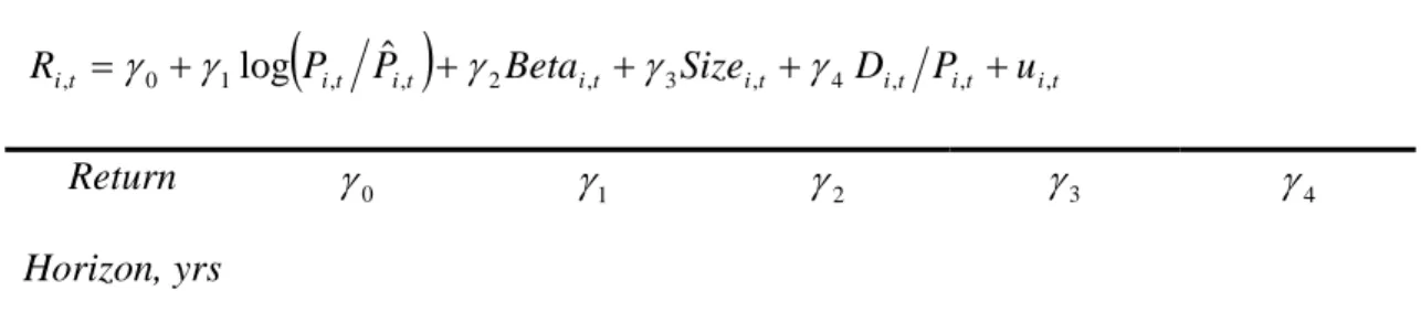
On our best estimate it is possible to earn substantial profits using this trading rule. We turn next to the question of whether these profits are statistically significant. We regress returns on the ration of market price to the theoretical stock price. We argued above that this ration should not be correlated with the risk of the stock providing the firm risk is constant over time. If this assumption is valid then a properly specified returns regression requires that we also include regressors which do explicitly capture risk. We use three variables to measure risk, Beta, size and dividend yield. Under the CAPM covariance with the market, i.e. Beta, measures risk. Fama and French (1992), and others, show that market capitalisation is important in explaining cross-section returns. Berk (1995) shows why size will serve as a risk measure. Finally , Ball (1978) argued that dividend yield should serve as a catch all measure of risk in an efficient market. Even if the researcher has not assumed the correct model of risk pricing then the variance of total returns due to risk will be proxied by the dividend yield, since the dividend yield is a component of the total return.9 This gives the specification of our cross-section regression, estimated at date t:
(
it it)
it it it it it t i P P Beta Size D P u R, =γ0 +γ1log , ˆ, +γ2 , +γ3 , +γ4 , , + , (3) 8Moreover, the average probability of a company which was in OV1 one year re-appearing in OV1 the following year was 53.8%. The average probability of a UN1 company re-appearing the following year was 43.5%. Mispricing is highly persistent, both for over and under-valued firms. However, the persistence of over valuation is rather greater than that of under valuation. This is consistent with the evidence in Table 2.
9
The only assumption required for this argument is that if dividends are paid on stock then the fraction of total returns which are delivered by dividends is not itself systematically related to risk.
The null hypothesis of efficient markets implies that γ1 =0: deviations of market price from the theoretical price reflect expected temporary deviations in the dividend growth rate from its long run average and are uncorrelated with subsequent returns.
Since firms are drawn from single economy we would expect a macro component to unexpected returns common to all firms at a single date, so ‘t’ statistic from the cross-section regression (3) will be biased because we would not expect cov
(
ui,uj)
≠0,. We follow Fama and Mcbeth (1973) (FM) proposed solution to this problem which recognises that the estimates of the coefficients themselves are not biased, despite the presence of cross-section dependence in the error term. Therefore regression (3) is estimated for t periods and the sample distribution of
j i≠
k
γˆ is constructed for each coefficient, k =0,...4. The sample standard deviation of the estimated coefficients provides an estimate of the standard error of the distribution of
k
γ . We then have the ‘t’ statistic
( )
k k k t γˆ =γˆ σˆγ for = 0,…4, where and k
∑
= − = T t kt k T 1 , 1 ˆ ˆ γ γ =(
−)
∑
T=(
−)
t kt k T k 1 2 , 2 2 ˆ ˆ 1 ˆ γ γσγ and T is the number of estimated
cross-section regressions. A disadvantage of this approach is that we cannot study long horizon returns, as FM estimation requires non-overlapping data. In order to run a reasonable number of independent cross-section regressions we only consider returns for horizons of up to three years. We retain the same start date, 1960. The cross-section regression is estimated each year 1960-91 for one year returns; every second year 1960-1990 for two year returns and every three years 1960-1989 for three year returns. This gave 15 two year horizon regression and 10 three year horizon regressions. We report the results in Table 3.
Table 3 shows that for return horizons of two and three years we can reject the implication of the efficient markets hypothesis that γ1 =0. The signs and ‘t’ statistics on the remaining variables are all largely in line with results obtained in previous research. The size variable is significant and of the expected sign in our sample. The dividend yield coefficient is of the expected sign for most periods. Although it is not statistically significant, we do not attach any importance to this in view of the few years available from which to calculate the ‘t’ statistic. For the same reason, the positive, but only marginally significant coefficient on Beta is unsurprising. The fact that we could run so few regressions to build up the sample distribution of the coefficients in the case of two and three year returns implies that our best test had low power to reject the null hypothesis. It is therefore the more striking that we were able to do so. It is interesting to compare the ‘t’ statistic on our mispricing variable with the evidence which our test delivers on the role of size. It is widely accepted that size is an important determinant of returns over this same time period, Fama and French (1992). However, the ‘t’ statistic on size in ours test is still smaller than that on the mispricing variable for both two and three year returns.
4. IS OUR CRITERION SIMPLY SELECTING RISKIER STOCKS?
The excess returns on the under priced portfolios appear to be large and statistically significant. However, it might yet be argued that the above assumption, that firms’ perceived relative risk at any time is the historic average up to that date in the sample, is invalid. In this case stocks which are of temporarily high risk will appear underpriced. One answer to this is that in the above regression we controlled for risk using the contemporaneously measured size and dividend yield and Beta measured
over the previous five years. Another perspective is provided by looking at the average value of size and Beta for the under and over-valued portfolios, and these statistics are reported in Table 4.
It can be seen in Table 4 that although the average value of Beta for the 5% most under-valued portfolio is larger than for the 5% most over-valued, the size of the difference is bot large enough to account for all the excess return. If the equity premium over the safe rate of interest is taken to be the historic average of approximately 8%, then the difference in Beta between UN1 and OV1 requires a yield difference of approximately 9% per annum over the first five years. Furthermore the average value of Beta for UN2 is less than for OV1, and yet on average for every horizon UN2 beats OV1.
The average company size in both of the under-valued portfolios is greater than in both of the over-valued portfolios. Since there is overwhelming evidence, Banz (1981), Fama and French (1992), that on average smaller firms deliver higher returns it is striking that UN1 and UN2 both beat OV1 and OV2 despite the fact that the latter are comprised on average of significantly smaller firms.
However many measures of risk we report it can still be argued that excess returns may be rationalised by some other model of risk. An alternative approach is to not focus on ex ante risk measures but to examine instead whether as a matter of fact the under priced shares were, when combined into portfolios, riskier ex post. That is, rather than comparing just the mean of the resulting returns distribution for under
priced / over priced portfolios, as in the previous section we compare the whole distributions. We report results on the distribution of five year returns in Table 5.
We examine whether a risk-averse individual would strictly prefer the distribution of returns from the under priced portfolio to the distribution of returns from the over priced portfolio. We use the criterion of second order stochastic dominance (SSD). A probability density function, , is said to exhibit SSD over a density if
, with strict inequality for some , where denote cumulative density functions associated with density functions and
f g
( )
( )
∫
y ≤∫
a y a G x dx dx x F ∀y y F,G f g respectively. If f exhibits SSD with respect to g, then f is preferred to g by all risk averters, see Rothschild and Stiglitz (1972).We find that the Decile of most under-valued shares exhibited second order stochastic dominance over the Decile portfolio of most over-valued shares. Indeed the under valued stocks only fail to exhibit first order stochastic dominance by a tiny margin. Table 5 reveals that for every start date the five year returns of the most under-valued Decile were greater than the five year returns on the most over-valued Decile, with the trivial exception of 1964 where the cumulative difference between the two was 0.3% over 5 years. To interpret the dominance of our under priced portfolios over five years as consistent with rational asset pricing one would have to argue that the excess return on the under priced stocks reflected a stronger positive covariance with shocks to aggregate wealth of a kind that was not observed in over thirty years.
Finally, consider the relative protection offered by the under and over priced portfolios to crashes. The largest annual fall in our sample, with average twelve
month returns of -29.7%, was in 1974. In all cases which overlap this period the most under valued portfolio 5 year returns still beat the most over valued portfolio. The under priced portfolio bought in December 1969 lost, by the end of 1974, 54.2% against a loss of 49.7% on the corresponding over priced portfolio.
We conclude that it seems hard to account for the profits delivered by the trading rule as equilibrium rewards to holding riskier stocks.
V Summary and Conclusions
We found support for the hypothesis that there is a component of forecastable stock returns which is driven by irrational swings in market sentiment. We employed a number of distinct approaches to the question of whether the returns forecastability we uncovered could be rationalised as an equilibrium reward to risk. Firstly, we worked with a benchmark price ratio which did not imply that risky shares would necessarily appear under priced, unlike those price scaled accounting variables which have previously been shown to forecast returns. Secondly we used a number of approaches to evaluate whether the portfolios of stocks which appear under priced were more risky. Each approach gave the same negative answer. This evidence suggests that one would have to have a very strong prior belief in efficient markets to argue that the stock picking rule we have used does not generate economic profits.
Our results provide a framework in which the evidence for negative serial correlation in long run returns reported by DeBondt and Thaler (1985) can be interpreted. Undervalued stocks must have delivered negative returns in the course of becoming
undervalued and hence the use of past returns will be a proxy for a direct measure of current mispricing. However, it is an imperfect proxy since we showed that excess returns which resulted from an unravelling of earlier mispricing were not correlated with subsequent returns.
An interesting extension of this work would be to try to find variables to explain the mispricing of equities as measured by Pˆi,t Pi,t
REFERENCES
Ball, R., (1978), Anomalies in Relationships Between Securities’ Yields and Yield-surrogates, Journal of Financial Economics, 6, 103-26.
Banz, R. W., (1981), The Relationship Between Return and Market Value of Common Stocks, Journal of Financial Economics, 9, 3-18.
Berk, J. B., (1995), A Critique of Size Related Anomalies, Review of Financial Studies, 8, 275-86.
Campbell J. Y. and R. J. Shiller, (1987), Co-integration and Tests of Present Value Models, Journal of Political Economy, 95, 1062-88.
Christie, W. G., (1990), Dividend Yield and Expected Returns: The Zero-Dividend Puzzle., Journal of Financial Economics, 28, 95-125.
DeBondt, W. F. M. and R. H. Thaler, (1985), Does the Stock Market Overreact? Journal of Finance, 40, 793-805.
Elton, E., M. Gruber and J. Rentzler, (1983), A Simple Examination of the Empirical Relationship Between Dividend Yields and Deviations from the CAPM, Journal of Banking and Finance, 25, 383-417.
Fama E. F. and J. D. MacBeth, (1973), Risk, Return and Equilibrium: Empirical Tests, Journal of Political Economy, 81, 607-636.
Fama E. F. and K. R. French, (1992), The Cross Section of Expected Stock Returns, Journal of Finance, 47, 427-65.
Lakonishok, J., A. Shleifer and R. Vishny, (1994), Contrarian Investment, Extrapolation and Risk, Journal of Finance, 49, 1541-1578.
Rothschild M., and J. E. Stiglitz, (1972), Increasing Risk II: Its Economic Consequences, Journal of Economic Theory, 3, 457-98.
Table 1. Average Cumulative Portfolio Returns Expressed as Percentage. Holding
Period, yrs
Full Sample FS
UN1 UN2 OV2 OV1
1 9.7 15.3 11.9 7.5 9.9 2 18.9 32.1 26.1 12.1 15.2 3 29.1 46.9 37.1 18.3 22.2 4 41.1 69.0 51.3 25.5 31.7 5 559 92.0 69.9 38.5 46.3 6 70.0 108.2 85.5 51.2 58.4 7 86.6 130.0 104.6 67.5 67.4 8 100.4 154.9 124.5 76.8 69.3 9 114.8 178.1 148.4 86.6 70.5 10 133.4 197.0 175.3 96.9 74.7
Table 2. Average Incremental Portfolio Returns Expressed as Percentage Holding
Period yrs
Full Sample FS
UN1 UN2 OV2 OV1
1 9.7 15.3 11.9 7.5 9.9 2 8.4 14.6 12.7 4.3 4.8 3 8.6 11.2 8.2 5.5 6.1 4 9.3 15.0 10.4 6.1 7.7 5 10.5 13.6 12.3 10.4 11.1 6 9.1 8.4 9.2 9.2 8.3
7 9.8 10.5 10.3 10.8 5.7
8 7.6 10.8 9.7 5.6 1.1
9 7.2 9.1 10.6 5.5 0.7
10 8.7 6.7 10.8 5.5 2.5
Table 3. Averaged Coefficients for Returns Regressions
(
it it)
it it it it it t i P P Beta Size D P u R, =γ0 +γ1log , ˆ, +γ2 , +γ3 , +γ4 , , + , Return Horizon, yrs 0 γ γ1 γ2 γ3 γ4 1 0.049 (1.76) -0.003 (-0.34) 0.059 (1.60) -0.016 (-2.25) 0.048 (0.21) 2 0.156 (2.74) -0.053 (-2.58) 0.038 (0.66) -0.030 (-1.99) -0.110 (-0.17) 3 0.226 (3.71) -0.106 (-2.39) 0.045 (0.94) -0.037 (-1.45) 0.623 (1.05)Table 4 Average Value of Beta and Company Size
Full Sample UN1 UN2 OV2 OV1
Beta 1.17 1.46 1.25 1.2 1.29
Table 5. Five Year Returns on Decile Portfolios Ranked by Pi,t Pˆi,t Start Date Most Under-valued Decile Most Over-valued Decile 1960 177.0 116.0 134.2 101.9 103.3 100.0 97.8 86.3 90.3 92.8 1961 51.9 59.9 59.1 40.0 38.3 35.1 37.0 37.3 54.0 32.3 1962 184.2 130.9 138.5 117.7 114.7 133.6 115.6 103.4 115.5 150.9 1963 171.2 151.4 116.6 86.6 107.0 133.9 153.9 133.2 163.2 154.6 1964 70.2 63.6 36.6 57.2 46.9 32.6 61.3 62.1 81.7 70.5 1965 26.2 15.9 13.5 16.4 34.9 19.4 54.1 5.6 7.9 0.4 1966 86.8 47.8 50.0 44.8 61.2 67.4 47.3 28.0 64.1 28.9 1967 14.1 32.2 23.8 27.0 20.7 18.7 8.4 15.0 5.9 -21.7 1968 -24.3 -15.9 -21.6 -15.5 -17.1 -37.8 -16.3 -32.6 -39.2 -51.4 1969 -34.2 -34.7 -33.7 -31.4 -34.7 -33.7 -24.0 -36.5 -56.1 -49.7 1970 -6.8 -11.4 -17.8 -7.9 -19.3 -16.4 -12.6 -11.7 -14.6 -8.3 1971 16.5 0.6 10.1 11.9 5.2 -0.8 -16.3 3.2 2.4 -16.0 1972 0.1 -5.3 -4.3 -9.1 -1.4 -8.9 3.4 -22.2 -16.5 -10.7 1973 71.4 48.6 40.8 37.7 34.0 42.4 17.9 -10.2 -13.7 -14.7 1974 169.8 146.4 142.4 103.1 85.0 84.5 97.8 84.4 85.6 74.1 1975 98.8 71.5 77.8 67.5 82.1 77.6 47.0 44.1 52.2 62.1 1976 26.1 22.2 9.5 6.2 28.0 16.3 16.2 29.9 16.7 23.6 1977 73.1 34.5 23.7 62.6 41.9 57.1 27.3 23.6 69.0 57.1
1978 120.0 56.9 87.1 105.0 64.0 91.9 101.4 91.4 88.8 97.8 1979 107.6 68.0 70.1 71.0 35.8 73.1 51.3 53.9 56.5 37.5 1980 156.8 144.7 148.6 101.5 88.3 89.8 96.0 47.3 34.2 54.9 1981 208.8 193.5 179.4 186.7 142.0 126.9 90.0 127.8 102.3 99.8 1982 117.3 148.6 161.7 155.6 148.9 125.7 101.9 123.5 111.9 114.2