B
Evaluation of forecasts by accuracy and spread in the MiKlip
decadal climate prediction system
Christopher Kadow1∗, Sebastian Illing1, Oliver Kunst1,2, Henning W. Rust1, Holger Pohlmann3, Wolfgang A. Müller3and Ulrich Cubasch1
1Institute of Meteorology, Freie Universität Berlin, Berlin, Germany 2Zuse Institute Berlin (ZIB), Berlin, Germany
3Max-Planck-Institute for Meteorology, Hamburg, Germany
(Manuscript received July 31, 2014; in revised form April 21, 2015; accepted April 22, 2015) Abstract
We present the evaluation of temperature and precipitation forecasts obtained with the MiKlip decadal climate prediction system. These decadal hindcast experiments are verified with respect to the accuracy of the ensemble mean and the ensemble spread as a representative for the forecast uncertainty. The skill assessment follows the verification framework already used by the decadal prediction community, but enhanced with additional evaluation techniques like the logarithmic ensemble spread score. The core of the MiKlip system is the coupled Max Planck Institute Earth System Model. An ensemble of 10 members is initialized annually with ocean and atmosphere reanalyses of the European Centre for Medium-Range Weather Forecasts. For assessing the effect of the initialization, we compare these predictions to uninitialized climate projections with the same model system. Initialization improves the accuracy of temperature and precipitation forecasts in year 1, particularly in the Pacific region. The ensemble spread well represents the forecast uncertainty in lead year 1, except in the tropics. This estimate of prediction skill creates confidence in the respective 2014 forecasts, which depict less precipitation in the tropics and a warming almost everywhere. However, large cooling patterns appear in the Northern Hemisphere, the Pacific South America and the Southern Ocean. Forecasts for 2015 to 2022 show even warmer temperatures than for 2014, especially over the continents. The evaluation of lead years 2 to 9 for temperature shows skill globally with the exception of the eastern Pacific. The ensemble spread can again be used as an estimate of the forecast uncertainty in many regions: It improves over the tropics compared to lead year 1. Due to a reduction of the conditional bias, the decadal predictions of the initialized system gain skill in the accuracy compared to the uninitialized simulations in the lead years 2 to 9. Furthermore, we show that increasing the ensemble size improves the MiKlip decadal climate prediction system for all lead years.
Keywords: Decadal Prediction, Climate, Forecasts, Evaluation, Metrics
1
Introduction
Decadal climate prediction research gains progressively more attention in climate science as well as in society, industry and economy. The research aims to close the gap between short term forecasts and long term projec-tions. Numerical weather predictions focus on an initial value problem in the beginning of a forecast. On the other hand, climate projections as a boundary condition problem examine the long-term development (Meehl et al., 2009;Mehta et al., 2011). In order to accommo-date the demand for reliable informations on near-term climate variability on the crucial timescales of a year up to a decade, different national and international initia-tives have been launched. The Coupled Model Intercom-parison Project Phase 5 (CMIP5, Taylor et al., 2012) offers a platform to approach decadal predictions on a common basis via hindcast experiments in the ‘observa-tion’ period from 1960 to 2010.
∗Corresponding author: Christopher Kadow, Institute of Meteorology, Freie
Universität Berlin, Carl-Heinrich-Becker-Weg 6–10, 12165 Berlin, Germany, e-mail: [email protected]
The ‘Mittelfristige Klimaprognosen’ (MiKlip) pro-ject, funded by the Federal Ministry of Education and Research in Germany (BMBF), is based on CMIP5 and currently develops a decadal forecast system us-ing the Max Planck Institute Earth System Model (MPI-ESM). With the improvements made through initializa-tion techniques using ocean and atmosphere reanalyses in a coupled initialization(Pohlmann et al., 2013), the MiKlip model version outperforms the CMIP5 comple-ment(Müller et al., 2012), especially in the tropics.
In this study we present the forecasts and the skill assessment of the MiKlip decadal climate predic-tion system following the verificapredic-tion framework for interannual-to-decadal prediction experiments recom-mended byGoddard et al. (2013). For this purpose, we employ the decadal evaluation tool ‘MurCSS’ (Illing et al., 2014) as part of the MiKlip Central Evaluation System. We point out the importance of a detailed eval-uation by combining initialized decadal climate predic-tions with their prediction skill using the MiKlip sys-tem. In Section2we present the statistical methods used to evaluate the accuracy and the spread of the
ensem-© 2015 The authors DOI 10.1127/metz/2015/0639 Gebrüder Borntraeger Science Publishers, Stuttgart,www.borntraeger-cramer.com
ble hindcast experiment. We present decadal forecasts and their prediction skill for near surface air temperature and precipitation for lead year 1 and lead years 2 to 9, as well as the improvement due to increased ensemble size in Section3. In Section4, we discuss the combina-tion of prediccombina-tions and the prediccombina-tion skill of the MiKlip system.
2
Data and methods
The MiKlip decadal forecasts and hindcasts (Base-line1, see also Pohlmann et al., 2013) used in this study were conducted with the earth system model from the Max-Planck-Institute in the low resolution ver-sion (MPI-ESM-LR). It is a coupled atmosphere-ocean system triggered by two different initialization
tech-niques. The ocean component MPI-OM (Jungclaus
et al., 2013)with the resolution of 1.5 °/L40 was initial-ized with temperature and salinity anomaly fields from the European Centre for Medium-Range Weather Fore-casts (ECMWF) ocean reanalysis system 4 (ORAS4 –
Balmaseda et al., 2013). The atmospheric component ECHAM6(Stevens et al., 2013) with the resolution of T63L47 was obtained by a full-field initialization with ECMWF atmosphere reanalyses, including fields of temperature, vorticity, divergence, and surface pressure (ERA40 in 1960–1989 and ERA-Interim in 1990–2013,
Uppala et al. (2005)andDee et al. (2011)respectively). The simulations were started annually for the period 1961 to 2013, each initialization simulating a decade and consisting of 10 ensemble members.
Uninitialized runs with the same model configura-tion and in the same time period serve as references (Goddard et al., 2013; Matei et al., 2012), disclosing the effect of the initialization and its potential gain of skill. The uninitialized simulations equate to the ‘his-torical’ experiment performed during CMIP5 using ob-served external forcings. Due to the fact that the ‘his-torical’ experiment ends in 2005, the reference run was extended by the CMIP5 ‘rcp45’ experiment consisting of the projected RCP4.5 scenario(Taylor et al., 2012). A 10 member experiment of uninitialized runs was con-ducted to have an equivalent ensemble size to the initial-ized runs.
We compare near surface air temperature to the Had-CRUT3v(Brohan et al., 2006)dataset from the Hadley Centre and Climatic Research Unit for the period 1961 to 2012. This commonly used anomaly data set is cho-sen to maintain the comparability to other decadal pre-diction studies(Pohlmann et al., 2013;Goddard et al.,
2013;Matei et al., 2012). To enable a global compar-ison of precipitation with observation over land and ocean, a shorter time period was selected, focussing on the era of satellite data. The Global Precipitation Cli-matology Project Satellite-Gauge (GPCP-SG) dataset (Adler et al., 2003) was used for the period from 1979 to 2012. However, for full comparablity with the decadal prediction community and the evaluation over the longer
timescale, we also present the evaluation of precipi-tation with the Global Precipiprecipi-tation Climatology Cen-tre (GPCC) Full Data Reanalysis Version 6 dataset (Schneider et al., 2011;Becker et al., 2013)over land in the supplementary material of this publication. For both evaluated variables, anomalies are considered for comparison with the model data to ensure that no gen-eral bias is influencing the results like differences in the height of model and observation.
The anomaly real-time forecasts for temperature and precipitation are available for the year 2014 and the time period of the years 2015 to 2022. The reference period is 1981 to 2010. The uninitialized simulations are used as reference datasets for the anomaly calculations.
The following skill assessment – based on the decadal climate prediction verification framework
(God-dard et al., 2013) – includes spatial averaging on a 5×5 degree grid, temporal aggregation and lead-time dependent bias adjustment in a cross validated manner (ICPO, 2011). The lead year 1 hindcast continues the observed initial conditions in the first prediction year. For the lead years 2 to 9, the representation of the decadal-scale climate predictions excludes the skill of lead year 1. Significance of the verification scores was estimated using a non-parametric bootstrap approach (Wilks, 2005;Mason and Mimmack, 1992)taking au-tocorrelation into account(Goddard et al., 2013). First, we investigate the gain of accuracy in the ensemble mean due to the initial conditions compared to unini-tialized climate change projections. In a second step, we analyze whether the ensemble spread is an appropriate representation of the forecast uncertainty on average.
2.1 Accuracy of the ensemble mean
The mean squared error skill score (MSESS) compares the accuracy of two predictions (Murphy, 1988)of the past, so called hindcasts. The initialized hindcasts Hi j
consist of their ensemble members i = 1, . . . ,m and
the start times j = 1, . . . ,n. The mean squared error
(MSE) between the hindcast ensemble mean Hjand the
observations Oj over j = 1, . . . ,n start times can be
expressed as MSEH = 1 n n j=1 (Hj−Oj)2. (2.1)
Compared to some reference prediction, such as the climatological forecast MSEO¯ = 1nnj=1( ¯O−Oj)2, the
skill can be determined by the
MSESS(H,O¯,O)=1−MSEH MSEO¯
. (2.2)
Applying the Murphy-Epstein decomposition and using anomalies, the MSESS for the climatological forecast
can be written as: MSESS(H,O¯,O)=r2HO− rHO− sH sO 2 (2.3)
with rHO being the sample correlation coefficient
be-tween the hindcasts and the observations, and the sample variance of the hindcasts s2Hand observations s2O
(Mur-phy, 1988;Murphy and Epstein, 1989). This decom-position allows to differentiate between the correlation coefficient and the conditional prediction bias (second term on the right hand side of Eq.2.3). When compar-ing the initialized hindcasts H with the uninitialized ref-erence R, the MSESS can be written as
MSESS(H,R,O)= MSESSH−MSESSR
1−MSESSR
(2.4) to assess the change of skill from the uninitialized to the initialized prediction system.
The MSESS represents the improvement in the ac-curacy of the hindcasts H over the climatology ¯O or a
reference forecast R with respect to the observations O, where−∞ <MSESS≤ 1. A positive value suggests an improved accuracy of the hindcast ensemble mean com-pared to the reference, and a negative value indicates the opposite.
The correlation coefficient −1 ≤ r ≤ 1 as the po-tential skill of a prediction system represents the linear relationship between a hindcast and the observation. For assessing the change in the correlation coefficient of the hindcast against a reference prediction, the difference of
rHO and rROis presented, with values ranging from −2
to 2.
The conditional bias−∞< rHO− ssHO < ∞is the
dif-ference of the correlation and the ratio of standard devi-ation from a prediction and observdevi-ation – it is zero at its best. The gain of the conditional bias against a reference prediction is calculated by subtracting the absolute val-ues|rRO − ssOR| − |rHO− ssHO|. Positive values represent a
decrease of bias or, in the sense of the MSESS, a gain of skill and vice versa.
2.2 Ensemble spread as forecast uncertainty
The spread of an ensemble forecast (ensemble variance) is meant to be an estimate of the forecast uncertainty due to uncertainty in the initial conditions. If the mean squared deviation of the observations from the ensemble mean (MSE) corresponds to the ensemble variance, the latter is a good estimate of the forecast uncertainty. Is the ensemble variance smaller than the MSE the ensem-ble is said to be under-dispersive (overconfident); an en-semble variance larger than the MSE indicates an over-dispersive (underconfident) ensemble. This answers the question, if the ensemble spread can be used as refer-ence for the forecast uncertainty. Following Goddard
et al. (2013), the ensemble spread is compared to the
forecast uncertainty using a particular version of the continuous ranked probability skill score (CRPSS). The CRPSS is based on the continuous ranked probability score(Matheson and Winkler, 1976)
CRPS(Hi j,Oj)=
∞
−∞(FHj(y)− H(y−Oj))
2dy, (2.5)
which integrates the squared difference between the probability distribution FHjof the ensemble forecast and
the observation for a given instance j = 1, . . . ,n in
probability space over the predictand y. The Heaviside functionH(y−Oj) is the associate cumulative
distribu-tion funcdistribu-tion for the single observadistribu-tion. Gneiting and Raftery (2007)suggested to use a normal distribution with mean Hj and variance σ2H for the forecast
proba-bility density function FHj = N(Hj, σ
2
Hj). The CRPS
can be expressed with the standard normal probability density and cumulative distribution functionϕandφ, re-spectively CRPS(N(Hj, σ2Hj),Oj)= σHj 1 √π−2ϕ Oj−Hj σHj −Ojσ−Hj Hj 2φ Oj−Hj σHj −1 . (2.6) To quantify the ensemble spread against the standard error, we use the average ensemble spread
σ2 ˆ H = 1 n n j=1 1 m−1 m i=1 ( ˆHi j−Hˆj)2 (2.7)
with the ensemble members ˆHi j and the ensemble mean
ˆ
Hj corrected for mean and conditional bias. The
refer-ence prediction has the same mean, but its variance is replaced by the MSE
σ2 R = 1 n−2 n j=1 ( ˆHj−Oj)2. (2.8)
Using these hindcast and reference distributions in the continuous ranked probability skill score for the assess-ment of the ensemble spread, the resulting CRPSSES reads CRPSSES =1− jCRPSH(N( ˆHj, σ2Hˆ),Oj) jCRPSR(N( ˆHj, σ2R),Oj) . (2.9)
The reference CRPSR using the MSE represents the
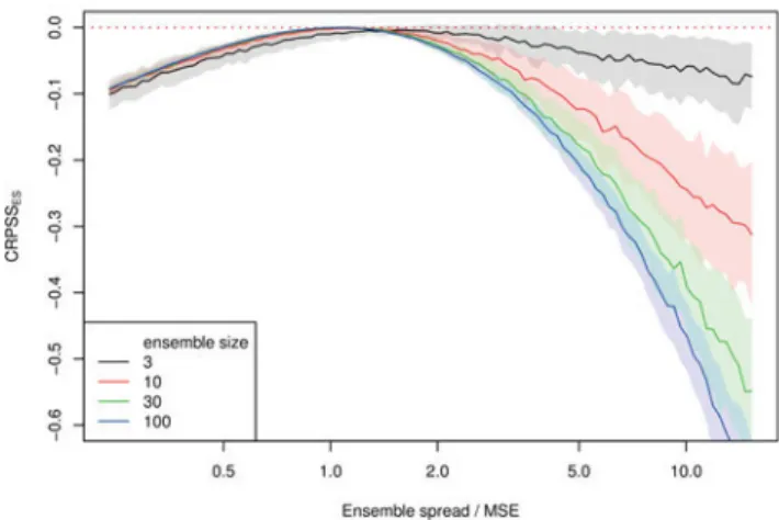
forecast uncertainty and thus defines the desired value for the CRPSH, therefore CRPSSES ≤ 0. The optimum
Figure 1: The CRPSSESas function of the ratio between ensemble
spread (σ2 ˆ
H) and MSE (σ
2
R) for different ensemble sizes. When the
given ratio is one, the CRPSSESreaches its maximum value of zero.
CRPSSES = 0 is attained for σ2Hˆ = σR2, and σ2Hˆ σ2R leads to a negative CRPSSES. The respective simulation study with varying ensemble size is utilized in Figure1. This behavior does not allow to determine whether the ensemble spread is over- or underestimating the forecast uncertainty (MSE). To add this missing information, we consider the spread score (see Palmer et al., 2006;
Keller et al., 2008), with a log-transform to obtain the logarithmic ensemble spread score
LESS=ln ⎛ ⎜⎜⎜⎜⎜ ⎜⎜⎜⎝σ 2 ˆ H σ2 R ⎞ ⎟⎟⎟⎟⎟ ⎟⎟⎟⎠. (2.10)
The LESS shows negative (positive) values for under-dispersive (over-under-dispersive) forecasts. A meaningful combination of the CRPSSES and the LESS depicts the skill and the sign of dispersion. This addresses the ques-tion whether the ensemble spread is an adequate rep-resentation of the forecast uncertainty on average posed byGoddard et al. (2013). In this study, we define a skill score based on the LESS to compare model development stages. Different sized ensembles of the model system can be evaluated with respect to spread development.
LESSS=1− LESS
2 pred
LESS2ref ∈(−∞,1] (2.11)
The LESSS answers the question if the prediction sys-tem improves this ratio between the average ensemble spread and the mean squared error compared to the ref-erence prediction.
3
Results
3.1 Forecasts and skill assessment of
temperature
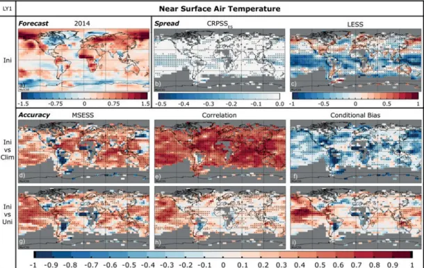
In general, the anomaly forecast of near surface air temperature for the year 2014 with the MiKlip system shows rather warming than cooling signals in the dif-ferent regions of the world (Figure 2a). However, there are regions with strong negative and positive signals. The North-East Pacific, the western part of North Amer-ica including Alaska, Central and Southern AfrAmer-ica as well as Russia show distinct hot spots with anomalies over 1.5 K. There are cooling patterns as well, mainly over the north-eastern North-America, India and south-ern China, the Antarctic Circumpolar Current and the northern North Atlantic. The forecast for the eastern Pa-cific points to a cooling in the ENSO region and positive anomalies in the surrounding. Over Europe, the forecast shows a warming of around 0.75 K. The climate forecast for the years 2015 to 2022 predicts a clear warming sig-nal on the Northern Hemisphere from 60 ° N northwards with values over 1.5 K, beside the cooling spot in the northern North-Atlantic (Figure3a). The forecast shows also a cooling area in the Pacific-Antarctic Basin, e.g. over the Amundsen Sea. All continents show a warming signal of around 1 K, as do the equatorial eastern Pacific, the eastern Atlantic, and the western Indian Ocean.
The analysis of the near surface air temperature in lead year 1 indicates an improvement from the unini-tialized projections to the iniunini-tialized hindcasts (Fig-ure 2g,h,i). Combining the effect of increased correla-tion and reduced condicorrela-tional bias, the MSESS exhibits significant positive values over the ocean, most likely due to the ocean initialization. The North Pacific in par-ticular benefits from the initialization (Figure 2g). The North Atlantic provides a contrast: while there is at least some improvement in correlation compared to the unini-tialized runs (Figure2h), it is accompanied by a decrease in the conditional bias (Figure2i). The initialized hind-cast experiments (Figure 2) of lead year 1 add confi-dence to the forecast of surface temperature in Figure2a. For lead years 2 to 9 (see Figure 3), the initialized and uninitialized experiments perform similarly. Due to catching the long-term trend of the climate system, the correlation coefficients for surface temperature are sig-nificantly high. Apart from the ENSO-related tropical Pacific, this is comparable toGoddard et al. (2013)and
Müller et al. (2012). Little correlation is lost almost over the whole globe in the initialized runs compared to the historical runs (Figure3h). However, small areas of positive gain in correlation can be found in the North At-lantic (Figure 3h). The conditional bias (Figure3f) im-proved in the initialized runs, leading to an overall posi-tive skill (Figure3i). The MSESS in the initialized runs against uninitialized hindcast for the surface tempera-ture increases significantly in the tropics (Figure3g). It decreases over areas such as northern Asia and suffers
Figure 2: Anomaly forecast of the MiKlip decadal prediction system for near surface air temperature in Kelvin for the year 2014 (a).
Anomalies are calculated relative to the years 1981 to 2010 from the uninitialized (historical and rcp45) simulations and interpolated on the 5×5 ° grid for skill assessment. The evaluation of the ensemble spread is to the right of the forecast with the continuous ranked probability skill score of the ensemble spread vs the reference error (CRPSSES in b) and the logarithmic ensemble spread score (LESS in c). The
ensemble mean hindcast skill is shown in the middle and bottom row – mean squared error skill score (MSESS – left column) and its decomposition in correlation (middle column) and conditional bias (right column) of near surface air temperature averaged over the first prediction year against observation from HadCRUT3v over the period 1961–2012. It shows the skill of the initialized decadal experiments against a climatological forecast (middle row) including the MSESS (d), correlation (e) and the conditional bias (f). The lower row uses the uninitialized simulations (historical, extended with rcp45 to year 2012) as the reference prediction in the MSESS (g), the correlation differences (h) and depicting the change in magnitude of the conditional bias (i). Colorbars in the accuracy section are scaled to−1 to 1. Crosses denote values significantly different from zero exceeding at a 5 % level applying 1000 bootstraps. Gray areas mark missing values with less than 90 % data consistency in the observation.
from an increased conditional bias and negative correla-tion.
The CRPSSESin Figure2b,3b shows that the ensem-ble spread can represent forecast uncertainty in various regions. This is not the case in the central Pacific for lead year 1 (Figure2b). The LESS in Figure2c reveals that the spread is too small in the tropics and the South-ern Hemisphere; this improves slightly for years 2 to 9 (Figure 3c). Variabilities around the North Atlantic as well as the North Pacific in lead year 1 (Figure2c) show patterns with over- and under-dispersive spreads next to each other. The ensemble is over-dispersive for North America, the North Atlantic, Europe as well as around the Kuroshio, which means the ensemble spread is too large compared to the reference error (Figure2c,3c).
The model system used in this study also participates in a multi-model comparison project as accomplished by Smith et al. (2013). However, a different initializa-tion strategy is applied, when comparing the real-time forecasts. The anomaly initialization in the ocean was conducted through a NCEP forced assimilation run, so called MiKlip Baseline0 simulation (see Matei et al., 2012;Müller et al., 2012). The MiKlip system as an-alyzed in this study (Baseline1) is closer to the multi-model average as shown in Smith et al. (2013) than Baseline0 (not shown). In general a more uniform warm-ing (less regions with coolwarm-ing) is predicted with Base-line1 compared to Baseline0 on the longer timescales beyond lead year 1.
3.2 Forecasts and skill assessment of
precipitation
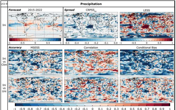
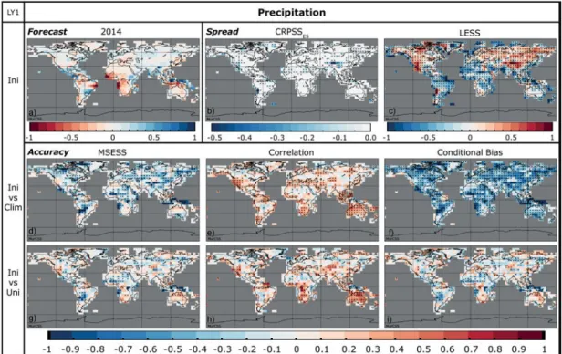
The prediction of precipitation is more challenging, and consequently results are more dispersive than for tem-perature. The forecasts feature strong anomalies in the tropics and over the oceans (Figure4a,5a). The anomaly forecast in Figure4a shows an increase in precipitation for the year 2014 in the northern West Pacific, East At-lantic and Indian Ocean. Precipitation is decreasing in the southern equatorial Pacific and Atlantic. The fore-casts over Africa and northern South America predict an overall drying, while Central America and India show a wetter signal. For the next 2 to 9 years (2015–2022) precipitation rates decrease over the northern equatorial Atlantic as well as south of the equator in the Indian Ocean and increase in the tropical Pacific. The latter shows El Niño like structures (Figure5a). In general, the continents in the northern hemisphere show an increase, whereas the southern continents including Africa rather indicate a decrease.
The evaluation of lead year 1 shows a significant gain in correlation for the initialized over the uninitial-ized experiment (Figure 4h). Significant positive corre-lation between the decadal hindcasts and the observa-tions from GPCP-SG (Figure 4e) is present mainly in the tropical Pacific, but can also be detected in the equa-torial Atlantic and the Indian ocean. Conditional biases
for initialized (Figure 4f) and uninitialized (Figure 4i) simulations are large and negative over the whole globe compared to GPCP-SG. In the tropics in particular, the model has difficulties to reproduce precipitation vari-ability. For the initialized run the performance is worse compared to the climatological forecast. However, the combined MSESS still shows some skill (Figure4d,g), which can be traced back to the strong improved corre-lation compared to the uninitialized simucorre-lations.
The various skill scores (Figure 5) become noisy for the lead years 2 to 9. However, we present these results as well – for consistency and comparability with other international studies(Goddard et al., 2013;
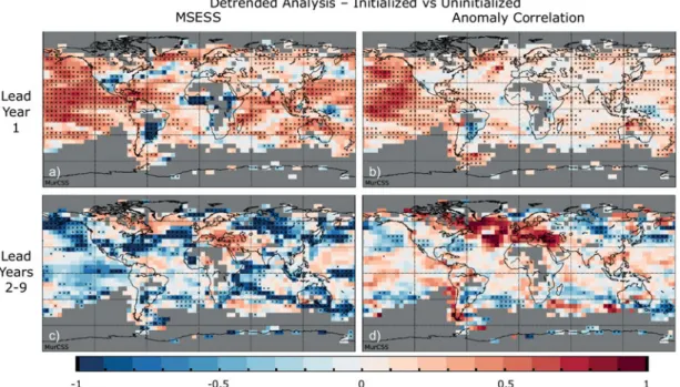
Smith et al., 2013). Some continental areas like Eu-rope, the Middle East and North-East Asia, as well as the Indian Ocean, show some positive correlation in the decadal hindcasts compared to the climatological fore-cast (Figure 5e). The decadal hindcasts improve over Europe when compared to the uninitialized simulations (Figure 5h). This comes along with an improved tem-perature and therefore energy budget over Europe when compared to the uninitialized hindcast for the lead years 2 to 9. This gets more obvious, when the initialized system clearly outperforms the uninitialized system in the detrended temperature analysis of the MSESS and correlation in the leadyears 2 to 9 (FigureS3). This is because annual precipitation is not that trend related (Kumar et al., 2013), especially in Europe (Cubasch and Kadow, 2011) and the North Atlantic is shown to be the source of skill over Europe (Ghosh et al., sub-mitted). But, due to the loss of correlation for precipi-tation in most of the other regions by contrast with the uninitialized runs and the negative conditional bias in the North Atlantic, as well as the same difficulties as ex-perienced for lead year 1 at the equatorial regions in the conditional bias (Figure 5f,i), the MSESS comparison from initialization runs versus uninitialized simulations (Figure5d,g) shows almost no skill for precipitation.
For lead year 1 the ensemble spread is an adequate estimate for the forecast uncertainty for most regions (Figure4b). This is no longer valid for lead years 2 to 9 (Figure 5b), with only some small areas left over the ocean with the spread being close to the reference error. The CRPSSEShighlights the areas in the tropical Pacific and Atlantic showing no skill. The LESS demonstrates the over-dispersion (Figure4c,5c) in these regions. Here, the precipitation rates suffer from positive temperature biases in the ocean in these areas (not shown), which leads to more convective activity and variability. Fur-thermore, the LESS reveals that areas of small and large ensemble spreads are next to each other in the central Pacific and Atlantic. This points to problems in the cor-rect representation of small scale processes on these time scales in the spread of the ensemble. Variabilities in convective and large scale precipitation processes in climate models are difficult to represent. The standard error of satellite instruments is also relatively high in re-gions with little precipitation, especially in the first years of the GPCP-SG dataset(Adler et al., 2003). The short
Figure 4: As in Figure2but for precipitation in mm/day and using the observation from GPCP-SG over the period 1979–2012 for skill assessment.
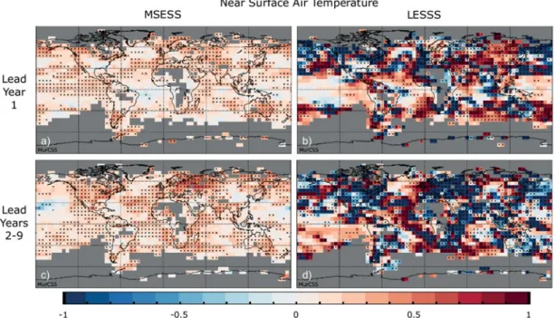
Figure 6: Comparison of the hindcast skill of different sized ensemble model versions (10 member vs 3 member). MSESS and LESSS for
near surface air temperature over the period 1961–2012 against HadCRUT3v for the lead year 1 (upper row) and lead years 2 to 9 (lower row). The MSESS shows the improvement made in the hindcast ensemble mean prediction and the LESSS exhibit the improvement in the ensemble spread as an adequate representation of the forecast uncertainty. Crosses denote values significantly different from zero exceeding at a 5 % level applying 1000 bootstraps. Gray areas mark missing values with with less than 90 % data consistency in the observation.
observational period of the satellite observations is prob-lematic too, when analyzing the lead years 2 to 9.
3.3 Ensemble Size
The CMIP5(Taylor et al., 2012)decadal experimental design with initializations every 5 years led to an un-reliable skill assessment (Goddard et al., 2013). Since then, most of the prediction systems are initialized an-nually. The small ensemble size of these experiments is another known issue, particularly for comparing differ-ent prediction systems(Smith et al., 2013).Pohlmann
et al. (2013) analyze only 3 ensemble members of the MiKlip system in order to have a clean comparison with the results of the 3 available members in the CMIP5 sys-tem.Kruschke et al. (2014)use a bias corrected RPSS to compensate for different ensemble sizes. A compre-hensive study on the effect of the ensemble size on decadal prediction is given in Sienz et al. (submitted). To fill the gap between the MiKlip system analyzed in
Pohlmann et al. (2013) and the results shown in this study, we present the change of skill for lead years 1 and 2 to 9 by increasing the ensemble size from 3 to 10 ensemble members.
The MSESS in Figure 6 shows a significant gain of prediction skill for surface temperature. Besides the Central Atlantic, the temperature prediction skill for lead year 1 increases for the whole globe – not sig-nificant everywhere (Figure 6a). But on the long run,
the forecast for the Central Atlantic benefits from the larger ensemble for lead years 2 to 9 (Figure 6c). The LESSS for temperature shown in Figures 6b) and 6d) improves in the tropics where the CRPSSESreveals sig-nificant negative skill (Figure2b,3b) and the LESS (Fig-ure 2c,3c) depicts an under-dispersion. Therefore, the decreasing under-dispersion due to the increased ensem-ble size leads to a slightly better representation of the uncertainty by the ensemble spread. Precipitation shows an improvement in the MSESS in lead years 1 and 2 to 9 (not shown). The LESSS improves only in local areas in the development of the ensemble spread as an adequate forecast uncertainty in the comparison of the 10 to the 3 ensemble member system for precipitation (not shown).
4
Discussion and conclusions
Combining forecasts and detailed evaluation for the MiKlip system for near surface air temperature and pre-cipitation provides a comprehensive assessment of the decadal climate predictions. With a strong impact in lead year 1, initialization techniques improve the pre-diction system in comparison to an uninitialized sys-tem. Both atmospheric parameters benefit from an ini-tialization with an oceanic reanalysis. Mainly the Pa-cific region temperature forecast improves, which causes an improved convection, triggering precipitation fluxes.
The equatorial regions suffer from an under-dispersive ensemble in temperature and an over-dispersion of pre-cipitation in regions of western South America over the Pacific and western Central Africa over the Atlantic. Both variables exhibit a large negative conditional bias in lead year 1. The largest temperature anomalies for year 2014 are forecasted in areas where the performance of the model system is less satisfying, e.g. a warming of 3 Kelvin in West Africa or a cooling of 2 Kelvin in a small region in the North Atlantic. Regions with few data for validation like the southern Pacific can not be reliably evaluated using observational reconstructions.
As the initialized system drifts towards the same state as the uninitialized model, the lead years 2 to 9 produce similarly performances for the initialized and uninitialized experiments. The improvement of the ini-tialized prediction system on these timescales stems from the decreased conditional bias in combination with an increased ensemble size, at least for temperature. The conditional bias exists, when a climate model e.g. over-responds to increasing greenhouse gases
(God-dard et al., 2013). This can result in an overestimation of temperature anomalies. In this respect, the initialized MiKlip prediction system performs better in the MSESS than the uninitialized due to matching the climate trend much better. But it is difficult to differentiate between a model drift of the initialized system towards a warmer state of the uninitialized system and a possible predicted warming after the hiatus(Meehl et al., 2011;Kosaka
and Xie, 2013). Analyzing a decadal prediction system being between an initial and boundary condition prob-lem leads to several factors for potential skill. The cor-rect initial condition in the beginning of the forecast improves the forecast on the seasonal to the interan-nual timescale. The memory of the ocean plays a big role on interannual to decadal timescale, when running a coupled model. But the trend due to increased green-house gases has even more influence on the long-term development. Analyzing the time range of 2 to 9 years mixes these potentials of skill and the uninitialized sys-tem improves on the long run. Therefore the uninitial-ized can outperform the initialuninitial-ized system in correla-tion like shown in this study. But, filtering the trend in the temperature hindcasts and observations showed that the initialized system beats the uninitialized simulations in terms of correlation on these timescales. However, the long-term temperature trend belongs to the 2 to 9 year forecast. This cannot be adjusted, when presenting decadal predictions.
The comparison of the 10 ensemble member sys-tem against the 3 ensemble member syssys-tem (used in
Pohlmann et al., 2013), shows clear improvements in the MSESS over the whole globe. Even for regions of overestimated precipitation, the forecasts improved for lead years 2 to 9. The analysis of the LESSS also shows a slight improvement in ensemble spread in the trop-ics, comparing two different ensemble sizes. In most of the regions the ensemble spread is an adequate rep-resentation for the uncertainty of this system and it is
much closer to the reference error (MSE) than for other decadal prediction systems(Goddard et al., 2013).
Including the LESS and the LESSS to the set of skill assessment for decadal prediction allows to dis-tinguish between an over- or under-dispersive ensem-ble and detect improvements made when aiming at larger ensemble sizes (Sienz et al., submitted). The LESSS could also be used to evaluate different ensem-ble generation methods of the same model system to as-sess their possible improvement. After the development stages and accomplished improvements(Müller et al., 2012; Pohlmann et al., 2013; Kruschke et al., 2014;
Stolzenberger et al., submitted;Spangehl et al.,
sub-mitted), the next step in the ongoing MiKlip project is to switch from the anomaly initialization in the ocean with ORAS4 to full-field multi-reanalysis initialization with ORAS4 and GECCO2 (Köhl, 2014). A first study on these combined predictions is given byKruschke et al.
(submitted). The coming 30 member prediction system will allow a more robust assessment. It will be possi-ble to involve other scores to this combined prediction system, e.g. the error spread score(Christensen et al., 2015), which needs ensemble sizes larger than available in this study.
The decadal skill assessment used in this study is an operational part of the central evaluation in MiKlip. It is available to the climate science community (Illing et al., 2014) and is planned to be deployed in the next stages of the MiKlip project development.
Acknowledgments
We acknowledge funding from the Federal Ministry of Education and Research in Germany (BMBF) through the research programme MiKlip1, projects IN-TEGRATION (FKZ: 01LP1160A), ENSDIVAL (FKZ: 01LP1104A), and FLEXFORDEC (FKZ: 01LP1144A). We have used observational data provided by the Hadley Centre2, Global Precipitation Climatology Project3, Global Precipitation Climatology Centre4 at Deutscher
Wetterdienst and reanalyses from the ECMWF5. The climate simulations were performed at the German Climate Computing Centre (DKRZ6). The skill as-sessment is part of the Central Evaluation System7 of MiKlip. The authors thank Mareike Schuster,
Tim Kruschke, Madlen Fischer and Martina Baltkalne whose comments helped to improve this
pa-per. 1http://www.fona-miklip.de/en 2http://www.metoffice.gov.uk/hadobs 3http://www.gewex.org/gpcpdata.htm 4http://gpcc.dwd.de/ 5http://www.ecmwf.int 6https://www.dkrz.de 7https://www-miklip.dkrz.de
Appendix
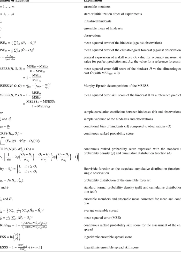
Table 1: Overview table of used variable names and equations.
Variable or Equation Explanation
i=1, . . . ,m ensemble members
j=1, . . . ,n start or initialization times of experiments
Hi j initialized hindcasts
Hj ensemble mean of hindcasts
Oj observations
MSEH=1n
n
j=1(Hj−Oj)2 mean squared error of the hindcast (against observation)
MSEO¯= 1n
n
j=1( ¯O−Oj)2 mean squared error of the climatological forecast (against observation)
ref=
A−Aref
Aperf−Aref general expression of a skill score (A value for accuracy measure, Aperfthe
value for perfect prediction and Arefthe value for a reference forecast system
MSESS(H,O¯,O)=MSEH−MSEO¯
0−MSEO¯ =1−MSEH
MSEO¯
mean squared error skill score of the hindcast H vs the climatological fore-cast ¯O (with MSEperf=0)
MSESS(H,O¯,O)=r2 HO− rHO−ssH O 2
Murphy-Epstein decomposition of the MSESS
MSESS(H,R,O)=1−MSEH MSER
=MSESSH−MSESSR
1−MSESSR
mean squared error skill score of the hindcast H vs a reference prediction R
rHO sample correlation coefficient between hindcasts (H) and observations (O)
s2
Hand s
2
O sample variance of the hindcasts and observations
rHO−ssHO conditional bias of hindcasts (H) compared to observations (O)
CRPS(Hi j,Oj)= ∞ −∞ (FHj(y)− H(y−Oj)) 2 dy
continuous ranked probability score
CRPS(N(Hj, σ2Hj),Oj)= σHj 1 √ π−2ϕ Oj−Hj σHj −Oj−Hj σHj 2φ Oj−Hj σHj −1
continuous ranked probability score expressed with the standard normalprobability density (ϕ) and cumulative distribution function (φ)
H(y−Oj)=⎧⎪⎪⎨⎪⎪⎩
1, if y≥Oj
0, if y<Oj
Heaviside function as the associate cumulative distribution function for the single observation
FHj =N(Hj, σ 2
Hj) probability distribution of the ensemble forecast
ϕandφ standard normal probability density (pdf) and cumulative distribution func-tion (cdf)
ˆ
Hi jand ˆHj ensemble members and ensemble mean corrected for mean and conditional
bias σ2 ˆ H = 1 n n j=1m1−1 m
i=1( ˆHi j−Hˆj)2 average ensemble spread
σ2
R=
1
n−2
n
j=1( ˆHj−Oj)2 mean squared error (MSE)
CRPSSES=1−
jCRPSH(N( ˆHj,σ2Hˆ),Oj)
jCRPSR(N( ˆHj,σ2R),Oj) continuous ranked probability skill score for the assessment of the ensemble
spread LESS=ln σ2 ˆ H σ2 R
logarithmic ensemble spread score
LESSS=1−LESS
2 pred
LESS2 ref
Figure S1: As in Figure4but using the observation from GPCC over the period 1961–2012 for skill assessment.
Figure S3: Comparison of the detrended analyses from initialized vs uninitialized simulations. Anomaly correlation and the Mean Squared
Error Skill Score (MSESS) for near surface air temperature over the period 1961–2012 against HadCRUT3v for the lead year 1 (upper row) and lead years 2 to 9 (lower row). The anomaly correlation and MSESS shows the added value of the initialization made in the hindcast ensemble mean prediction when neglecting the linear climate trend. Crosses denote values significantly different from zero exceeding at a 5 % level applying 1000 bootstraps. Gray areas mark missing values with with less than 90 % data consistency in the observation.
References
Adler, R., G. Huffman, A. Chang, R. Ferraro, P. Xie,
J. Janowiak, B. Rudolf, U. Schneider, S.
Cur-tis, D. Bolvin, A. Gruber, J. Susskind, P. Arkin, E. Nelkin, 2003: The version-2 global precipitation cli-matology project (GPCP) monthly precipitation analysis (1979-present). – J. Hydrometeorol. 4, 1147–1167, DOI:
10.1175/1525-7541(2003)004<1147:TVGPCP>2.0.CO;2. Balmaseda, M.A., K. Mogensen, A.T. Weaver, 2013:
Evalua-tion of the ECMWF ocean reanalysis system ORAS4. – Quart. J. Roy. Meteor. Soc. 139, 1132–1161, DOI:10.1002/qj.2063. Becker, A., P. Finger, A. Meyer-Christoffer, B. Rudolf,
K. Schamm, U. Schneider, M. Ziese, 2013: A descrip-tion of the global land-surface precipitadescrip-tion data prod-ucts of the Global Precipitation Climatology Centre with sample applications including centennial (trend) analysis from 1901-present. – Earth Sys. Sci. Data 5, 71–99, DOI:
10.5194/essd-5-71-2013.
Brohan, P., J.J. Kennedy, I. Harris, S.F.B. Tett, P.D. Jones, 2006: Uncertainty estimates in regional and global observed temperature changes: A new data set from 1850. – J. Geophys. Res. Atmos. 111(D12), DOI:10.1029/2005JD006548. Christensen, H., I. Moroz, T. Palmer, 2015: Evaluation of
ensemble forecast uncertainty using a new proper score: Ap-plication to medium-range and seasonal forecasts. – Quart. J. Roy. Meteor. Soc. 538–549, DOI:10.1002/qj.2375. Cubasch, U., C. Kadow, 2011: Global Climate Change and
As-pects of Regional Climate Change in the Berlin-Brandenburg Region. – Die Erde 142, 3–20.
Dee, D.P., S.M. Uppala, A.J. Simmons, P. Berrisford, P. Poli, S. Kobayashi, U. Andrae, M.A. Balmaseda, G. Bal-samo, P. Bauer, P. Bechtold, A.C.M. Beljaars, L. van de Berg, J. Bidlot, N. Bormann, C. Delsol, R. Dragani, M. Fuentes, A.J. Geer, L. Haimberger, S.B. Healy,
H. Hersbach, E.V. Holm, L. Isaksen, P. Kallberg, M. Koehler, M. Matricardi, A.P. McNally, B.M. Monge-Sanz, J.J. Morcrette, B.K. Park, C. Peubey, P. de Ros-nay, C. Tavolato, J.N. Thepaut, F. Vitart, 2011: The ERA-Interim reanalysis: configuration and performance of the data assimilation system. – Quart. J. Roy. Meteor. Soc. 137, 553–597, DOI:10.1002/qj.828.
Ghosh, R., W.A. Müller, J. Baehr, J. Bader, submitted: Im-pact of observed North Atlantic multi-decadal variations to European summer climate: A quasi-geostrophic pathway. – Climate Dynamics.
Gneiting, T., A.E. Raftery, 2007: Strictly proper scoring rules, prediction, and estimation. – J. Amer. Stat. Ass. 102, 359–378, DOI:10.1198/016214506000001437.
Goddard, L., A. Kumar, A. Solomon, D. Smith, G. Boer, P. Gonzalez, V. Kharin, W. Merryfield, C. Deser, S.J. Mason, B.P. Kirtman, R. Msadek, R. Sutton, E. Hawkins, T. Fricker, G. Hegerl, C.A.T. Ferro,
D.B. Stephenson, G.A. Meehl, T. Stockdale,
R. Burgman, A.M. Greene, Y. Kushnir, M. New-man, J. Carton, I. Fukumori, T. Delworth, 2013: A verification framework for interannual-to-decadal predic-tions experiments. – Climate Dynamics 40, 245–272, DOI:
10.1007/s00382-012-1481-2.
ICPO, 2011: Decadal and bias correction for decadal climate predictions. – CLIVAR Publication Series No. 150, 6 pp. Illing, S., C. Kadow, O. Kunst, U. Cubasch, 2014: MurCSS:
A Tool for Standardized Evaluation of Decadal Hindcast Systems. – J. Open Res. Software (JORS) 2(1):e24, DOI:
10.5334/jors.bf.
Jungclaus, J.H., N. Fischer, H. Haak, K. Lohmann, J. Marotzke, D. Matei, U. Mikolajewicz, D. Notz, J.S. von Storch, 2013: Characteristics of the ocean simula-tions in the Max Planck Institute Ocean Model (MPIOM) the ocean component of the MPI-Earth system model. – J. Adv. Model. Earth Sys. 5, 422–446, DOI:10.1002/jame.20023.
Keller, J.D., L. Kornblueh, A. Hense, A. Rhodin, 2008: To-wards a GME ensemble forecasting system: Ensemble ini-tialization using the breeding technique. – Meteorol. Z. 17, 707–718, DOI:10.1127/0941-2948/2008/0333.
Köhl, A., 2014: Evaluation of the GECCO2 ocean synthe-sis: transports of volume, heat and freshwater in the At-lantic. – Quart. J. Roy. Meteor. Soc., published online, DOI:
10.1002/qj.2347.
Kosaka, Y., S.-P. Xie, 2013: Recent global-warming hiatus tied to equatorial Pacific surface cooling. – Nature 501, 403+, DOI:
10.1038/nature12534.
Kruschke, T., H.W. Rust, C. Kadow, G.C. Leckebusch, U. Ulbrich, 2014: Evaluating Decadal Predictions of North-ern Hemispheric Cyclone Frequencies. – Tellus A 66, DOI:
10.3402/tellusa.v66.22830.
Kruschke, T., H.W. Rust, C. Kadow, W.A. Müller, H. Pohlmann, G.C. Leckebusch, U. Ulbrich, submitted: Probabilistic evaluation of Northern Hemisphere winter storm frequencies in the MiKlip decadal prediction system. – Mete-orol. Z.
Kumar, S., V. Merwade, J.L.K. III, D. Niyogi, 2013: Evaluation of Temperature and Precipitation Trends and Long-Term Persistence in CMIP5 Twentieth-Century Cli-mate Simulations. – J. CliCli-mate 26, 4168–4185, DOI:
10.1175/JCLI-D-12-00259.1.
Mason, S., G. Mimmack, 1992: The use of bootstrap confidence-intervals for the correlation-coefficient in climatology. – Theo. Appl. Climatol. 45, 229–233, DOI:10.1007/BF00865512. Matei, D., H. Pohlmann, J. Jungclaus, W.A. Müller,
H. Haak, J. Marotzke, 2012: Two Tales of Initial-izing Decadal Climate Prediction Experiments with the ECHAM5/MPI-OM Model. – J. Climate 25, 8502–8523, DOI:
10.1175/JCLI-D-11-00633.1.
Matheson, J., R.L. Winkler, 1976: Scoring Rules for Con-tinuous Probability Distributions. – Management Sci. 22, 1087–1096, DOI:10.1287/mnsc.22.10.1087.
Meehl, G.A., L. Goddard, J. Murphy, R.J. Stouffer, G. Boer, G. Danabasoglu, K. Dixon, M.A. Giorgetta, A.M. Greene, E. Hawkins, G. Hegerl, D. Karoly, N. Keenlyside, M. Kimoto, B. Kirtman, A. Navarra, R. Pulwarty, D. Smith, D. Stammer, T. Stockdale, 2009: Decadal Prediction Can It Be Skillful?. – Bull. Amer. Meteor. Soc. 90, 1467–1485, DOI:10.1038/NCLIMATE1229. Meehl, G.A., J.M. Arblaster, J.T. Fasullo, A. Hu,
K.E. Trenberth, 2011: Model-based evidence of deep-ocean heat uptake during surface-temperature hiatus periods. – Nature Climate Change 1, 360–364, DOI:
10.1175/2009BAMS2778.1.
Mehta, V., G. Meehl, L. Goddard, J. Knight, A. Ku-mar, M. Latif, T. Lee, A. Rosati, D. Stammer, 2011: Decadal Climate Predictability And Prediction Where Are We?. – Bull. Amer. Meteor. Soc. 92, 637–640, DOI:
10.1175/2010BAMS3025.1.
Murphy, A., 1988: Skill Scores Based On The Mean-square Error And Their Relationships To The Correlation-coefficient. – Mon. Wea. Rev. 116, 2417–2425, DOI:
10.1175/1520-0493(1988)116<2417:SSBOTM>2.0.CO;2.
Murphy, A., E. Epstein, 1989: Skill Scores
And Correlation-coefficients In Model Verifica-tion. – Mon. Wea. Rev. 117, 572–581, DOI:
10.1175/1520-0493(1989)117<0572:SSACCI>2.0.CO;2. Müller, W.A., J. Baehr, H. Haak, J.H. Jungclaus,
J. Kroeger, D. Matei, D. Notz, H. Pohlmann, J.S. von
Storch, J. Marotzke, 2012: Forecast skill of multi-year seasonal means in the decadal prediction system of the Max Planck Institute for Meteorology. – Geophys. Res. Lett. 39, L22707, DOI:10.1029/2012GL053326.
Palmer, T., R. Buizza, R. Hagedorn, A. Lawrence, M. Leut-becher, L. Smith, 2006: Ensemble prediction: A pedagogical perspective. – ECMWF Newsletter 106, 10–17.
Pohlmann, H., W.A. Müller, K. Kulkarni, M. Kameswar-rao, D. Matei, F.S.E. Vamborg, C. Kadow, S. Illing, J. Marotzke, 2013: Improved forecast skill in the tropics in the new MiKlip decadal climate predictions. – Geophys. Res. Lett. 40, 5798–5802, DOI:10.1002/2013GL058051.
Schneider, U., A. Becker, P. Finger, A. Meyer-Christoffer, B. Rudolf, M. Ziese, 2011: GPCC Full Data Reanal-ysis Version 6.0 at 2.5: Monthly Land-Surface Precipi-tation from Rain-Gauges built on GTS-based and His-toric Data. – Global Precipitation Climatology Centre, DOI:
10.5676/DWD_GPCC/FD_M_V6_250.
Sienz, F., W.A. Müller, H. Pohlmann, submitted: Ensemble size impact on the decadal predictive skill assessement. – Meteorol. Z.
Smith, D.M., A.A. Scaife, G.J. Boer, M. Caian, F.J. Doblas-Reyes, V. Guemas, E. Hawkins, W. Hazeleger, L. Her-manson, C.K. Ho, M. Ishii, V. Kharin, M. Kimoto, B. Kirt-man, J. Lean, D. Matei, W.J. Merryfield, W.A. Müller, H. Pohlmann, A. Rosati, B. Wouters, K. Wyser, 2013: Real-time multi-model decadal climate predictions. – Climate Dynam. 41, 2875–2888, DOI:10.1007/s00382-012-1600-0.
Spangehl, T., M. Schröder, S. Stolzenberger,
R. Glowienka-Hense, A. Mazurkiewicz, A. Hense, submitted: Evaluation of the MiKlip decadal prediction system using satellite based cloud products. – Meteorol. Z. Stevens, B., M. Giorgetta, M. Esch, T. Mauritsen,
T. Crueger, S. Rast, M. Salzmann, H. Schmidt, J. Bader, K. Block, R. Brokopf, I. Fast, S. Kinne, L. Kornblueh, U. Lohmann, R. Pincus, T. Reichler, E. Roeckner, 2013: Atmospheric component of the MPI-M Earth System Model: ECHAM6. – J. Adv. Model. Earth Sys. 5, 146–172, DOI:
10.1002/jame.20015.
Stolzenberger, S., R. Glowienka-Hense, T. Spangehl, M. Schröder, A. Mazurkiewicz, A. Hense, submitted: Re-vealing skill of the MiKliP decadal prediction systems by three dimensional probabilistic evaluation. – Meteorol. Z.
Taylor, K.E., R.J. Stouffer, G.A. Meehl, 2012: An Overview Of CMIP5 And The Experiment Design. – Bull. Amer. Me-teor. Soc. 93, 485–498, DOI:10.1175/BAMS-D-11-00094.1. Uppala, S., P. Kallberg, A. Simmons, U. Andrae, V.
Bech-told, M. Fiorino, J. Gibson, J. Haseler, A. Hernandez, G. Kelly, X. Li, K. Onogi, S. Saarinen, N. Sokka, R. Al-lan, E. Andersson, K. Arpe, M. Balmaseda, A. Bel-jaars, L. van de Berg, J. Bidlot, N. Bormann, S. Caires, F. Chevallier, A. Dethof, M. Dragosavac, M. Fisher, M. Fuentes, S. Hagemann, E. Holm, B. Hoskins, L. Isak-sen, P. JansIsak-sen, R. Jenne, A. McNally, J. Mah-fouf, J. Morcrette, N. Rayner, R. Saunders, P. Si-mon, A. Sterl, K. Trenberth, A. Untch, D. Vasil-jevic, P. Viterbo, J. Woollen, 2005: The ERA-40 re-analysis. – Quart. J. Roy. Meteor. Soc. 131, 2961–3012, DOI:
10.1256/qj.04.176.
Wilks, D., 2005: Statistical Methods in the Atmospheric Sci-ences. – International Geophysics 100, Academic Press, Cor-nell University, 627 pp.