Comparing the performance of time series models for forecasting exchange rate

COMPARING THE PERFORMANCE OF TIME SERIES MODELS

FOR FORECASTING EXCHANGE RATE

M.K. Newaz1

BRAC Business School BRAC University, 66 Mohakhali

Dhaka – 1212, Bangladesh

ABSTRACT

In this paper an attempt has been made to compare different time series models to forecast exchange rate. A survey of literature shows that continuous debate is going on whether exchange rate follows a random walk or it can be modeled; there is also a debate whether one should use structural models or time series models to forecast exchange rate. Paper uses Box-Jenkins methodology for building ARIMA model, exponential smoothing, naïve 1 and naïve 2 models. Sample data for the paper were taken from September 1985 to June 2006, out of which data till December 2002 were used to build the model while remaining data points were used to do out of sample forecasting and check the forecasting ability of the model. All the data were collected from various issues of International Financial Statistics published by International Monetary Fund. Result of this study shows that ARIMA models provides a better forecasting of exchange rates than exponential smoothing and Naïve models do. Comparison of the MAE, MEAE, MAPE, MSE and RMSE shows that the proposed ARIMA model is the best among all these models.

Key words: Exchange rate forecasting, ARIMA, Exponential Smoothing, Naïve 1, Naïve 2

1 _{For all correspondence}

I. INTRODUCTION

Money serves as a medium of exchange that simplifies transactions between millions of people interacting in a marketplace. However, transactions between people who live in different countries are more complicated because of the existence of different mediums of exchange. An exchange rate describes the price of one currency in terms of another. Therefore, forecasting exchange rate is quite important not only for the firms having their business spread over different countries or firms planning to raise long or short terms funds from international markets but also for the firms confined their entire business in the domestic market only, because a change in foreign exchange rate can change. Forecasting exchange rate is an important input in various corporate decisions like currency for invoicing, pricing decision, borrowing and lending decisions and management of exposures and hedging strategies. Since the breakdown of Bretton Woods system of fixed exchange rate in 1973 the difficulty and desirability of obtaining reliable forecasts of exchange rates was highly demanding to earn income from

speculative activities, to determine optimal government policies as well as to make business decisions. Exchange rate can be forecasted by using multivariate approach where exchange rate of a country has a relationship with money supply, output, inflation, interest rate, balance of payment etc. This method explains changes in exchange rate in terms of changes in these explanatory variables. But this model has several limitations which makes it less valuable in the field of finance. One such reason is that data for these macro economic variables are available at the most monthly, while in finance one need to deal with very high frequency data such as daily, hourly or even minutes wise also. Again, these structural models are not quite useful for out of sample forecasting. To avoid these problems, one often use univariate models or a-theoretical modelswhich try to model and predict financial variables using information contained only in their own past values and possibly current and past values of an error term. Time series models such as ARIMA, exponential smoothing methodology can be used for estimating, checking and forecasting exchange rate.

II. LITERATURE REVIEW

Exchange rate is the most important elements of monetary transmission process and movement in this price that has a significant pass-through to consumer price. There is a link between language and currency. Language is a medium of communication and currency is a medium of exchange. National, ethnic and liturgical languages are here to stay, but a common world language, understood as a second language everywhere, would obviously facilitate international understanding. By the same token, national or regional currencies will be with us for a long time in the next centuries, but a common world currency, understood as the second most important currency in every country, in which values could be communicated and payments made everywhere, would be a magnificent step toward increased prosperity and improved international organization. International transactions are usually settled in the near future. Exchange rate forecasts are necessary to evaluate the foreign denominated cash flows involved in international transactions. Thus, exchange rate forecasting is very important to evaluate the benefits and risks attached to the international business environment. Many academics and practitioners suggest a number of approaches to forecast exchange rate like; demand-supply (balance of payment) approach, monetary approach, asset approach, portfolio balance approach, uncovered interest parity models and forward rate approach. Empirical studies use some of them very frequently especially monetary approach in different versions like flexible price monetary model (Frankel 1976, Bilson 1978), the sticky price monetary model (Dornbusch 1976, Frankel 1979b) and Hooper–Morton model (Meese & Rogoff 1983, Alexander & Thomas 1987, Schinasi & Swami 1989 and Meese & Rose 1991). Meese and Rogoff (1983) compared a number of time series and structural models on the basis of out of sample forecasting accuracy and found that in the short horizon (less than one year) random walk model outperforms a range of fundamentals-based models of exchange rate determination, but the same author (Meese and Rogoff, 1983b) in another study found that the random walk models do not yield the minimum forecast errors when forecast horizon is extended to periods beyond one year. In the long run, structural models perform more accurately than random models. Although the Meese–Rogoff’s findings were remarkably robust, a number of authors found models whose

out-of-sample forecasting performance improves upon a random walk (MacDonald and Taylor, 1993; Chinn and Meese, 1995; Mark, 1995; MacDonald and Marsh, 1997). In recent time, some researchers (Van Dijk 1998, Kilian 1999 and Berkowitz and Giorgianni 2001) even questioned the inference procedures and robustness of results of these studies and argued that although difficult but still possible to beat random walk models. Hogan (1985) compared different structural and time series models; PPP model, forward exchange theory, sticky price monetary model and ARIMA models. Forward rates give superior forecasts at a horizon of one quarter. At the two quarter forecasting horizon, uncovered interest parity is the preferred model. While for the remaining horizon dynamic specification of the sticky price monetary model outperformed all other models, including random walk models. Franklin (1981) and Boothe and Glassman (1987) found that monetary/asset models are not very useful to explain the movements in exchange rates under flexible exchange rate system. John Faust et al (2002) examined the real-time forecasting performance of standard exchange rate models. A recent development in the focus came by the work of some of the researchers like (Balke & Fomby 1997; Taylor & Peel 2000; Taylor et al. 2001). They argued that underlying economic theories are fundamentally sound, still economic exchange rate models were not able to give superior forecasting performance because these models assume a linear relationship between the data. In reality these data shows nonlinearity. They argued that underlying fundamentals shows long run equilibrium condition only, towards which the economy adjust in a nonlinear fashion (Mahesh , 2005). This study will try to reveal the fact whether ARIMA methodology produces superior results than exponential smoothing or Naive models.It is expected that the findings in this paper will set a standard for further studies in this field.

III. OBJECTIVE OF THE STUDY

The study is aimed to compare predictability performance among different competitive models to forecast the exchange rate of Indian rupee.

IV METHODOLOGY AND DATA DESCRIPTION

A. MODELS

Box-Jenkins (B-J) models are known as Auto Regressive Integrated Moving Average. This

method used in identifying, estimating and diagnosing ARIMA models. The ARIMA procedure is carried out on stationary data. The notation

z

_t is used for the stationary data at time

t

, whereas

Y

_tis the non- stationary data at that time. The ARIMA process considers linear models of the form:

e

e

e

Z

Z

Z

t=μ+

φ

1 t−1+

φ

2 t−2+...−

θ

1 t−1−

θ

2 t−2−...+ t

Where,

z

t_,

z

t−1 _{are stationary data points;} 1

,

t−

t

e

e

_{are present and past forecast errors and} ... , ..., , , _{1 2} 2 1

φ

θ

θ

φ

μ are parameters of the model. The model which involving both autoregressive and moving average processes are called mixed model. When differencing has been used to generate stationarity, the model is said to be integrated and is written as ARIMA (p, d, q). The p and q represent the autoregressive terms and moving average respectively. The middle parameter d is simply the number of times that the series had to be differenced before stationary was achieved. Once stationarity and seasonality have been addressed, the next step is to identify the order (i.e., the p and q) of the autoregressive and moving average terms. The primary tools for doing this are the autocorrelation plot and the partial autocorrelation plot. Sample autocorrelation plot and the sample partial autocorrelation plot are compared with theoretical plots. But in real life one will hardly get the patterns similar to the theoretical one, so to use iterative methods and select the best model on the basis of following criteria; relatively small AIC (Akaike’s information criteria) or SBIC (Schwarz’s information criteria), Relatively small of SEE, and white noise residuals of the model (which shows that there is no significant pattern left in the ACFs and PACFs of the residuals). Exponential smoothing models are amongst the most widely used time series models in the fields of economics, finance and business analysis. The essence of these models is those new forecasts are derived by adjusting the previous forecast to reflect its forecast error. In this way, the forecaster can continually revise the forecast based on previous experiences. The simplest model is the single parameter exponential smoothing model which is, Next forecast = Last forecast + A proportion of the last error. In symbols, the single parameter model may be written as:

) ( 1 ∧ ∧ ∧ + = t+ t − t t Y Y Y Y α Where ∧ t

Y

is the forecasted value of a variable at time

t

,

Y

_tis the observed value of that variable at a time

t

and

α

is the smoothing parameter that has to be estimated and 0 <α<1. The above equation may be rearranged as follows –

∧ ∧

+ = t + − t

t Y Y

Y 1 α (1 α) ……. (A)

Equation (A) may also be written as: ... ) 1 ( ) 1 ( ) 1 ( 3 3 2 2 1 1= + − ₋ + − ₋ + − ₋ + + ∧ t t t t t Y Y Y Y Y α α α α α α α

In exponential smoothing model there are three different models are available - Simple, Holt and Winter. As the data contain trend, this study has chosen the Holt model, because data contain trend. Holt (1957) extended single exponential smoothing to linear exponential smoothing to allow forecasting of data with trends. The forecast is found using two smoothing constants αand

β

(with values between 0 and 1) and three equations:

)

)(

1

(

−

−1

+

−1

+

=

t t t t

Y

L

b

L

α

α

...(i)1 1 1

)

(

1

)

(

−

−

+

−

−

=

_{t t t} t

L

L

b

b

β

β

…….(ii)

m

b

L

F

_t+m

=

_t

+

_t ………..(iii) Naїve1 or no changemodel assumes that a forecast of a series at a particular period equals the actual value at the last period available i.e.

=

∧ +1

t

Y

Y

_t. This simply says that the forecast for 2006 should equal the actual value for 2005. There is other version of the naïve concept that is also used as a benchmark forecast. The Naïve 2 model assumes that the growth rate in the previous period applies to the generation of forecasts for the current period. The ‘Naïve 2’ forecast value as the current value multiplied by the growth rate between the current value and the previous value i.e.

2 1 1* − − − = t t t t A A A F

, where

F

= forecast value,

A

= actual value and

t

= time period. After identifying the proper model, next step is to estimate the parameters and forecast the future value of the variable based on the model.

1 _L

t denotes an estimate of the level of the series at time

t, bt denotes an estimate of the slope of the series at time

t and Ft+m is used to forecast ahead. The trend , bt, is

multiplied by the number of periods ahead to be forecast,

For comparing the forecast accuracy of the various models, various statistical measures such as mean absolute error (MAE), median absolute error (MAE), mean squared error (MSE), mean absolute percentage error (MAPE) and root mean square error (RMSE) were used in this study.

B. DATA DESCIPTION

Paper used the monthly exchange rate data of Indian rupee. All the data were collected from the International Financial Statistics published every month by International Monetary Fund. Data were collected for the period September 1985 to June 2006.There were overall 251 observations; paper used data till December 2002 to build the model, while remaining data were hold for checking the accuracy of the forecasting performance of the model.

V. FITTING OF ARIMA, EXPONENTIAL SMOOTHING, NAÏVE-1 AND NAÏVE-2

MODEL ARIMA MODEL:

The first stage in any time series analysis should be to plot the available observations against time. This is often a very valuable part of any data analysis, since qualitative features such as trend, seasonality and outliers will usually be visible if present in data. Figure – 1 shows the India (Rupee) monthly exchange rate over time, from 1985 September to December 2002. Figure-1 illustrates a plot of Indian (Rupee) exchange rate over time (month, year).

Figure 1: Graph for Rupee over time (Level form) O C T 20 02 M A Y 20 02 D E C 20 01 J U L 20 01 F E B 20 01 S E P 20 00 A P R 20 00 N O V 19 99 J U N 19 99 JA N 19 99 A U G 19 98 M A R 19 98 O C T 19 97 M A Y 19 97 D E C 19 96 J U L 19 96 F E B 19 96 S E P 19 95 A P R 19 95 N O V 19 94 J U N 19 94 JA N 19 94 A U G 19 93 M A R 19 93 O C T 19 92 M A Y 19 92 D E C 19 91 J U L 19 91 F E B 19 91 S E P 19 90 A P R 19 90 N O V 19 89 J U N 19 89 JA N 19 89 A U G 19 88 M A R 19 88 O C T 19 87 M A Y 19 87 D E C 19 86 J U L 19 86 F E B 19 86 S E P 19 85 Date: Month,Year 70.000 60.000 50.000 40.000 30.000 20.000 10.000 INDI A (Ru p ee )

India ( Rupee) Exchange rate over time

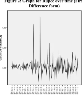
The Box-Jenkins methodology of building a model for any series begins with checking the series for stationarity. There are three properties of stationary, such as – no upward and downward trend, constant spread and no seasonality. A time series is said to be stationary if there is no systematic change in mean (no trend) over time, if there is no systematic change in variance (constant spread) and if periodic variation (seasonality) have been removed. Figure-1, represent the fact that data are non-stationary. A visual inspection clearly evidences that there is a trend in the data. It fails to prove the property (i). There is no seasonality in data and spreads are pretty constant. In this case property (ii) and (iii) have no problem. Thus to achieve stationary, this trend must be eliminated. For eliminating the trend, differencing method has been used. This method consists of subtracting the values of the observations from one another in some prescribed time dependent order. A first order difference transformation is defined as the difference between the values of two adjacent observations. By taking first order differences of a series with a linear trend, the trend disappears. Figure – 2 shows the result of first order differencing. This figure suggests that first order differencing has gone a long way to inducing stationary. The sample autocorrelation (ACF) or a correlogram and partial autocorrelation function (PACF) also helps to decide whether data are stationary or non stationary. Figure – 3 and 4 presents the ACF and PACF for the India

Figure 2: Graph for Rupee over time (First Difference form) O C T 20 02 M A Y 20 02 D E C 20 01 J U L 20 01 F E B 20 01 S E P 20 00 A P R 20 00 N O V 19 99 J U N 19 99 JA N 19 99 A U G 19 98 M A R 19 98 O C T 19 97 M A Y 19 97 D E C 19 96 J U L 19 96 F E B 19 96 S E P 19 95 A P R 19 95 N O V 19 94 J U N 19 94 JA N 19 94 A U G 19 93 M A R 19 93 O C T 19 92 M A Y 19 92 D E C 19 91 J U L 19 91 F E B 19 91 S E P 19 90 A P R 19 90 N O V 19 89 J U N 19 89 JA N 19 89 A U G 19 88 M A R 19 88 O C T 19 87 M A Y 19 87 D E C 19 86 J U L 19 86 F E B 19 86 S E P 19 85

Date: Month, Year

6.000 3.000 0.000 Va lu e DIFF(INDIA,1)

(Rupee) data on Figure- 1, before any differencing was performed. ACF plot clearly shows that the autocorrelations are large at many lags indicative of the lack of stationary. PACF plot illustrate, although not statistically significant, the PAC’s fail to die out, indicating that the data are not stationary.

Figure – 3: The ACF plot before any order difference 16 15 14 13 12 11 10 9 8 7 6 5 4 3 2 1 Lag Number 0.9 0.6 0.3 0.0 -0.3 -0.6 -0.9 AC F INDIA (Rupee) Lower Confidence Limit Upper Confidence Limit Coefficient

Figure – 4: The PACF plot before any order difference 16 15 14 13 12 11 10 9 8 7 6 5 4 3 2 1 Lag Number 0.9 0.6 0.3 0.0 -0.3 -0.6 -0.9 Part ial AC F INDIA (Rupee) Lower Confidence Limit Upper Confidence Limit Coefficient

Two tests called Augmented Dickey Fuller (ADF) and Phillips Perron (PP) test, which are actually help researcher to testing the stationary. The null hypothesis for ADF and PP test is that the data are not stationary i.e.

H 0: the data are not stationary

Versus H 1: the data are stationary

Table-1 shows the trend test results. The ADF (level) test statistics has numerical value 0.38881 with associated significance of 0.8233 which is greater than 0.05. So the null hypothesis is fail to reject and conclude that the non difference data is not stationary. After first differences the test statistics is now 106.049 with a significance level of 0.0000 which is less than 0.05. In terms of first differences, the null hypothesis is rejected and concludes that the first differences are trend stationary. Table -1 also shows the PP (level) test result. The test statistics has numerical value 0.38869 with associated significance of 0.8234 which is greater than 0.05. So the null hypothesis is fail to reject and conclude that the non difference data is not stationary. After running the first order difference the test statistics is now 110.807 with a significance level of 0.0000 which is less than 0.05. In terms of first differences, the null is rejected and conclude that the first differences are trend stationary.

Table 1: Trend test result

Test Method Statistic Prob.**

ADF Level Fisher

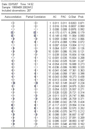
Chi-square 0.38881 0.8233 Choi Z-stat 0.92811 0.8233 1st Differ-ence Fisher Chi-square 106.049 0.0000 Choi Z-stat -9.97949 0.0000 PP Level Fisher Chi-square 0.38869 0.8234 Choi Z-stat 0.92830 0.8234 1st Differ-ence Fisher Chi-square 106.993 0.0000 Choi Z-stat -10.0262 0.0000 The correlogram analysis also performed to check the stationarity. This test indicated that underlying series was not stationarity. But the first difference of the series was stationarity.

Figure 5: The ACF and PACF plot before any order difference

DUMMY VARIABLE (PERIOD OF INTERVENTION):

The impact of economic, social and political stability helps the India’s Rupee exchange rate in the constant rise occurring at approximately last seventeen years (figure-1). Apart from the shifts caused by the devaluation and bombing, exchange rate appear to have a constant level as well as a constant variance, indicating a stationary series. The impact of the Cyclone and Bombing called an intervention. As the data consists with intervention two dummy variables have introduced. In this case, the first intervention period begins in the month of July 1991. On July 1991 Indian Rupee devaluated. The root causes of balance of payments crisis has been interference by the government in the free functioning of the foreign exchange market. Interference of any form requires some form of buffer stock such as foreign exchange reserve or gold to fall back upon during the hours of crisis. Another invention period begins in March 1993. The 1993 Mumbai bombings were a series of 13 bomb explosions that took place in Munbai (Bombay), India on March 12, 1993. The attacks were the most destructive

Figure 6: Correlogram of D(INDIA) First Difference

and coordinated bomb explosions in the country's history. The explosives went off within 75 minutes of each other across several districts of India's financial capital. The blasts were caused at prestigious and important buildings like Mumbai Stock Exchange, Air-India Building, and Hotel Sea Rock. Therefore, ‘Devaluation’ named as dummy_1 and ‘Bombing’ as dummy_2. The significant level of changes in exchange rate due to intervention must need to be considered. The period of interventions clearly showed in the figure 1 in July 1991 and March 1993, where the significant changes of exchange rate takes place. Exchange rate series have a statistically constant level before the intervention, followed by a statistically constant level after the intervention period is over. A constant shift in the level of a series can be modeled with a variable that is 0 until some point in the series and 1 thereafter. If the coefficient of the variable is positive, the variable acts to increase the level of the series, and if the coefficient is negative the variable acts to decrease the level of the series. Such variables are referred to as dummy variables. So, qualitatively, the rise in the exchange rate series can be modeled by a dummy variable with a positive coefficient.

Figure – 7: ACF plot with 1st _{order differencing} 16 15 14 13 12 11 10 9 8 7 6 5 4 3 2 1 Lag Number 0.9 0.6 0.3 0.0 -0.3 -0.6 -0.9 ACF DIFF(INDIA,1) Lower Confidence Limit Upper Confidence Limit Coefficient

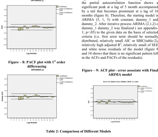
Figure – 8: PACF plot with 1st _order differencing 16 15 14 13 12 11 10 9 8 7 6 5 4 3 2 1 Lag Number 0.9 0.6 0.3 0.0 -0.3 -0.6 -0.9 Parti a l ACF DIFF(INDIA,1) Lower Confidence Limit Upper Confidence Limit Coefficient

The autocorrelation function shows a single significant peak at a lag of 5 month (figure 7); and the partial autocorrelation function shows a significant peak at a lag of 5 month accompanied by a tail that becomes prominent at a lag of 16 months (figure 8). Therefore, the starting model is ARIMA (5, 1, 5) with constant, dummy_1 and dummy_2. After iterative process ARIMA (2,1,2) c dummy_1 dummy_2 was finalized ( see appendix-1; p<.05) to the given data on the basis of selected criteria (i.e. first error term should be normally distributed, relatively small AIC or SBIC(table-2), relatively high adjusted R2_{, relatively small of SEE}

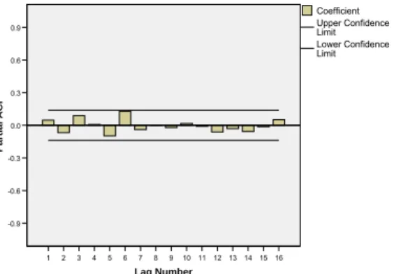
and white noise residuals of the model (figure 9 and 10 shows that there is no significant pattern left in the ACFs and PACFs of the residuals).

Figure – 9: ACF plot - error associate with Final ARIMA model 16 15 14 13 12 11 10 9 8 7 6 5 4 3 2 1 Lag Number 0.9 0.6 0.3 0.0 -0.3 -0.6 -0.9 ACF Lower Confidence Limit Upper Confidence Limit Coefficient

Error for INDIA from ARIMA, MOD_8, CON

Table 2: Comparison of Different Models

AIC SBIC Adj R2 SEE

ARIMA (5, 1, 5) c dummy_1 dummy_2 535.503 578.828 141.780 143.378 ARIMA (4,1,5) c dummy_1 dummy_2 533.403 573.395 141.763 144.641 ARIMA (3,1,5) c dummy_1 dummy_2 532.988 569.648 142.882 143.411 ARIMA (2,1,5) c dummy_1 dummy_2 530.942 564.269 142.886 143.414 ARIMA (2,1,4) c dummy_1 dummy_2 534.177 564.172 146.590 148.960 ARIMA (2,1,2) c dummy_1 dummy_2 531.391 554.720 147.492 141.628

Figure – 10: PACF plot - error associate with Final ARIMA model

16 15 14 13 12 11 10 9 8 7 6 5 4 3 2 1 Lag Number 0.9 0.6 0.3 0.0 -0.3 -0.6 -0.9 Par ti a l A C F

Error for INDIA from ARIMA, MOD_8, CON

Lower Confidence Limit Upper Confidence Limit Coefficient

Therefore, for forecasting the future values the following ARIMA model is selected-

2 _ 1 _ 2 2 1 1 2 2 1 1Z Z e e e dummy dummy Zt=μ+

φ

t−−

φ

t− −

θ

t−+

θ

t− + t+ + Or, 3.358 3.129 720 1.428 .852 1.526 .256+ 1− 2− 1+ 2+ + =

Z

₋

Z

₋

e

₋

e

₋

Z

t t t t t

Figure-11: Forecasting of exchange rate based on ARIMA (2, 1, 2) model

Date: Month, Year

AP R 2006 M AR 2 005 FE B 2 004 JA N 2 003 DE_{C 20} 01 NO V 2 000 OCT 1 999 SE_P 19 98 AU G 1 997 JU_{L 199} 6 JU N 1 995 M AY 1 994 AP R 19 93 MA R 1₉₉₂ FE B 19 91 JA N 1 990 DE C 19 88 NO V 1 987 OCT 1 986 SE P 1985 V al ue I ndi a ( R upee) exchange r at e 80 70 60 50 40 30 20 10 0 OBSERVED PREDICTED EXPONENTIAL SMOOTHING MODEL:

Table – 3 illustrate the result of the exponential smoothing model of the India (Rupee) exchange rate produced by SPSS. The value of α and

γ

are α = 1.00000,

γ

= 0.0000 with the minimum SSE of 198.97987.

Table 3: Results of the Exponential Smoothing model with α and

γ

Smallest Sums of Squared Errors

Series Model rank Alpha (Level) Gamma (Trend) Sums of Squared Errors INDIA 1 1.00000 .00000 198.97987 2 .99000 .00000 199.04500 3 .98000 .00000 199.15105 4 .97000 .00000 199.29813 5 .96000 .00000 199.48636 6 .95000 .00000 199.71591 7 .94000 .00000 199.98697 8 .93000 .00000 200.29976 9 .92000 .00000 200.65454 10 .91000 .00000 201.05161 Smoothing Parameters Series Alpha

(Level) Gamma (Trend) Squared Errors Sums of errorDf INDIA 1.00000 .00000 198.97987 206 Shown here are the parameters with the smallest Sums of Squared Errors. These parameters are used to forecast.

Figure -12 plots the observed and forecasted India (Rupee) exchange rate data and it is evident that optimal model generate excellent fit.

Figure-12: Forecasting of exchange rate based on exponential smoothing model

O C T 2 0 0 2 D E C 2 0 0 1 J U L 2 0 0 1 F E B 2 0 0 1 S E P 2 0 0 0 A P R 2 0 0 0 N O V 1 9 9 9 J U N 1 9 9 9 J A N 1 9 9 9 A U G 1 9 9 8 O C T 1 9 9 7 D E C 1 9 9 6 J U L 1 9 9 6 F E B 1 9 9 6 S E P 1 9 9 5 A P R 1 9 9 5 N O V 1 9 9 4 J U N 1 9 9 4 J A N 1 9 9 4 A U G 1 9 9 3 O C T 1 9 9 2 D E C 1 9 9 1 J U L 1 9 9 1 F E B 1 9 9 1 S E P 1 9 9 0 A P R 1 9 9 0 N O V 1 9 8 9 J U N 1 9 8 9 J A N 1 9 8 9 A U G 1 9 8 8 O C T 1 9 8 7 D E C 1 9 8 6 J U L 1 9 8 6 F E B 1 9 8 6 S E P 1 9 8 5

Date: Month, Year 70 60 50 40 30 20 10 Val u e I ndi a(Rupee) exchange r a te YHAT (PREDICTED) INDIA (OBSERVED)

NAÏVE 1 AND NAIVE 2 MODEL:

Naïve 1or no change model says that the forecast for June 2006 should equal to the value for June 2005. Lag12 for September 1986 is equal to the observed value for September 1985 here; the value of the variable Lag12 thus represents that forecasted value for September 1986 under the naïve 1 model. The residuals (variable name resid) are simply INDIA-Lag12. Naïve 2 model assumes that the growth rate in the previous period applies to the generation of forecasts for the current period. To run the Naïve 2 model two variables Lag12 and lag24 were created. Appendix -3 indicates that there is a large amount of data loss when applying the Naïve 2 model for a given data set. The forecasted values was calculated by using the

following formula, YHAT=

]

24

/

)

24

12

(

1

[

*

12

lag

lag

lag

lag

+

−

and the

residuals are computed as: Resid = (INDIA

-YHAT).The detail result of Naïve 2 models are available in appendix-3.

VI. COMPETING MODLES

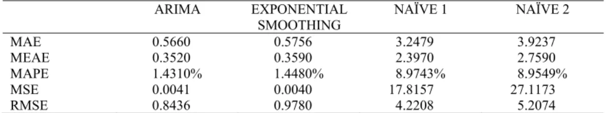
An important objective of this study is to be search the best predictive performance model among all the competitive models. Table -4 shows the summary result for all four models. Mean Absolute Error (MAE), Median Absolute Error (MEAE), Mean Absolute Percentage Error (MAPE), Mean Square error (MSE), Root mean square error (RMSE) are some of the frequently used measures of forecast adequacy. The rule of thumb is the smaller MAE, MEAE, MAPE, MSE and RMSE, the better is the forecasting ability of that model. The MAE, MEAE, MAPE, MSE and RMSE associated with ARIMA model is the smaller, compare with other three models. Therefore, it is proposed that ARIMA model is the best among all these models.

Table 4: Comparison of models

ARIMA EXPONENTIAL

SMOOTHING NAÏVE 1 NAÏVE 2

MAE 0.5660 0.5756 3.2479 3.9237 MEAE 0.3520 0.3590 2.3970 2.7590 MAPE 1.4310% 1.4480% 8.9743% 8.9549% MSE 0.0041 0.0040 17.8157 27.1173 RMSE 0.8436 0.9780 4.2208 5.2074 VII. CONCLUSION

This study has assessed comprehensively and systematically the predictive capabilities of the exchange rate forecasting models. To obtain the generality of the empirical results, ARIMA, Exponential Smoothing, Naive1 and Naïve 2 model have been compared. Some of the frequently used measures of forecast adequacy such as MAE, MEAE, MAPE, MSE and RMPE were used to evaluate the forecast performance of the chosen models. Based on the result of this study it can conclude that exchange rates do not exhibit a random walk and it is quite possible to build a model for it, although slightly difficult. This study reveals the fact that ARIMA methodology produces superior results than other three models. The main contribution of this study is in evaluating the forecast performance of the various time series models in a comprehensive and systematic way. Empirical results in this study will also pave the way for future research.

REFERENCES

[1] Bilson, J.F.O: “Rational expectations and the exchange rate”, in J.A. Frankel and H.G. Johnson (eds.), The Economics of Exchange Rate (Reading, Mass, Addison-Wesley), pp 75-96. (1978)

[2] Box, G., & Jenkins, G.: Time Series Analysis, Forecasting, and Control. San Francisco, California: Holden day. (1976) [3] Brooks. C: Introductory Econometrics for

Finance. UK: Cambridge. (2003)

[4] Cao R., García Jurado I., Gonzalez Manteiga W., Prada Sanchez J.M. and Febrero-Bande M., “Predicting using Box-Jenkins, nonparametric and bootstrap techniques” Technometrics 37, 303-310. (1995)

[5] Chinn, Menzie D. and Meese, Richard A.: “Banking on Currency Forecasts: How

Predictable is Change in Money?” Journal of International Economics, 38, pp.161-178. (1995)

[6] Dornbusch, R.: “Expectations and exchange rate dyanamics”, Journal of Political Economy, 84, pp 1161-1176, (1976).

[7] Frankel, J.: “On the mark: A theory of floating exchange rates based on real interest differentials”, American Economic Review, 69, pp. 610-622. (1979)

[8] Hamilton, J, Time Series Analysis, Princeton, New Jersey: Princeton University Press, 22. (1994)

[9] Hooper, P and J.Morton: “Fluctuations in the dollar: A model of nominal and real exchange rate determination” Journal of International Money and Finance, 1, pp. 39-56. (1982).

[10] Imad A. Moosa, “Exchange Rate Forecasting; techniques and applications” Macmillan Business, London (2000). [11] International Monetary Fund: International

Financial Statistics. Various issues, January 1987 to August 2006, Washington.

[12] John Faust, John H. Rogers, Jonathan H. Wright “Exchange rate forecasting: the errors we’ve really made”, Journal of International Economics, 60,pp 35-59. (2003)

[13] Lindsay I. Hogan, “A comparision of alternative exchange rate forecasting models”,Bureau of agricultural Economics, Canberra ACT 2601.

[14] Lutz Lillian and Mark P. Taylor, “Why it is so difficult to beat random walk forecast of exchange rates?”, Journal of International Economics,60,pp85-107. (2003)

[15] MacDonald, Ronald and Ian Marsh: “On Fundamentals and Exchange Rates: A Casselian Perspective,” Review of Economics and Statistics 79(4): pp.655-664. (1997)

[16] Mark, Nelson C.: “Exchange Rates and Fundamentals: Evidence on Long-Horizon Predictability”. American Economic Review, 85, pp.201-18. (1995)

[17] Mary E. Gerlow and Scott H. Irwin, “The performance of exchange rate forecasting models: an economic evaluation”, Applied Economics, 23, 133-142. (1991)

[18] McDonald, R. and M. P. Taylor: “Exchange Rates Economics: A Survey,” IMF Staff Papers, 39, pp.1-57. (1992)

[19] Meese, R. A. and K. Rogoff: “Empirical Exchange Rate Models of the Seventies: Do They Fit Out of Sample?” Journal of International Economics, pp.3-24. (1983) [20] Meese, R. A. and K. Rogoff: “The

Out-of-Sample Failure of Empirical Exchange Rate Models: Sampling Error or Misspecification?” in Exchange Rate and Interantional Macroecomics, J. Frenkel ed., University of Chicago Press, Chicago, pp. 67-112. (1983)

[21] Tambi, K. Mahesh: Forecasting Exchange Rate: A Univariate Out-of-Sample Approach (Box-Jenkins Methodology), The ICFAI Journal of Bank Management, IV, 60-74. (2005)

[22] Yiu-Man Chan: Forecasting Tourism: A Sine Wave Time Series Regression Approach, Journal of Travel Research, Vol. 32, No. 2, pp 58-60. (1993)

APPENDIX-1 Parameter Estimates

ARIMA (2, 1, 2) with constant and dummy_1 and dummy_2 result Esti-mates Std Error t Approx Sig Non- Seasonal Lags AR1 1.526 .111 13.799 .000 AR2 -.852 .110 -7.739 .000 MA1 1.428 .147 9.690 .000 MA2 -.720 .147 -4.898 .000 Regression CoefficientsDummy_1 3.129 .576 5.436 .000 dummy_2 3.358 .576 5.834 .000 Constant .256 .053 4.791 .000

APPENDIX-2

Lagged values and residuals values of Naïve 1 model

APPENDIX-3

Forecasted and residuals values from the Naïve 2 model