Middlesex
University
Middlesex University Research Repository:
an open access repository of
Middlesex University research
Mawutor Ahadzi, Gershon. 2006. Techniques for imaging small
impedance changes in the human head due to neuronal depolarisation.
Available from Middlesex University's Research Repository.
Copyright:
Middlesex University Research Repository makes the University's research available electronically.
•
Copyright and moral rights to this thesis/research project are retained by the author and/or other copyright owners. The work is supplied on the understanding that any use for commercial gain is strictly forbidden. A copy may be down loaded for personal, non-commercial, research or study without prior permissio'n and without charge. Any use of the thesis/research project for private study or research must be properly acknowledged with reference to the work's full bibliographic details. This thesis/research project may not be reproduced in any format or medium, or extensive quotations taken from it, or its content changed in any way, without first obtaining permission in writing/from the copyright holder(s).
If you believe that any material held in the repository infringes copyright law, please contact the Learning Resources at Middlesex University via the following email address: .
TECHNIQUES FOR IMAGING SMALL IMPEDANCE
CHANGES IN THE HUMAN HEAD DUE TO
NEURONAL DEPOLARISATION
In Collaboration with
University College London A thesis submitted to Middlesex University in partial fulfilment of the
require!llents for the degree of
Doctor of Philosophy
Gershon Mawutor Ahadzi
School of Health and Social Sciences Middlesex University
P
\3
'2.J::lq
t \
<_
:
:slt~'
,
~-~IODLESEX'~
_
... e:J ' ..
l~.!
..
;~~_~:~~_~~~.
Acce:;!;;"'n No. Class No.o
S~q
Y/"1"2;2 '.
~;:1'~'~(;-::~-5
L,
.--..
.1hL~.
___
Special I! / ' Collection LV"TABLE OF CONTENTS
List of figures ... vii
List of tables ... xiii
List of abbreviations ... xv List of symbols ... xvll Acknowledgments ... xviii Declaration ... xix Abstract ... 1 Chapter 1 ... 3
Introduction and Review ... 3
1.1 Motivation ... 3
1.2 Overview ... 4
1.2.1 Origin of brain signals ... 4
1.2.2 Bioelectric and biomagnetic signals ... 9
1.2.3 How does current flow through the brain? ... 10
1.2.4 Brain Imaging Systems ... 13
1.2.5 Integrated Imaging Systems and their applications ... ; ... 36
1.2.6 Electrical properties of tissue ... ~ ... 38
1.2.7 Resistance changes in the brain and their visibility using ElT ... .42
1.2.8 Ionic changes and cell swelling during neuronal activity ... .48
1.2.9 Current injection and voltage measurement ... 51
1.2.10 Electrode Protocols ... 56
1.3 Scope of Work ... 60
1.4 Summary ... 60
1.5 Objective of research ... 61
Chapter 2 ... 63
2.1. Modelling in ElT ... 63
2.1.1. 2-D models ... -... 63
2.1.2. 3-D models ... 65
2.1.3. Models of the head ... 65
2.1.4. Modelling in EEG ... 68
2.1.5. Anisotropy ... 70
2.2. The forward problem ... 70
2.3. Mathematical formulation ... 72
2.4. Uniqueness, ill-posedness and ill-condition ... 74
2.5. Volume Source in a Homogeneous Volume Conductor ... 75
2.6. Volume Source in an Inhomogeneous Volume Conductor ... 76
2.7. Quasistatic Conditions ... 78
2.8. Sununary ... 78
Chapter 3 ... 80
Neuromagnetic Field Strength Outside The Human Head Due To Impedance Changes From Neuronal Depolarisation ... 80
3.1 Introduction ... 80
3.1.1 Background ... 80
3.1.2 Purpose of study ... 82
3.1.3 Proposed Imaging Sensor ... 83
3.1.4 Design ... 84
3.2 Methods ... 85
3.2.1 Volume Conductor Model. ... 85
3.2.2 The source model ... 86
3.2.3 Current Injection ... 87
3.3 Mathematical Principles ... 88
3.3.1 Current Density Estimation ... 88
3.3.2 Magnetic Field Estimation ... 89
3.4 Simulation ... 91
3.5 Results ... 93
3.5.1 Estimated Magnetic Field ... 93
3.5.2 V mation of magnetic field ... 96
3.6 Discussion ... 98
3.6.1 Summary of results ... 98
3.6.2 Technical issues ... 98
3.6.3 Would the changes be detectable with current MEG technology? ... 100
3.6.4 Does this modelling suggest an advantage over EEG recording? ... .101
Chapter 4 ... 103
Modelling Of Electrode Pairs For Optimal Current Density Estimation In The Visual Cortex And Optimal Voltage Change Measurement ... 1 03 4.1 Introduction ... 103 4.1.1 Background ... 103 4.1.2 Purpose of study ... 1 06 4.1.3 Design ... 106 4.2 Method ... 107 4.2.1 The Meshes ... 107
4.2.2 The source model ... 109
4.2.3 Current injection and electrode model ... 11 0 4.3 Mathematical principles ... 111
4.3.1 Simulations and Analysis ... 113
4.3.2 Experimental validation ... 115
4.4 Results ... 117
4.4.1 Baseline surface potential ... 117
4.4.2 Simulated and experimental homogeneous sphere ... 117
4.4.3 Simulated and experimental three layer head tank ... 118
4.4.5 Three layer head ... 118
4.4.6 Four layer head ... 119
4.4.7 Current density ... 120
4.4.8 Validation by human Experiment ... .122
4.4.9 Best Recording electrodes ... 123
4.5 Discussion ... 124
4.5.1 Sutnmary ... 124
4.5.2 Technical Issues ... 124
Chapter 5 ... 130
Effect of variations in skull conductivity, shape and size of V1 on current density distribution in the brain and baseline surface potential ... 130
5.1 Introduction ... 130 5.1.1 Purpose ... 131 5.1.2 Background ... 132 5.1.3 Design ... 137 5.2 Method ... : ... 141 5.2.1 Head Model ... 141
5.2.2 Creation of a 3D electrode protocol file ... 144
5.3 Results ... 14 7 5.3.1 Percentage change in current density ... 147
5.3.2 Percentage change in current density ... .156
5.3.3 Baseline boundary voltages and changes ... 156
5.3.4 Changes in boundary voltages for different local conductivity changes ... .164
5.3.5 Non uniformity ratio ... 164
5.3.6 Multiple current injection ... 167
5.4 Discussion ... 169
5.5 Conclusion ... 170
Chapter 6 ... 172
magnetic field estimation of the realistic head using eidors ... 172
6.1 Introduction ... 172
6.1.1 Purpose ... 174
6.1.2 Design ... 174
6.2 Method ... 175
6.2.1 Volume conductor and source models ... 175
6.2.2 The electrode protocol ... 177
6.2.3 The simulation ... 178
6.3 Results ... 179
6.3.1 Baseline magnetic fields ... 179
6.3.2 Percentage Changes in magnetic field ... 181
6.4 Discussion ... 188
6.5 Is there any advantage ... 190
6.6 Observations ... 191
Chapter 7 ... 193
conclusions and suggestions for future work ... 193
7.1 Summary of work done ... 193
7.1.1 Research question ... 195
7.1.2 Review ... 195
7.1.3 Multi-modality ... 196
7.1.4 Optimal electrode protocoL ... 198
7.1.5 Effect of conductivities on surface potential changes ... 200
7.1.6 Effect of conductivities off-scalp magnetic field changes ... 201
7.2 Suggestions ... 201
7.2.1 Methods of increasing current density in the brain ... 201
7.2.2 Development of accurate forward problem ... 202
7.2.3 Best optimal current pattern using distinguishability approach ... .204
-Geselowitz' Sensitivity Theorem ... 209
Appendix B ... 211
Spectral noise density ... 211
References ... 213
List of figures
Figure 1-1: The human brain ... 4
Figure 1-2: The structure of a typical neurone ... 5
Figure 1-3: Resting potential curve ... 6
Figure 1-4: The action potential of a nerve fibre ... 8
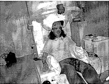
Figure 1-5: A subject in a typical magneto encephalogram (NTF 275) ... 24
Figure 1-6: Magnetic Fields ... 25
Figure 1-7 Magnes 3600 248 l\1EG Channels ... 26
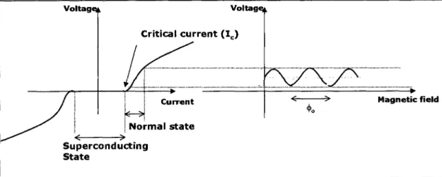
Figure 1-8: Principles of SQUID operation ... 29
Figure 1-10: SQUID sensor electronics ... 31
Figure 1-11: Flux Transfonners a: an axial first order gradiometer which measures
a::
(approximately Bz at the lower loop) b: second order series axial gradiometer ... 32Figure 1-12: Systems already integrated are shown with thick lines, the dotted is currently under study ... 37
Figure 1.13. The flow of externally applied current inside and outside an axon and across its membrane (a) during the resting state and
(b)
during depolarisation. More current flows through the intracellular space during depolarisation (Liston, 2003) ... .47Figure 1.14: Mechanisms of impedance change within the brain (Tidswell et al., 2001) ... 50
Figure 1.15: Neighbouring method of impedance data collection. The first four voltage measurements for the set of 13 measurements are shown. B shows another set of 13 measurements, which is obtained by changing the current feeding electrodes ... 52
Figure 1.16: Opposite method of impedance data collection ... 53
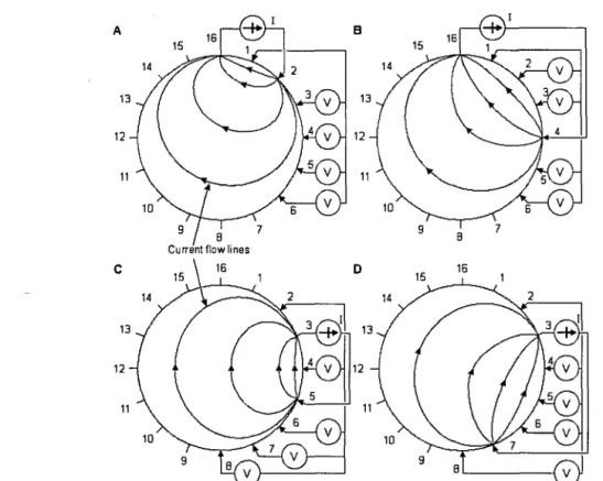
Figure 1.17: Cross method of impedance data collection. The four different steps of this approach are illustrated in A through D ... 54
Figure 1.18: Adaptive method of impedance data collection ...•... 55 Figure 1.19: The international 10-20 system seen from the left side of the head (A) and B
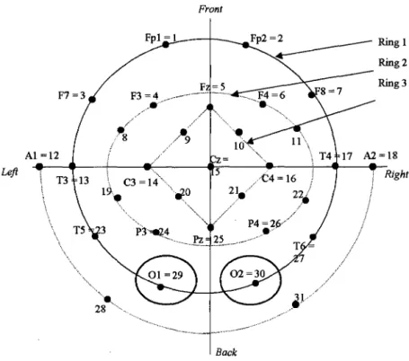
-frontal, Fp - frontal polar, 0 -occipital. In (C) is the location and nomenclature of the intermediate 10% electrodes, as standardised by the American Electroencephalographic Society ... 56 Figure 1.20: Positions of electrodes. Each black spot represents an electrode. The black
label gives the electrode code in the 10-20 system, the red number is the electrode reference number used in this work. ... 59 . Figure 3-1: ElT system for current injection ... 83 Figure 3-2: (a) An approximation of the realistic head to a fourshell sphere model
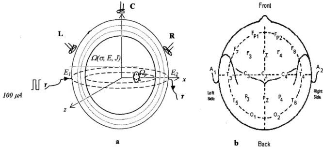
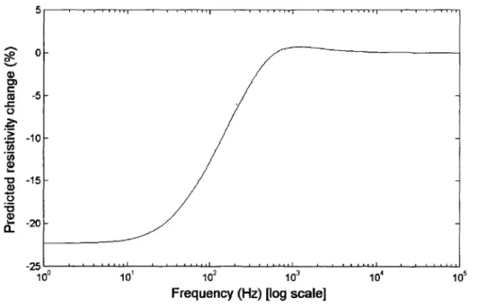
showing points of current injection El and E2. R, C, and L are the locations of typical SQUID sensors for the measurement of the magnetic field. The gray region Qp is a collection of nodes indicating a region in the brain where the neurons are firing and the conductivity is cr'. The conductivity at other regions within the volume Q is cr. (b) The EEG 10-20-system showing the relationship between the location of an electrode and the underlying area of cerebral cortex. " ... 85 Figure 3-3: Predicted change in resistivity versus frequency during neuronal depolarisation .... 87 Figure 3-4: The depolarised region is denoted by Qp whereas the remaining volume is
labelled Qu' The entire volume conductor is represented by Q. The point at which the magnetic field is estimated is B. The position vectors of the source (node) and point of measurement are respectively raa and ra respectively from a fixed origin O. The distance between the source and P is
Ira - t;,al.
Ja denotes the current density at a node.uE ri, j, k} ... 89 Figure 3-5: Fractional magnetic field change during evoked response with respect toposition for homogeneous sphere fine mesh model The x-axis denotes the distance of the centre of the depolarised region from the centre of the head ... 96 Figure 3-6: Fractional magnetic field change from baseline with respect to position for
fourshell fine mesh model. The x-axis denotes the distance of the centre of the depolarised region from the centre of the head ... 97
Figure 3-7: A MatLab interpolated SURF plot of current density on an 80x80 grid (A m-l
in the plane of two bipolar electrodes applying 1~ on the surface of a) a
homogenous sphere of conductivity crbrain and b) a 4-shell sphere. The x- and y-axes are pixel numbers (Liston, 2003) ... 100 Figure 4.2: A - The brain region showing the primary visual cortex as Brodmann area 17
and B shows the modelled realistic head with Vl using FEM ... l09 Figure 4.4: Illustration of ElT acquisition principle: small curreht injected through a pair
of electrodes, and the surface potential (V) measured via another pair. This
process is repeated for different injection-measurement combinations ... 114
Figure 4.5A: The homogeneous spherical tank phantom, shown for clarity without the
presence of the shell to represent the skull. The protruding leads are the connections to various positions ... 116 Figure 4.5B: The head shaped tank phantom shown with the two halves separated and a
human skull inside ... 116 Figure 4.6. Mean current density in Vl for an injected current through electrodes 29 and
30 paired with other electrodes. The horizontal axis refers to the number assigned to each electrode as modelled ... 121 Figure 4.7 Comparison between measured base voltages on human and simulated base
voltages from 4 shell realistic mesh (skull conductivity 17.5mS/m). The Blue is injection pair 1 (23-30) and red is injection pair 2 (27 -29) ... 122 Figure 5.1: The three selected morphologies of the primary visual cortex a) inclined b)
elongated c) blob ... 139
Figure 5.2: The element faces on the surfaces of the four parts of the full, layered head
mesh a) the scalp, b) the skull, c) the CSF and d) the brain region. The scalp
.
region contains 10,078 nodes, the skull region 6,325 nodes, the CSF region 2,064 nodes and the brain region 6,702 nodes ... 142Figure 5.3: The nodal clouds describing a) the head-shaped mesh with skull compartment, b) the fours hell mesh and c) the full, layered head mesh. The different tissues are colour-coded as shown in the key ... 143 Figure 5.5a. Plot of current density and percentage change in mean current density in V1
as a function of skull conductivity for morphology 1, for volumes 1 and 2 of the primary visual cortex ... 148 Figure 5.5b. Plot of current density and percentage change in mean current density in V1
as a function of skull conductivity for morphology 1, for volumes 3 and 4 of the primary visual cortex ... 149 Figure 5.6a. Plot of current density and percentage change in mean current density in V1
as a function of skull conductivity for morphology 2, for volumes 1 and 2 of the primary visual cortex ... ; ... 151 Figure 5.6b. Plot of current density and percentage change in mean current density in V1
as a function of skull conductivity for morphology 2, for volumes 3 and 4 of the primary visual cortex ... 152 Figure 5.7a. Plot of current density and percentage change in mean current density in V1
as a function of skull conductivity for morphology 3, for volumes 1 and 2 of the primary visual cortex ... 154 Figure 5.7b. Plot of current density and percentage change in mean current density in V1 .
as a function of skull conductivity for morphology 3, for volumes 3 and 4 of the primary visual cortex ... 155 Figure 5.8a Plot of baseline boundary voltages for different conductivities with respect to
index of measurement electrode pairs for morphology 1 for sizes 1 and 2 ... 158 Figure 5.8b Plot of baseline boundary voltages for different conductivities with respect to
index of measurement electrode pairs for morphology 1 for sizes 3 and 4 ... .159 Figure 5.9a Plot of baseline boundary voltages for different conductivities with respect to
index of measurement electrode pairs for morphology 2 for sizes 1 and 2 ... 160
Figure 5.9b Plot of baseline boundary voltages for different conductivities with respect to index of measurement electrode pairs for morphology 2 for sizes 3 and 4 ... 161 Figure 5.10a Plot of baseline boundary voltages for different conductivities with respect
to index of measurement electrode pairs for morphology 3 for sizes 1 and 2 ... 162 Figure 5.1 Ob Plot of baseline boundary voltages for different conductivities with respect
to index of measurement electrode pairs for morphology 3 for sizes 3 and 4 ... 163 Figure 5.11 a. Non-uniformity ratio plots for different electrode combinations for a fixed
conductivity of 17.5 mSm-1 ....•...•..•...•••.•..•...••....•.•..•.•...•...•..••....••....•...•... 166
Figure 5.11 b Non-uniformity ratio plots for different electrode combinations with variation over skull conductivity ... 166 Figure 5.12a: Mean current density in V1 for independent current injection pairs as a
function of conductivity ... 167 Figure 5.12b. Mean current density in V1 for multiple current injection where the injected
currents are 1 00 ~ each and using morphology 1.. ... 168 Figure 6-1: The homogeneous and head sphere fine head models. The homogeneous head
model has 24,734 nodes whereas the sphere fine has 36,000 nodes ... 176 Figure 6-2: The fourshell head model with 42,093 nodes. The conductivity values of the
different shells (scalp, skull, cerebrospinal fluid, and brain) are as specified in table 4.1, section 4.2.1 ... 176 Figure 6-3: The red-circles (0) denote electrode positions for current injection whereas
the blue crosses (+) are 1-cm radially away from points of current injection where the Squids are located for estimating the baseline magnetic field. The green points
(*) are the sensor locations L, C and R (used in chapter 3) Both axes have units in meters ... 177 Figure 6.4: Baseline magnetic field for fourshell head modeL The horizontal axis refers to
the location of the SQUIDs position ... 179 Figure 6.5: Baseline magnetic field for realistic head modeL The horizontal axis refers to
Figure 6.7: Realistic head percentage changes in magnetic field from baseline as a function of position of SQUIDs, for morphology 1 and sizes 3 and 4 ... 183
Figure 6.8: Realistic head percentage changes in magnetic field from baseline as a
function of position of SQUIDs, for morphology 2 and sizes 1 and 2 ... 184
Figure 6.9: Realistic head percentage changes in magnetic field from baseline as a
function of position of SQUIDs, for morphology 2 and sizes 3 and 4 ... 185
Figure 6.10: Realistic head percentage changes in magnetic field from baseline as a
function of position of SQUIDs, for morphology 3 and sizes 1 and 2 ... 186
Figure 6.11: Realistic head percentage changes in magnetic field from baseline as a
function of position of SQUIDs, for morphology 3 and sizes 3 and 4 ... .187 Figure B-1: Spectral noise density for a SQUID as a function of frequency.
Source(MEG-EEG Centerat Pitie-Salpetriere Hospital, 2000) ... 211
List of tables
Table 1-1: Reported values for the resistivity of grey matter ... 39
Table 3-1: Baseline magnetic field for fine mesh ... 94
Table 3- 2: Maximum magnetic field change from baseline field strength for fine mesh ... 94
Table 3-3: Maximum percentage change from baseline magnetic field for fine mesh ... 94
Table 3-4: Baseline magnetic field for medium mesh ... 95
Table 3- 5: Maximum magnetic field change from baseline field strength for medium mesh ... 95
Table 3.6: Maximum percentage change from baseline magnetic field for medium mesh ... 95
Table 4.1: Conductivity values of the different layers of the head (Oostendorp and Debelke, 2000) ... 1 08 Table 4.2: listed are the three meshes, the number of nodes and elements and the ratio of largest-to-smallest element size in each head shape. This ratio is a measure of their quality and a smaller value is desirable ... .1 08 Table 4.3: Comparison between simulated and experimental baseline voltages for homogeneous spherical tank ... : ... 117
Table 4.4: Comparison between simulated and experimental baseline voltages for three-layer head tank Oatex tank) for the best pairs of electrodes ... 118
Table 4.5: Best pairs for recording surface potential and injecting current for the 3 layer head ... 119
Table 4.6: Best pairs for recording surface potential and injecting current for the 4 layer head ... 120
Table 5.1: Specific conductivity of bone. (n.a : not applicable) ... 133
Table 5.2: Computed volumes of the left and right hemisphere of Vl together with the total mean volume ... 140
Table 5.3: Listed are the three meshes used in this chapter, the number of nodes and elements in each and the ratio of largest-to-smallest element size in each, a measure of their quality. A smaller value is desirable ... 143 Table 5.4 Computed percentage change in mean current density for a 1 % local change V1
over variations in skull conductivity and volume ofV1 ... 156 Table 5.6: Percentage change in boundary voltages with respect to local conductivity and
skull conductivity ... 164 Table 6.1 Range of baseline magnetic fields across SQUID sensor locations for two types
of current injections protocol: (DMO - Diametrically Opposed and BCE Best Current Injection Electrodes) ... 181 Table 6.5 Computed percentage change baseline magnetic field for a 0.6% local change
inV1 over SQUID locations ... 189 Table 6.6 Computed percentage change baseline magnetic field for a 1 % local change
in V1 over SQUID locations ... 189 Table 6.7 Computed percentage change baseline magnetic field for a 1.6% local change
in V1 over SQUID locations ... 189
ACT BCE BEM BOLD BREIT CAP CAT CBV CSF CT DC (dc) DOM EcoG EEG EIDORS ElT EITS EP FEM fMRI Hb Hb02 I-DEAS lEG IPT MaTOAST MEG MCS List of abbreviations
Applied Current Tomography Best Current-injection Electrode Boundary Element Method
Blood Oxygenation Level Dependent
BOLD-Related Electrical Impedance Tomography Compound Action Potential
Computerised Axial Tomography Cerebral Blood Flow
Cerebrospinal Fluid Computed Tomography Direct Current
Diametrically Opposed Method Electrocortigogram
Electroencephalography
Electrical Impedance and Diffuse Optical Reconstruction Software Electrical Impedance Tomography
Electrical Impedance Tomographic Spectroscopy Evoked Potential
Finite Element Method
functional Magnetic Resonance Imaging Hemoglobin
Oxygenated Hemoglobin
Integrated Design and Analysis Software Immediate-Early Gene
Industrial Process Tomography
Matlab Time-resolved Optical Absorption and Scattering Tomography
Magnetoencephalography Multiple Current Source
MRI NIRS NURBS PET RNA rCBF SCS SEP SPM SQUIDS SPECT SVD SVS TOAST VEP Vl
Magnetic Resonance Imaging Near Infra Red Spectroscopy Non-Uniform Rational B-Spline Positron Emission Tomography Ribonucleic Acid
regional Cerebral Blood Flow Single Current Source
Somatosensory Evoked Response Statistical Parametric Mapping
Superconducting QUantum Interference Devices Single Photon Emission Computerised Tomography Singular Value Decomposition
Single Voltage Source
Time-resolved Optical Absorption and Scattering Tomography Visual Evoked Potential
Primary Visual Cortex
List of symbols (j' Conductivity E Electric Field
rp
Electric Potential H Magnetic FieldJ
Current Density V Voltage A Sensitivity Matrix Z Impedance I Current ~,<l> Electric Potential M Number of Measurements N Number of Pixels/Nodes S Support Matrix v elemental volume r Position Vector r Radial PositionAcknowledgments
I wish to express my sincere appreciation to my Director of Studies, Professor Richard H. Bayford, host supervisor Dr David S. Holder and co-supervisor Dr Robert Ettinger for their indefatigable effort in directing me to complete this study. I am very much indebted to them for their professional guidance.
Special thanks to my colleagues Dr Adam Liston from whom I had a lot of encouragement at the initial stage of the project; Ori Gilad, who tutored and made proud of using MatLab as my everyday programming tool. Lior Horesh, I say a big thank you for assisting me to understand the lengths of codes in the forward solution.
To God be the Glory!
•
Sponsors: University of Ghana, Legon-Accra, Ghana
Declaration
I carried the research work presented in this thesis under the supervision of Prof. Richard Bayford, the Director of Studies together with my external supervisors Dr David Holder (Medical Physics and Bioengineering Department, University College London) and Dr Robert Ettinger (School of Computing Science, Middlesex University). The laboratory and experimental validation work reported was done pardy at the Clinical Neurophysiology Department of University College London Hospitals and the Medical Physics and Bioengineering Department, University College London.
Many members of the ElT group both past and present in one way or the other contributed tremendously to this research work. The experimental section was done in collaboration with Od Gilad who is also a PhD student working on experimental set ups for human studies, which could be used to verify some of my predictions from the models I developed. Adam Gibson - development of an analytical homogenous head model for a conduction sphere, and Adam Liston who developed the fourshell head model which were used extensively in the first part of this research work. Andrew Bagshaw helped me in the initial modification of and debugging the 3D MaTOAST code.
The realistic head model meshes were by courtesy of Andrew Tizzard and Richard Bayford. I used MatLab to develop and implement codes for the simulation. However, a number of functions and modules were adopted from EIDORS with the singular help of Lior Horesh.
Refereed Paper as a Result of this work!
Ahadzi, G. M., Liston, A. D., Bayford, R. H., & Holder, D. S. 2004, "Neuromagnetic field strength outside the human head due to impedance changes from neuronal depolarization", Physio!. Meas., vo!. 25, no. 1, pp. 365-378.
Conference Papers & Posters as a Result of this work
1. Ahadzi, G. & Bayford RH 2005, "Current density distribution in the brain and baseline scalp potential- How are they influenced by variations in skull and local conductivity, shape and size of Vl?" Poster Presentation - Inauguration and opening of Biomedical Laboratory Centre, Middlesex University.
2. Ahadzi, G. & Bayford, R. 2005, "Are there any changes in the mean current density in the visual cortex due to variations in the conductivity of the human skull?" Abstract of Research in Practice, Institute of Social & Health Research, School of Health & Social Sciences, Middlesex University, London,June 24 2005, pp.l0.
3. Ahadzi, G. & Bayford, R. 2006, "Is magnetic recording of ElT the holy grail of imaging small and fast impedance changes in the human brain?" Abstract of Research in Practice, Institute of Social &
Health Research, School of Health & Social Sciences, Middlesex University, London, June 23 2006, pp.15
4. Ahadzi, G., Gilad, 0., Horesh, L., Bayford, R., & Holder, D. 2004, "An ElT electrode protocol for obtaining oprimal current density in the primary visual cortex", Proceedings of the XII
Intern.Conf.Electrical Bio-Impedance and ElT, Gdansk, Poland, vol. II, pp. 621-624.
5. Ahadzi, G., Liston, A., Bayford, R., & Holder, D. 2003, "Would SQUID measurement of magnetic fields be a better way to do ElT imaging of fast electrical brain activity?" Proceedings of 4th International Conference on Biomedical Applications of ElT, University of Manchester Institute of Technology, Manchester.
6. Gilad, 0., Ahadzi, G., Bayford, R, & Holder, D. 2004, "Near DC conductivity change measurement of fast neuronal activity during human VEP", Proceedings of the XII International Conference Electrical Bio-Impedance and ElT, Gdansk, Poland, vol. I, pp. 279-282.
7. Gilad, 0., Ahadzi, G., Bayford, R., & Holder, D. 2004, "Near DC resistivity change measurement of fast neuronal activity during human visual evoked potentials (VEP)", Poster Presentation, Medical Physics & Bioengineering Department, University College London.
8. Gilad, 0., Horesh, L., Ahadzi, G., Bayford, R., & Holder, D. 2005, "Could synchronized neuronal activity be imaged using low frequency electrical impedance tomography?" Scientific Abstracts of the 6th International Conference on Biomedical Applications of ElT, Univ.CoI.London, June 22 - 24 2005.
9. Gilad, 0., Horesh, L., Ahadzi, G., Bayford, R., & Holder, D. 2005, "Towards imaging synchronised neuronal activity using low frequency electrical impedance tomography", Poster Presentation, Medical Physics & Bioengineering Department, University College London.
10. Horesh, L., Bayford, R., Yerworth, R., Tizzard, A., Ahadzi, G., & Holder, D. 2004, "Beyond the linear domain - the way forward in MFEIT image reconstruction of the human head", Proceedings of the XII Intern.Conf.Electrical Bio-Impedance and ElT, Gdansk, Poland, vol. II, pp. 683-686.
Abstract
A new imaging modality is being developed, which may be capable of imaging small impedance changes in the human head due to neuronal depolarization. One way to do this would be by imaging the impedance changes associated with ion channels opening in neuronal membranes in the brain during activity. The results of previous modelling and experimental studies indicated that impedance changes between 0.6%and 1.7% locally in brain grey matter when recorded at DC. This reduces by a further of 10% if measured at the surface of the head, due to distance and the effect of the resistive skull. In principle, this could be measured using Electrical Impedance Tomography (ElT) but it is close to its threshold of detectability.
With the inherent limitation in the use of electrodes, this work proposed two new schemes. The first is a magnetic measurement scheme based on recording the magnetic field with Superconducting Quantum Interference Devices (SQUIDs), used in Magnetoencephalography (MEG) as a result of a non-invasive injection of current into the head. This scheme assumes that the skull does not attenuate the magnetic field. The second scheme takes into consideration that the human skull is irregular in shape, with less and varying conductivity as compared to other head tissues. Therefore, a key issue is to know through which electrodes current can be injected in order to obtain high percentage changes in surface potential when there is local conductivity change in the head. This model will enable the prediction of the current density distribution at specific regions in the brain with respect to the varying skull and local conductivities.
In the magnetic study, the head was modelled as concentric spheres, and realistic head shapes to mimic the scalp, skull, Cerebrospinal Auid (CSF) and brain using the Finite Element Method (FEM). An impedance change of 1 % in a 2cm-radius spherical volume depicting the physiological change in the brain was modelled as the region of depolarisation. The magnetic field, 1 cm away from the scalp, was estimated on injecting a constant current of 100
flA
into the head from diametrically opposed electrodes. However, in the second scheme, only the realistic FEM of the head was used, which included a specific region of interest; the primary visual cortex (Vl). The simulated physiological change was the variation in conductivity ofVl when neurons were assumed to be firing during a visual evoked response. A near DC current of 100flA
was driven through possible pairs of 31 electrodes using ElT techniques. For a fixed skull conductivity, the resulting surface potentials were calculated when the whole head remained unperturbed, or when the conductivity of Vl changed by 0.6%, 1 %, and 1.6%.The results of the magnetic measurement predicted that standing magnetic field was about 10pT and the field changed by about 3ff (0.03%) on depolarization. For the second scheme, the greatest mean current density through Vl was 0.020
±
0.005flAmm-
2, and occurred with injection through two electrodes positioned near the occipital cortex. The corresponding maximum change in potential from baseline was 0.02%. Saline tank experiments confirmed the accuracy of the estimated standing potentials. As the noise density in a typical MEG system in the frequency band is about 7ffI-VHz,
it places the change at the limit of detectability due to low signal to noise ratio. This is therefore similar to electrical recording, as in conventional ElT systems, but there may be advantages to MEG in that the magnetic field direcdy traverses the skull and instrumentation errors from the electrode-skin interface will be obviated. This has enabled the estimation of electrode positions most likely to permit recording of changes in human experiments and suggests that the changes, although tiny, may just be discernible from noise.Chapter 1
INTRODUCTION AND REVIEW
1.1 Motivation
A great deal of scientific research has been carried out over the last few decades to learn more about the functional activities and dysfunction of the human brain. It has been established that electrical interaction between neurones is responsible for the transmission of information in the human brain. Associated with these interactions are changes in ion concentration and hence impedance changes which occur when the brain is functioning or in a state of dysfunction.
There are three main mechanisms that give rise to impedance changes in the human head, namely: cell swelling during conditions such as epilepsy or stroke, cerebral blood volume change during functional activity and neuronal depolarisation. Prior to the commencement of my research, Electrical Impedance Tomography (ElT) reproducible images have been obtained by the University College London Hospitals (UCLH) ElT group which includes:
spreading depression (Boone and Holder, 1996b), epilepsy (Rao et al., 1996), evoked activity in
animals (Holder et al., 1996b) using cortical electrodes, and preliminary images in humans during evoked responses using scalp electrodes. Currenciy, there are a number of research projects underway to improve the sensitivity of ElT to detect the small impedance changes of slow blood flow changes. The research utilises the UCLH Mark 1b ElT system, which has adequate performance of imaging impedance changes of 5 - 50% known to occur in the brain
during normal activity, epilepsy or stroke. However, work done by Kevin Boone (Boone K.
and Holder, 1994) suggested that impedance changes accompanying neuronal depolarisation may be of the order of 1 % or less (Boone K., 1995) which is beyond the capabilities of existing ElT systems. There is the need to device new measurement techniques for studying these small impedance changes.
1.2
Overview
The following sections give an overview of the origin of brain signals and its components, the principles and techniques of some of the brain imaging systems used in measuring these signals. The clinical and practical applications of these devices have also been outlined. The electrical properties of tissues: especially their conductivity values have been addressed.
1.2.1 Origin of brain signals
The major components of the nervous system are the brain (Figure 1-1), nerves and muscle. The brain is supplied with information along the sensory or afferent nerves, which are effected by sensations such as heat, touch and pain. The basic component of both brain and nerves is the neurone (Figure 1-2). There are many forms of neurone but all consist of a cell body, dendrites and axon (Brown et al, 1999) .
~.;' ... ', . _',. : ': :~ .. ,:~--: . :",:
,· .. ·'··1 ,; .
.'
Hypo thal am u S--'-""-+M~~----+" Olfactory bUlb-'f'f,~~~~~~ Pituihry·-, Pons~---~~~ Reticular f o r m a t i o n - - - - · - - - < Medulla -oblongahFigure 1-1: The human brain
R~M....;..--,_erebrospinal fluid lamus ;::;;;"'~"'"'"i-~pp...,.p.;..-Pineal body ~~':"""-..(;erebellum
Dendrite
Axon terminal
Cell body
Nucleus
Figure 1-2: The structure of a typical neurone
The dendrites act as the means of infonnation input to the cell, and the axon as the channel for the output infonnation. The axon allows a cell to operate over a long distance, whilst the dendrites enable short-distance interactions with other cells. The cell body of the neurone may \. be within the brain or within the spinal cord and the nerve axon might supply a muscle or pass impulses up the brain. The brain itself is a collection of neurones which can interact electrically via the dendrites and axons and so can function in a similar manner to an electronic circuit (Brown et al, 1999; Brown et al, 1999).
1.2.1.1 Resting Potential
Neurons are covered with a semi-penneable membrane, with only 5 nm thickness. The membrane is able to selectively absorb and reject ions in the intracellular fluid. The membrane basically acts as an ion pump to maintain a different ion concentration between the intracellular fluid and extracellular fluid. While the sodium ions are continually removed from the intracellular fluid to extracellular fluid, the potassium ions are absorbed from the
extracellular fluid in order to maintain an equilibrium condition. Due to the difference in the ion concentrations inside and outside, the cell membrane become polarized.
In equilibrium, the interior of the cell is observed to be 70 m V negative with respect to the outside of the cell. This is close to the equilibrium potential for potassium ions K+, for which the neurons have a relatively high permeability (Ganong, 1987). The mentioned potential is called the resting potential (figure 1-3).
rminibrane potential
'HomjJ
+
Figure 1-3: Resting potential curve
(adapted from Options in Physics: Medical Physics (pope, 1984»
1.2.1.2 Excitatory and Inhibitory Synapses
A neuron receives inputs from a large number of neurons via its synaptic connections. Nerve signals arriving at the presynaptic cell membrane cause chemical transmitters to be released into the synaptic cleft. These chemical transmitters diffuse across the gap and join to the postsynaptic membrane of the receptor site. The membrane of the postsynaptic cell gathers the chemical transmitters. This cause either a decrease or an increase in the efficiency of the local sodium and potassium pumps depending on the type of the chemicals released into the synaptic cleft. While the synapses, whose activation decreases the efficiency of the pumps,
cause depolarisation of the resting potential, the effects of the synapses, which increase the efficiency of pumps, result in hyperpolarisation. The first kind of synapses encouraging depolarisation is called excitatory and the others discouraging it are called inhibitory synapses. If the decrease in the polarization is adequate to exceed a threshold then the post-synaptic neuron fires.
1.2.1.3 Action Potential
When a nerve cell, for example is stimulated, the cell membrane suddenly becomes permeable to Na+ ions, which then move into the axoplasm from their higher concentration area outside (see figure 1-4). The increase in positive charge inside the cell leads to a change in the membrane potential from about -70 m V to 0 m V (depolarisation) and further to about +40
m V (reverse polarisation). Almost immediately, the membrane becomes impermeable to Na + ions and permeable to K+ ions, which consequently leave their high concentration area inside the fibre and move out, thereby restoring the original membrane potential of -70 m V, (repolarisation). The Na+ and K+ ions are re-exchanged later during a slower recovery period.
The arrival of impulses to ex citatory synapses adds to the depolarisation of soma, while inhibitory effect tends to cancel out the depolarising effect of excitatory impulse. In general, although the depolarisation due to a single synapse is not enough to fire the neuron, if some other areas of the membrane are depolarised at the same time by the arrival of nerve impulses through other synapses, it may be adequate to exceed the threshold and fire.
> g
t
..
c: I! .D EE
40o
-70 - - - _ _ .Z.;.O!; fev.i.ms-...,
I + + Na" K+ repolarisation Time ++, - -
+I - +
t
+ + + extracellular fluidnerve{ ----res-t-in-g---:;r-.+-+-,+-·I--;..._...:--=----rest-· -in-g-fibre' state. + + - _ - state. . axoplasm
---·-+~+-+~tr~;...:;.,,_-t~+~+~+----~'\~
+ Na+ K+' membrane
+in out Figure 1-4: The action potential of a nerve fibre
(adapted from Options in Physics: Medical Physics (pope, 1984»
The excitatory effects result in interruption of the regular ion transportation through the cell membrane, so that the ionic concentrations immediately begin to equalize as ions diffuse through the membrane. If the depolarisation is large enough, the membrane potential eventually collapses, and for a short period of time the internal potential becomes positive. The action potential is the name of this brief reversal in the potential, which results in an electric current flowing from the region at action potential to an adjacent region with a resting potential. This current causes the potential of the next resting region to change, so the effect propagates in this manner along the membrane wall.
1.2.1.4 Refractory Period
Once an action potential has passed a given point, it is incapable of being re-excited for a while called refractory period. Because the depolarised parts of the neuron are in a state of recovery and cannot immediately become active again, the pulse of electrical activity always propagates in only forward direction. When the cell is excited, the permeability for certain ions changes, which allo.ws mainly sodium to travel freely through the membrane. The potential of the cell then rises to positive values. After a short period of time, the permeability returns normal and the flow of potassium restores the resting potential. The moving ions then give rise to a current within the cell, which can be described by a current dipole. The current dipole then generates currents in the surrounding tissues, the so-called volume currents (Karp et al., 1981).
1.2.2 Bioelectric and biomagnetic signals
A biopotential is a potential generated inside the body and generally anses from salt concentration differences across cell membranes. These so-called membrane potentials are exhibited by nerve, muscle and gland cells. Although all living cell membranes pass water, the solute transmitted depends on the state and type of membrane.
As explained in the previous section, neural tissue generates electric potentials within the body and these potentials give rise to electric currents in the tissue, which may be referred to as bioelectric signals. The bioelectric signals give rise to electrical signals, which tend to give rise to magnetic fields. For example, such biomagnetic fields from the heart were first recorded as recently as 1963 by Baule and McFee (Brown et al., 1999). The biomagnetic data measured are used to determine the location of the electric source inside the body that produces the magnetic field and for signal analysis. One can determine the location and the strength of focal sources (e.g. a single current dipole) or the distribution and strength of extended sources (e.g.
The bioelectric signals can be recorded using an electroencephalogram (EEG) whereas the non-invasive technique for localising and characterising the electrical activity of the central nervous system by measuring the associated biomagnetic signals is a magneto encephalogram (MEG). Hans Berger was the first to measure small potential differences at the scalp in 1924, and Brener et al. were the first to present biomagnetic measurements of visually evoked (Brenner et al., 1975). Since then, these types of measurements have been used for fundamental and clinical brain research (Wieringa H.]., 1993).
When electrically active tissue produces a bioelectric field, it simultaneously produces a biomagnetic field. Thus the origin of both the bioelectric and biomagnetic signals is the bioelectric activity of the tissue. Magnetic detection of the bioelectric activity introduces both technical and bioelectromagnetic differences compared to the electric method. One important technical advantage of the magnetic method is that biomagnetic signals may be detected without attaching electrodes to the skin. Furthermore, superconducting SQUID detectors are capable of detecting direct currents. On the other hand, biomagnetic technology needs, especially in brain studies, very expensive instrumentation and a magnetically shielded room. Their cost is at least 25 times that of electroencephalography (EEG) instrumentation (Wikswo et al., 1993). Bioelectromagnetic differences include differences in the information contents of the electric and magnetic signals and in the abilities of these methods to concentrate their measurement sensitivity or to localize electric sources.
1.2.3 How does current flow through the brain?
When an alternating current is applied to the head, the current is transferred between the electrodes by movements of free ions. As usual, this current will tend to take the path of least electrical resistance. When it enters the scalp tissue, it encounters a large resistance from the presence of the skull and so the majority of the current will pass through the scalp. This has been demonstrated experimentally inside a saline filled tank, which contained a real human skull, and in which the current was applied at electrodes in the 'scalp layer', outside the skull and current density measured within the skull (Rush and Driscoll, 1968). Their work
demonstrated that approximately half the current applied in polar-drive from scalp electrodes entered the cranial cavity. Similar results have been obtained in live, anaesthetised rabbits, in which scalp electrodes apply a current to the rabbit's head inside an MRI scanner; the MRI detects the magnetic component of the electrical current in two orthogonal directions, from which the current density can be calculated in each part of the head Ooy and Lebedeev, 1999). Joy and Lebedeev's work demonstrated that 15% of the applied current entered the brain. Some of the differences between the rabbit and human skull experiments probably arise from different sizes and shapes, and the method of detecting current in a live animal, compared to a saline filled sank. However, if these results apply to ElT in the human head, then these studies provide limits on the size of attenuation of impedance changes due to the skull of a factor of between 2 to 7 Ooy and Lebedeev, 1999).
Once inside the skull, the CSF will provide a shunt path to the current due to its lower resistivity compared to brain, which are, respectively, 65 Qcm and 390 Qcm (Geddes and Baker, 1967; Ranck, 1963). However, as the CSF has a low volume compared to the brain, a significant proportion of current will be conducted through the brain. Once the current is in the brain, the current will be distributed through several anatomical compartments: the neuronal and glial cells, the extracellular space and the blood volume. Estimates of the size of these spaces in humans are unknown, although the cerebral blood volume (CBV) fraction has been non-invasively measured with PET in normal volunteers. The CBV varies between 1.9 to 3.5 ml/100g, and 2-3.5% of the brain volume. In rabbits, the blood volume has been demonstrated to contribute to 10% of the impedance of the brain (VanHarreveld and Ochs, 1956), by an experiment in which blood was drained from the rabbit and replaced with a more conductive solution of 0.9% saline. Estimates of the extracellular space (ECS) in humans have to be derived from animal studies, in which invasive tests can be performed. Such measurements of the ECS, measured by dye dilution techniques in rats, demonstrate that it comprises 12-18% of the brain volume. The resistivity of the ECS can be estimated from measurements of the ion concentration of the ECS in the exposed cat sensorimotor cortex (Dietzel and Heinemann, 1982), which contains 146 mmol Na\ 149 mmol Cl- and 3 mmol K+
NaCl) which has a resistivity of 51 Qcm at body temperature (Geddes and Baker, 1967). The final two compartments, the neurons and glial cells, comprise the remaining 80% of the volume of the brain.
The relative size and contribution to the resistivity of the brain of these cells has been calculated on measurements of the impedance of rabbit cortex (Ranck, 1963) in which the estimated volumes of the neuronal and glial cells were calculated to be 40% each of the cortex volume. In the same analysis, in which the resistivity of rabbit cortex was measured at 240 Qcm at 50 kHz (Ranck, 1963). Ranck calculated that the path of a low frequency current in the brain would be predominantly through the large volume low resistivity glial cells, as well as the lower resistivity extracellular fluid space and blood volume. This is because although the blood and ECS have a lower resistivity than glial cells, they have less conductive volume, and therefore bulk current flow would be through the glial cells. The reason that glial cells conduct current is that they are permeable to potassium and chloride ions (Lux et al., 1986), unlike the neuronal cells which have a highly insulating membrane which is only permeable to ions during depolarisation with the action potential or during cell energy failure. This explains why in healthy brain, there is only a small amount of current that will conduct through the intra-cellular space of the neuronal cells due to their high membrane resistance. Some conduction does occur through neuronal cells, due to those nerves which are aligned with the direction of current flow; in this scenario the surface area of the cell membranes "seen" by the current is very large, and despite a high resistivity, the resistance to current is low.
Changes in impedance would therefore be expected from changes in blood volume, neuronal cell size, and the size and concentration of ions within the extracellular current. Such changes may arise directly from the neuronal activity, for example during sensory stimulation or during epilepsy, or the impedance changes may arise from the vascular changes of blood flow and blood volume that are a secondary consequence of neural activity. The physiology of these changes will be briefly considered later in section 1.2.7.
1.2.4 Brain Imaging Systems
Several techniques have evolved in the last seventy years after Hans Berger's measurement, which allow non-invasive diagnosis of brain conditions. The most widespread of these techniques has been EEG for continuous monitoring of cortical function. In the last twenty years, anatomical imaging techniques such as Computer Tomography (CT) and Magnetic Resonance lmaging
(MRI)
have become accepted into clinical practice (Gibson, 2000). More recently, functional MRI and Positron Emission Tomography (PET) have been developed for imaging functional activity (Gibson, 2000).The aforementioned techniques, whilst undoubtedly revolutionizing neurology and improving the diagnosis of brain disorders, invariably require large, expensive and immobile equipment. EEG is portable but does not as yet offer clinically useful images and is sensitive only to activity in the brain (Gibson, 2000). There remains a niche for small, low cost, and portable brain imaging system, which could be used at the bed- or cot-side in hospitals and even in ambulances and remote areas.
To improve upon the limitations of those techniques, Holder (1987) suggested that ElT might provide such a system. However, the techniques developed for ElT are still at the research stage and have not yet been adopted as an established medical imaging modality.
1.2.4.1 Electrical Impedance Tomography
Electrical Impedance Tomography (ElT) is an imaging modality that estimates the electrical properties at the interior of an object from measurements made on its surface. Typically, currents are injected into the object through electrodes placed on its surface, and the resulting voltages are measured. In other words, this technique can be classified as injected-ElT (Rigaud and Morucci, 1996) as the probing current is applied to the volume conductor via surface electrodes. Alternatively, coils can also be placed around the object for current generation.
sensitivity of peripheral voltage measurements to conductivity perturbations IS position
dependent and poor for inner region (Birgul et al., 2003).
In this thesis, injected-ElT technique was used where an appropriate set of current patterns, with each pattern specifying the value of the current for each electrode, was applied to the object. A reconstruction algorithm uses knowledge of the applied current patterns and the measured electrode voltages to solve the inverse problem, computing the electrical conductivity and permittivity distributions in the object. This inverse problem is significantly more difficult than that for a modality such as X-ray computed tomography where the photon paths are essentially straight lines. In ElT, the current flow is determined by the impedance distribution within the object. Additionally, the problem is ill-posed (detailed explanation in section 2.3), meaning that large changes in impedance at the interior of the object can result in only small voltage changes at the surface.
1.2.4.1.1 Categories of EIT systems
ElT systems can be categorised in several ways, which are static, dynamic and multi-frequency imaging systems.
1.2.4.1.2 Static EIT
Static, otherwise known as absolute system is one, which usually produces an image of the absolute value of either the resistivity or conductivity or impedivity of tissue. This type of image is not easy to produce, largely because of the difficulties in taking body shape into account. This approach is suited to the breast as it can be deformed around a fixed array of electrodes, and therefore a similar electrode and breast model used in the reconstruction algorithm. However, this approach is less suited for non-deformable parts of the body such as the head and chest, in which it is difficult to apply electrodes in a symmetrical ring, and in addition it is difficult to record the three-dimensional position of the electrodes with such accuracy. Whilst some images have been produced either by applying current patterns, the
unages produced are as yet difficult to interpret and the associated systems are not commercially available for clinical use (Giffiths et al., 1992; Jossinet and Trillaud, 1992). In this category, current is applied through many electrodes in a trigonometric pattern designed to maximize sensitivity throughout the object. Examples of this are the ACT or ACT3 systems at the Rensselaer Polytechnic Institute in the USA (Saulnier and Blue, 2001).
1.2.4.1.3 Dynamic ElT
A dynamic system is one, which only attempts to image changes in resistivity or impedivity. This is rather a simpler task than producing static image because the shape of the body has a much smaller effect on the image. A dynamic imaging system collects data over time in order to observe relative changes in impedance. The main reason for imaging dynamic impedance changes is to eliminate or reduce reconstruction errors that occur due to differences between the mathematical reconstruction model of the object and the actual object imaged. The commonest errors that exist between the model and the object imaged are the impedance of the electrode skin interface, the difference in shape between the object and the reconstruction model, and errors in electrode position (Barber and Brown, 1988). To reduce these errors impedance changes are reconstructed with reference to a baseline condition: if the electrode placement errors in the baseline images and the impedance change images are the same, then these errors cancel if only impedance change is imaged (Barber and Brown, 1988). Although the dynamic imaging approach minimises reconstruction errors, it does limit the application of ElT as it can only be used in conditions in which an impedance change occurs over the short time course of the experiment. The reason that a short time course is required is due to the phenomenon of electrode drift, in which the impedance of the electrode/skin interfaces changes with time. Over short periods of a few minutes, this drift is either negligible or is approximately linear and can be corrected, however longer intervals produce larger, non-linear changes which will result in reconstruction errors. An example of this is the Sheffield Mark 1 system (Barber and Seagar, 1987).
1.2.4.1.4 Multi-frequency EIT
The purpose of multi-frequency ElT is to measure the changes in electrical conductivity with frequency, which occurs in biological tissues. This technique uses the different impedance characteristics of tissues at different measurement frequencies and therefore an impedance contrast at different frequencies (Gabriel et al. 1996). An example of such a contrast would be the difference between cerebro-spinal fluid (CSF) and the grey matter of the brain. As the CSF is an· acellular, ionic solution, it can be considered a pure resistance, so that its impedance is identical and equal to the resistance for all frequencies of applied current. However, the grey matter, which has a cellular structure, has a higher impedance at low frequencies than at high frequencies (Ranck, 1963). This difference arises due to the high capacitance of the cell membrane. The impedance of a capacitor, C, is given by
Z=_l_
jOJC
where 0) is the frequency of the applied current. The complex number, j, indicates that the
impedance of a capacitor will cause the phase of the voltage across the capacitor to lag behind the phase of the applied current by 7t. At low frequency currents, the impedance is high, and at
high frequency currents the impedance is low. This frequency difference can theoretically be exploited to provide a contrast in the impedance images obtained at different frequencies, and provide a means of identifying different tissues in multifrequency ElT image. Some ElT work has now taken advantage of the different frequency responses of tissues to perform difference imaging between different frequencies (I<:.erner and Hartov, 2001; Kerner and Hartov, 2002). This technique, if successful in brain impedance imaging, has the potential to image longstanding changes in the brain, such as tumours, cysts and stroke.
However, systematic measurement errors arise due to changes in the response of the data-collection system with frequency, and these must be quantified before the accuracy of tissue measurements can be known. A major cause of systematic errors is stray capacitance in the 'front end' stages of the electronics. The problem is that if the errors are not exactly the same
for all drive/receive combinations, the error background on the image will be non-uniform giving rise to spurious features which can be confused with true, localized changes in the tissues. Such errors can readily be observed by forming dual-frequency images (one frequency referenced against another) of an object whose conductive properties do not change with frequency, such as a tank of saline solution (Schlappa et al., 2000). An example of this system is the Sheffield Mk3.5, which uses eight electrodes and an adjacent drive/receive electrode data acquisition protocol to deliver packets of summed sine waves at frequencies between 2kHz and 1.6MHz (Wilson et aI., 2001).
1.2.4.2 EIT systems at UCLH
There are three ElT systems being used by the UCLH-EIT group. These are the HP-ElT, UCLH Mark 1 b, and UCLH Mark 2.
1.2.4.2.1 HP-EIT
Tidswell and Gibson (Tidswell and Gibson, 2001) published human images by using HP 4284A Impedance Analyser (Hewlett Packard http://www.hewlettpackard.com).This was modified in order to switch through different combinations of 4-terminal impedance measurements using 31 electrodes placed on the head. In a 4-terminal impedance measurement, two drive electrodes deliver current while the potential difference is measured between the other measure electrodes. Current was delivered at 50 kHz with a magnitude of
between 1 and 2.5 mA using combinations of electrodes that were diametrically opposed to
1.2.4.2.2 UCLH Mark lb
The UCLH Mark 1 b system can address up to 64 electrodes independendy and employs a single 4-tenninal impedance-measuring circuit and cross point switches, which can be controlled using software installed on a laptop. The electrodes are connected from the scalp to a -head-box the size of a videocassette, which is worn by the subject. This, in turn, is connected by a 10m-ribbon cable to a base box, the size of a video recorder, which works at 18 single frequencies that can be chosen over the frequency band between 77Hz and 225 Hz (Yerworth
et a/., 2002). The long lead allows the patient to be ambulatory and the size of the equipment
allows the system to be portable.
The magnitude of the impedance is measured using a synchronous-demodulation voltage sensing circuit. Since signal phase is dependent on the positions of the drive and measure electrodes, and on the characteristics of the object under study, a phase shift is selected as optimal for each measurement combination so that demodulation occurs in-phase with the signal. Gain is also selected in order that the digitized voltage represents a sizeable proportion of the full range and digitization noise is minimized on the receive side. More than 600 hundred measurements can be made every second. The protocol used presendy requires 258 measurements to be made during acquisition of one image. This takes just over O.4s.
1.2.4.2.3 UCLH Mark 2 - EITS of the Human Brain
A new multi-frequency ElT design had been developed at UCL, which adapted the Sheffield Mark 3.5 system for use with up to 64 electrodes (Yerworth et a/., 2002). Cross point switches were added to a single current/receive module, on this system, in order to allow selection from any combination of 32 available electrodes and to produce what is known as the UCL Mark 2 system. The system was successful in producing multi-frequency images of cylinders of banana with diameter 10% the diameter of a saline-filled spherical tank.
1.2.4.3 Inherent Difficulties in EIT
Despite ElT being non-invasive, inexpensive, portable and potentially highly informative medical imaging modality, there are several factors which limit its performance, and stand in the way of its adoption as a clinically standalone and viable technique (Frerichs, 2000; Holder, 2001; Morucci and Rigaud, 1996). These limitations may be classified into two main groups as physical and mathematical. While the physical limitations could be addressed to some extent by improvements in instrumentation, the mathematical limitations are fundamental. Any attempts to mitigate them in the reconstruction procedure involve various and often undesirable performance compromises. Consequently, these two classes of limitations are coupled in a fundamental way such that an attempt to mitigate the second by modifying the acquisition often aggravates the first.
1.2.4.3.1 Physical limitations
Most of the physical limitations are directly related to the electrode-body interface. They rather include variability and poor reproducibility of imaging inner-body organs and tissues, which are attribut~d to problems associated with the electrode placement and the electrode-tissue impedance (Rigaud and Morucci, 1996; Kolehmainen et al., 1997; Baysal and Eyuboglu, 2000). These are a source of uncertainty and noise in the ElT measurements. In spite of improvements in instrumentation over the years, the reconstruction of the admittance or conductance distribution image is performed, therefore, in a noisy low signal-to-noise ratio (SNR) environment (Boone and Holder, 1996a; Rigaud and Morucci, 1996).
1.2.4.3.2 Mathematicallimitations
The mathematical limitations are associated with the inverse problem of determining the admittance or conductance distribution (T
(x,
y,
z)
in the imaged objectn
from boundary measurements of current ic and voltages Ve. Assuming probing at all points of the boundarymeasurement produces arbitrarily large errors in the reconstruction of
a (x,
y,
z)
(Levy et al., 2002). Even though stability can be restored by sufficiently restricting the class of admissiblea(x,y,z)
to for example smootha(x,y,z),
these results use very high spatial frequencies in the imposed boundary conditions, which are impractical with a finite electrode system.In practice, currents are applied and the voltages measured usmg a finite number
Ne
of discrete electrodes. It is only possible to determine a finite numberd
=
t
Ne (Ne
-1)
of degrees of freedom (DOF) ina (x,
y,
z).
Irrespective of the measurement noise level, this results in images with resolution limited to no more than N,=
d independent resolution cells. Hence, increasing the number of image resolution cells calls for many small, closely spaced electrodes. This requires reduced electrode area, thus increasing the electrode-skin impedance, with associated increase in skin current density, noise, and errors.An attempt to increase the resolution will also be hampered in a more fundamental way, which is related to the continuous version of the problem. Even if the number of pixels, NI in the image is low enough to guarantee a unique solution for a discretized version of the problem is ill posed, the finer the discretization, the more severe the ill conditioning.
The problem of ill conditioning is closely related to a high sensitivity of the measured data at the boundary surface to changes of the impedances in areas near the body surface, while there is low sensitivity to changes of impedances in areas deep within the body
(Y
orkey et al., 1987; Woo et al., 1993). A look at the Jacobian J, reveals that large singular values of it are attributed to the impedances near the body surface while the small singular values are attributed to impedances deep within the body. The upshot of this is that while acceptable resolution may be achieved near the surface of the object, high-resolution reconstruction of the internal structure near its centre, which is often of the greatest interest, is immensely difficult (Levy et al., 2002). The noisy measurements and the poor conditioning of the problem, combined with its nonlinearity, present a challenge to reconstruction algorithms. Although significantprogress in various aspects of reconstruction algorithms and optimal current excitation has been made over the years, the noise and conditioning problems remain the fundamental difficulties (Levy et al., 2002).
With the inherent difficulty of sensing admittance information in the interior of the object using boundary voltage information, a number of researchers proposed a number of solutions by using different imaging techniques.
1.2.4.4 Clinical Uses of ElT
Biological tissues have a wide range of resistivities. This implies that good tissue contrast can be obtained in ElT imaging. Sudhakar Bhar has identified thirteen major areas where ElT can be used for clinical applications at low cost and without any known hazard. ElT has been used
-in a number of applications, where -in some, only the resistive component of the impedance is estimated and the technique is called Electrical Resistance Tomography (ERT). This is typically used for geological applications. In other cases, only the reactive component of the impedance is estimated and the technique is known as Capacitive Tomography. Its application includes imaging of multiphase fluid flow in the process industry.
Another application of ElT is imaging of the human body where ElT has the desirable property