How does risk selection respond to risk adjustment?
New evidence from the Medicare Advantage Program
∗Jason Brown
U.S. Treasury Department
Mark Duggan
Univ. of Pennsylvania and NBER Ilyana Kuziemko
Columbia and NBER
William Woolston Stanford University
October 18, 2012
Abstract
To combat adverse selection, governments increasingly base payments to health plans and providers on enrollees’ scores from risk-adjustment formulae. In response to evidence of plan overpayments due to selection, in 2004 Medicare began to risk-adjust capitation payments to private Medicare Advantage plans. But because the variance of medical costs increases with the predicted mean, incentivizing enrollment of individuals with higher risk scores can increase the scope for enrolling “over-priced” individuals with costs significantly below the formula’s prediction. Indeed, after risk adjustment, MA plans enrolled individuals with higher scores but significantly lower costs conditional on their score, and overpayments actually increased.
∗We thank Richard Boylan, Doug Bernheim, Sean Creighton, David Cutler, Liran Einav, Randy
El-lis, Zeke Emanuel, Gopi Shah Goda, Jonathan Gruber, Caroline Hoxby, Seema Jayachandran, Larry Katz, Robert Kocher, Jonathan Kolstad, Amanda Kowalski, Alan Krueger, Elena Nikolova, Christina Romer, Shanna Rose, Karl Scholz, Jonathan Skinner, and Luke Stein and seminar participants at Brown, Columbia, Cornell, Harvard, Houston, Northwestern, MIT, Princeton, RAND, Rice, Stanford, USC, U.S. Treasury Department, Wharton, Wisconsin, Yale, and the NBER Health Care meetings for helpful comments and feedback. We thank Nadia Tareen and Boris Vabson for their outstanding research assistance. Contact in-formation for the authors: [email protected], [email protected], [email protected], [email protected]. Views expressed here are solely those of the authors and not of the institu-tions with which they are affiliated, and all errors are our own
1 Introduction
Recent health care reforms have attempted to move away from the fee-for-service (FFS) payment model—which economists have long argued incentivizes over-provision of services— by paying providers or insurers fixed capitation payments rather than reimbursing them for each service. The success of such reforms hinges on correctly aligning capitation payments with a patient’s expected cost and setting incentives for providers to deliver the appropriate care. If capitation payments are not aligned with actual costs, plans and providers will have incentives to cream-skim the most under-priced cases instead of competing on quality or cost. To more accurately equate payments with expected costs, governments and other insurance sponsors have increasingly turned to “risk adjustment”—setting payments to insurers or providers to take account of an individual’s past and current health conditions.
Both the Affordable Care Act of 2010 (ACA) and alternative proposals advocated by its opponents rely heavily on risk adjustment. Approximately 25 million people are projected to join the “insurance exchanges” established by the ACA, in which private insurers will receive capitation payments adjusted for enrollees’ health status. The law also promotes cost-control experiments such as “bundled payments,” under which providers receive a capitated, risk-adjusted payment for a certain condition such as diabetes or a hip fracture, rather than payment for each procedure.1 Similarly, the budget passed by the House of Representatives
in 2011 that repealed the ACA also called for turning Medicare into a premium-support system, which would use risk adjustment to combat adverse selection among the private plans competing for beneficiaries.2 Many European countries have also used risk adjustment
as they increase the roll of private actors in their universal insurance systems (Saltman and Figueras, 1998).
Despite the prominence of risk adjustment in recent health reform proposals, there has been limited empirical work assessing its effect on risk-selection or on the total cost of insuring a given population.3 We provide an assessment of the largest risk adjustment effort
1In the U.S., many of the reforms which rely on risk adjustment are promoted as reducing health care
costs. However, certainly not all cost-control proposals rely on risk adjustment. See Chandraet al.(2011), Blumenthal and Glaser (2007), and Baicker and Chandra (2005) on, respectively, comparative-effectiveness research, health information technology, and malpractice reform.
2This bill failed in the Senate.
3There is a large, mostly theoretical or statistical, literature on risk adjustment, and Van de ven and Ellis
(2000) and Ellis (2008) serve as excellent reviews. Recently, work has focused on “optimal” risk adjustment, following Glazer and McGuire (2000) who argue that mere predictive models (such as the one used by Medicare, on which we focus the empirical work) are fundamentally misguided because formula coefficients need to be chosen for their incentive, not predictive, properties. However, as noted by Ellis (2008), predictive models are by far the most common risk adjustment models in use today, and thus determining their effect on selection and costs is a central policy question. On the empirical side, Bundorf et al. (2008) provides estimates on the welfare gains to risk adjustment of health insurancepremiums.
to date in the U.S. health care sector—Medicare’s risk adjustment of capitation payments to private Medicare Advantage (MA) plans, which the ACA suggests as the model for risk adjustment in the state-run insurance exchanges—on selection into MA plans and on the government’s total cost of financing Medicare benefits.4 Since the 1980s, Medicare enrollees
have been able to enroll in either the traditional fee for service (FFS) program or in an MA plan, which can provide additional services but must cover the basic benefits guaranteed by traditional Medicare. For an individual in an MA plan, the government pays the plan a capitation payment meant to cover the cost of providing her Medicare benefits. Today, over one-fourth of Medicare’s 49 million enrollees receive their care through a private MA plan, and Appendix Figure 1 shows how this share has evolved during the period examined in this paper (1994 - 2006).
Before 2004, an MA enrollee’s capitation payment was, essentially, based on the average cost of FFS enrollees with the same demographic characteristics and was not adjusted for health conditions. Even though regulations required MA plans to offer the same plan at the same price to all Medicare beneficiaries in its geographical area of operation, researchers found that less costly individuals were systematically more likely to enroll in an MA plan.5 In response to this evidence of “differential payments” to MA plans—payments in excess of the actual cost of providing a given individual her Medicare benefits—in 2004 Medicare began to base capitation payments on an individual’s “risk score,” generated by a risk-adjustment formula that accounts for over seventy disease conditions.
We show that differential payments are actually higher for enrollees who join MA after risk adjustment than they were for enrollees joining MA before the reform. As such, risk adjustment appears to have increased overpayments and thus the government’s total cost of financing the care of Medicare enrollees. We offer a simple model of risk-selection that can account for this unexpected finding and generates several predictions for how the charac-teristics of enrollees joining MA plans will change in response to risk adjustment, which we test using data from the Medicare Current Beneficiary Survey (MCBS). The MCBS contains both administrative and survey data and allows us to reconstruct risk scores for the vast majority of respondents (a process we describe in Section 4) and to conduct detailed com-parisons of how risk adjustment changes the characteristics of those who switch from FFS to MA.
Before risk adjustment, MA plans had an incentive to enroll individuals who were low cost on all dimensions, and thus would generally avoid individuals with the conditions that
4SeeSection 1343 — Risk Adjustmentof the ACA legislation, which suggests that “criteria and methods”
similar to the HCC model be used in the exchanges.
5See, e.g., Langwell and Hadley (1989), Physician Payment Review Commission (1997), Melloet al.(2003)
would later be included in the risk formula. After risk adjustment, MA plans have less incentive to avoid individuals with the conditions included in the formula. We show that, as predicted by the model, relative to individuals who remain in FFS, MA enrollees’ risk scores increase after risk adjustment, consistent with plans no longer avoiding individuals with the conditions included in the formula.
However, the model emphasizes how selection can take place on different margins. While risk adjustment indeed decreases plans’ scope for advantageous selection along the dimensions
included in the formula, it increases the incentive to find individuals who are positively selected along dimensions excluded from the formula and are thus “cheap for their risk score.” Indeed, as the model predicts, actual costs conditional on the risk score of those joining MA fall substantially after 2003, relative to those remaining in FFS.
Finally, the model demonstrates that the former effect (the decrease in advantageous selection along dimensions included in the model) can be more than offset by the latter effect (the increased selection conditional on the risk score). The key insight is that because the variance of medical costs increases with the expected mean, it is easier to find individ-uals with high risk scores who have, say, costs $2,000 below their capitation payment than it is to find individuals who do not have a single documented disease condition who are $2,000 cheaper than predicted. To take but one example from our data, pre-risk-adjustment, Hispanics were roughly $1,200 cheaper on average than their (non-risk-adjusted) capitation payments; after risk adjustment, Hispanics with a history of congestive heart failure (one of the most common conditions included in the risk formula) are $3,500 cheaper than their (risk-adjusted) capitation payments. Intuitively, before risk adjustment MA plans “fished” in a pond of relatively healthy enrollees with little cost variance. Risk adjustment allows them to fish in a pond of enrollees who have high costs on average but also highly variable costs. Due to this increase in variance, the ability of firms to enroll individuals with costs substantially below the formula’s prediction—whether through targeted advertising or de-signing benefits packages that differentially appeal to certain people based on demographics or disease history—can actually increase after risk adjustment, and with it the total cost of the Medicare program.
This counterintuitive consequence of risk adjustment has, to the best of our knowledge, not been noted by other researchers, but is related to the literature on the unintended con-sequences of increasing the specificity of incomplete contracts. By selecting individuals with low costs conditional on their risk scores, MA firms’ behavior is analogous to the worker who focuses on the contractable task to the detriment of other tasks (as in Holmstrom and Mil-grom, 1991) or the instructor who “teaches to the test” at the expense of other educational goals (as in Lazear, 2006). More generally, our results suggest that using additional
infor-mation to determine prices can sometimes aggravate problems associated with asymmetric information, as in Einav and Finkelstein (2011).
We estimate that differential payments to MA plans in 2006 totaled at least $15 billion, or over four percent of total Medicare spending that year, significantly greater than offi-cial government estimates, which assume that risk adjustment works perfectly.6 Given the
importance of Medicare to the federal budget, the effect of risk adjustment on government expenditure is of interest in its own right. It is possible, however, that despite increasing government overpayments, risk adjustment was welfare-enhancing because those overpay-ments generated greater producer or consumer surplus than before risk adjustment. While our evidence on these questions is less definitive than that on government expenditure, after analyzing a variety of data sources—on consumer satisfaction and health care utilization, vital statistics data on mortality rates, and evidence from the historical record—we find no evidence that producers or consumers in the MA market enjoy increases in surplus that offset the increase in government costs or that, more generally, the Medicare program as a whole functions more efficiently or provides greater insurance value after risk adjustment.
The remainder of the paper is organized as follows. Section 2 provides background infor-mation on the MA program and the risk-adjustment formula Medicare currently uses. Section 3 presents the intuition and results from the model. Section 4 describes the data. Sections 5 and 6 present the empirical results on selection and differential payments, respectively. Section 7 explores potential mechanisms by which MA plans might be able to differentially select certain enrollees. Section 8 explores the welfare consequences of risk adjustment and discusses ways to improve it, and Section 9 concludes.
2 Background on Medicare Advantage capitation payments and risk adjust-ment
Since the 1980s, Medicare enrollees have had the choice between the traditional fee-for-service (FFS) system and private MA plans. Plans must accept all applicants, charge all enrollees the same premium, and provide benefits generally comparable to traditional Medicare, but otherwise are free to coordinate patient care and thus can have varying benefits, cost-sharing arrangements, and provider networks. The Medicare program pays MA plans a fixed capita-tion payment to cover these costs, and plans are, essentially, the residual claimants if actual
6Unless otherwise stated, all dollars amounts reported in the paper are adjusted to 2007 dollars using the
CPI-U. Note that MedPAC, which annually publishes estimates of “overpayments” to MA plans that receive considerable media attention, explicitly states that their estimates assume no health differences between MA and FFS enrollees after accounting for risk adjustment. Though, as we note later, MedPACs 2012 report suggests they are interested in relaxing this assumption.
costs are above or below the level of the capitation payment.7 Since 2006, Medicare Part D
has provided enrollees coverage for prescription drugs, though all of our analysis will focus on Part A (hospital and inpatient) and B (physician and outpatient), as these are the services MA plans are required to provide.8
The capitation payment to an MA plan for covering an individual is based on the esti-mated Part A and B payments had FFS Medicare covered her directly. During the 1980s and 1990s, the Center for Medicare and Medicaid Services (CMS)—the agency that administers Medicare—used a “demographic model” to perform this estimation, so-called because it in-cluded only demographic variables (gender, age, and disability, Medicaid and institutional status) as opposed to disease or health conditions. Then as now, CMS did not require MA plans to report cost or claims data—doing so might be seen as undermining plans’ free-dom to coordinate care as they deem most effective—so it used FFS data to regress total Part A and B spending the following year on these demographic factors (and many of their interactions). Again due to lack of MA cost data, the predictive power of the model can only be evaluated on the FFS population, even though MA enrollees are actually the group being risk adjusted—CMS found that only one percent of FFS costs were explained by the demographic model (Pope et al., 2004).
In response to research showing that MA plans systematically enrolled beneficiaries who were cheaper than the demographic model would predict, CMS attempted to enhance the risk-adjustment procedure.9 In 2000, CMS experimented with making ten percent of
capita-tion payments dependent on inpatient claims data, raising the R2 of the formula from one
to 1.5 percent.10 More significantly, in 2004—which for convenience we term the “start” of
risk adjustment, even though the earlier models were also forms of risk adjustment—CMS introduced the hierarchical condition categories (HCC) model, still in use today. Again due to lack of MA cost or claims data, the HCC model, like the demographic model, uses data from the FFS population to calibrate a model that predicts FFS costs in the following year, but, importantly, the HCC model accounts for not just demographic data but also the
dis-7An important exception is the cost of hospice care, which FFS Medicare covers even for MA enrollees. 8MA plans that provide prescription drug coverage receive a separate capitation payment in return. All
of our analysis on the fiscal impact of MA plans considers only the payments made to plans for covering Part A and B services.
9Estimates suggest that individuals switching from traditional FFS to MA had medical costs between 20
and 37 percent lower than observably similar individuals who remained in FFS. This range is taken from the estimates in Langwell and Hadley (1989), Physician Payment Review Commission (1997), Melloet al.
(2003) and Batata (2004). Related research has found evidence of favorable selection into private Medigap plans during this period as well, which provide supplemental coverage to enrollees’ in traditional Medicare (Fanget al., 2008).
10This Principal Inpatient Diagnostic Cost Group (or PIP-DCG) model itself had anR2of 6.2, but as it
ease conditions noted on FFS providers’ claims. The model distills the roughly 15,000 ICD-9 codes that providers list on claims into seventy disease-category indicator variables, the most common of which are described in Appendix Table 1. Initially, the HCC model was blended with the demographic model, with the HCC model accounting for 30, 50, 75 and 100 percent of the total risk score in, respectively, 2004, 2005, 2006, and 2007 or later.
CMS found that within the FFS population, the HCC score explained eleven percent of FFS costs the following year (Pope et al., 2004). Newhouse et al. (1997) and Van de ven and Ellis (2000) survey the literature and conclude that the lower bound on the percent of cost variation plans are able to predict is between 20 and 25 percent, suggesting there is still potential room for risk selection even if the model were to perform as well on the MA pop-ulation as it does on the FFS poppop-ulation. Similarly, both prospective reports commissioned by CMS in 2000 and 2004 (Pope et al., 2000 and Pope et al., 2004) and more recent work using data from 2004 to 2006 (Frogner et al., 2011) have found that—again, looking only at the FFS population—the formula systematically under-predicts costs for those with the most serious health conditions, a fact we return to in Section 5.
Of course, what matters for overpayments is how well the formula performs on the MA population, not the FFS population, and it will likely perform worse on this group for at least three reasons. First, out-of-sample prediction is more difficult than in-sample prediction. Sec-ond, CMS has found that MA plans exhibit greater “coding intensity” in documenting disease conditions than do FFS providers; because the model is calibrated to the coding practice of the latter group, “coding intensity” increases MA overpayments. For example, what an FFS provider might code as “diabetes” an MA plan would call “diabetes with complications,” thus increasing the enrollee’s risk score and capitation payment.11 For empirical reasons we
discuss later, most of our results do not include the effects of intensive-coding, though it is a central concern for any model, such as the HCC formula, that requires plans to submit information over which they have some discretion, as opposed to the largely pre-determined factors that comprise the demographic model.
Third, and central to our paper, the performance of the HCC model in predicting costs for the FFS population is not necessarily reflective of its performance for the MA popula-tion because those joining MA could be exactly those for whom the formula overpredicts costs. As the model in the next section demonstrates, the introduction of risk adjustment
11See
www.cms.gov/MedicareAdvtgSpecRateStats/Downloads/Advance2010.pdffor CMS’s analysis on
intensive coding. Note that this analysis does not mean that FFS providers are immune to the incentive to “up-code” diagnoses in order to increase reimbursements, a practice documented by Silverman and Skinner (2004) and Dafny (2005), but merely that they do not do so as intensely as MA plans. Interestingly, the General Accounting Office argues in a January 2012 report that CMS’s estimates of MA plans’ intensive coding are too small (http://www.gao.gov/assets/590/587637.pdf.)
will incentivize plans to selectively target individuals whom they expect to have low costs
conditional on their risk score.
3 Theoretical framework
In this section, we demonstrate that by incentivizing plans to select individuals who have low costs conditional on their risk scores, risk adjustment can actually increase the total cost to the government of providing a given public service. We will illustrate the key implications of the model with a “toy” example and relegate all formal propositions and proofs to the Appendix.
3.1 Cost assumptions
In a system such as Medicare, where the government directly provides insurance for a guar-anteed set of benefits but also finances private plans to cover those same benefits, the total cost to the government is the sum of the direct cost of providing the benefits to individuals who choose to remain in FFS and capitation payments to private firms for individuals who instead choose to receive these benefits via an MA plan. To determine whether a capitation-payment policy increases or decreases the government’s cost of providing the guaranteed set of benefits, it is sufficient to determine whether it increases or decreases differential pay-ments—the payments the government gives private plans for providing MA enrollees their Medicare benefits minus the cost had the government directly covered them.12
We call an individual’s actual cost the cost to the government had she been covered by FFS, and though it is not necessary, assume here that the plan’s cost of providing the basic FFS benefits package is the same as the government’s.13 We decompose this actual cost into two components: a risk score and a residual.
12This framework assumes that the cost to the government of directly covering a beneficiary is
indepen-dent of the composition of the population enrolled in MA. But higher MA penetration might incentivize cost-control practices among providers, and these practices could spill over to how they treat their FFS beneficiaries. In this case, increased MA penetration could decrease total Medicare expenditures, even in the presence of positive differential payments as defined above. Using data from 1994 - 2001, Chernewet al.
(2008) finds support for this hypothesis. However, using more recent data from 1999 - 2004, Nicholas (2009) finds no evidence of these cost-reducing spillovers.
13Whether, holding selection constant, private plans or the government can more efficiently provide a given
individual with the basic benefits package certainly affects the total (public plus private) cost of providing Medicare benefits. However, it does not affect the propositions of the model: how selection reacts to a change in risk adjustment and the effect of risk adjustment on differential payments. Whether the HMO model is actually more efficient than the traditional government fee-for-service model even absent selection effects is an open question. Duggan (2004) finds that when some California counties mandated their Medicaid recipients to switch from the traditional FFS system to an HMO, costs increased by 17 percent relative to counties that retained FFS. As, within a county, individuals did not select between FFS or an HMO, selection issues are unlikely to be driving the result.
Although MA plans must accept any individual who wishes to join, we assume that a firm can expend resources to influence the characteristics of its enrollees. These screening costs might include the costs of devising benefits packages that appeal to one group but not another, targeted advertising and recruiting, or even the risk of sanctions due to violating open-enrollment regulations. We assume that the magnitude of these screening costs depends on an individual’s risk score and residual costs. For example, enrolling individuals with an average risk score and average (zero) residual should be cheapest—plans could just open their doors and take all comers.
Importantly, because the variance of health costs increases with the mean, we assume that it is easier to find an individual with a serious disease condition who is, say, $1,000 less expensive than her risk score would suggest than it is to find someone without a single documented disease condition who has costs $1,000 below her risk score’s prediction. That the variance of medical costs increases with the predicted mean is well known (see, e.g., Lumley et al., 2002), and can be seen in Figure 1, which plots actual costs as a function of (binned) risk scores, using our Medicare data. The difference between the mean and the 10th percentile for risk scores between zero and 0.25 is $2,000; the corresponding difference for risk scores between 2.75 and 3.25 is an order of magnitude larger. Thus, as the risk score increases, it becomes relatively easier to find people who have (in absolute, not percentage terms) large negative residuals.
These ideas are illustrated by the toy example. Assume there are three types of benefi-ciaries, each representing a third of the population. Type A individuals have no conditions and, as can be seen in Appendix Table 2, have actual costs of 5. Type B individuals were diagnosed with cancer last year but are in remission; they have actual costs of 6. Type C indi-viduals were also diagnosed with cancer last year and are currently receiving chemotherapy; they have actual costs of 13.
To keep things simple in the toy example, with respect to costs, healthy people are literally all the same whereas people with cancer can be sick in different ways. As shown in the Appendix, such extreme uniformity among the healthy is not required, but it bears repeating that it is crucial to the model that individuals with documented disease conditions (that is, higher risk scores) have greater cost variance than those without any such conditions.
3.2 Capitation payments with and without risk adjustment
For simplicity, we illustrate the shift from no risk adjustment to risk adjustment on one disease category, though the Appendix shows results more generally. Before risk adjustment, capitation payments are set equal to average costs, or 8 (5+6+133 ) in our example. We also assume risk adjustment is “payment-neutral”—that is, if the entire Medicare population
joined MA the average payment is the same with and without risk adjustment. This condition ensures that our result that risk adjustment can increase differential payments is not driven by the government simply paying extra money to firms post-risk-adjustment.
Returning to the toy example, after risk adjustment, the government pays plans the average cost in each risk category—that is, no conditions (type A) and cancer (types B and C). Capitation payments therefore equal 5 for type A individuals and 9.5 for types B and C. Recall that it is more expensive to enroll individuals with residual costs that are sub-stantially above or below their risk score.14 We therefore set screening costs higher for types B and C individuals (screening costs equal 2) than for type A individuals (screening costs equal 1). Put differently, it is easier to find healthy people than “healthier-than-average sick people.”
3.3 Predictions regarding selection, differential payments, and profits
We define someone as being positively selected along the “extensive margin” if he has few of the conditions included in the risk-adjustment formula and thus a low risk score. An individ-ual is positively selected along the “intensive margin” if he has low costs along dimensions excluded from the risk score and thus a negative residual. Someone positively selected along the extensive margin will have a low risk score and thus on average low actual costs, whereas someone positively selected along the intensive margin will have low actual costsconditional on his risk score. In the context of our example, type A individuals have below average risk scores and hence are positively selected along the extensive margin, whereas type B individuals have low residual costs and are therefore positively selected along the intensive margin.
Prior to risk adjustment, firm profits are 2 from enrolling A, 0 for enrolling B, and -7 for enrolling C. We assume that the firms only enroll profitable individuals, so firms enroll type A individuals and earn profits of 2. Differential payments for individuals who join MA are 3. Risk adjustment changes the incentives for MA plans. Before risk adjustment, individuals with cancer were unprofitable for firms. However, risk adjustment makes the payment a function of the risk score and thus increases payments for individuals with cancer. Hence,
after risk adjustment, the average risk score of individuals who enroll in MA increases and thus extensive margin selection decreases. As we show in the Appendix, this result is general and does not depend on the specific values chosen in the example. In our toy example, enrolling type A individuals is no longer profitable post-risk adjustment, while enrolling
14On the other hand, screening costs are higher for individuals with risk scores that are far from the
population mean. In this case, the average risk score is 8, so that types B and C have risk scores that are closer to the population average than type A. In this toy example, we assume that this effect is small.
type B individuals is, and MA enrollees’ risk scores increase from five to 9.5.
While firms’ incentive to avoid individuals with the health conditions included in the formula decreases after risk adjustment, the incentive to positively select along the intensive margin increases. We therefore predict that after risk adjustment intensive margin selection increases or that actual costs conditional on the risk score will fall among those enrolling in MA relative to those remaining in FFS. This result is also general. In our toy example, residual costs fall from 0 to -3.5.
We now turn to differential payments. First, consider the effect of risk adjustment on differential payments had selection remained fixed. In this case, type A individuals would continue to join MA post risk adjustment, and differential payments would fall from 3 to 0. Whenever risk adjustment is “payment-neutral” in the sense defined earlier, applying the risk-adjustment formula to the pre-risk-adjustment population of MA enrollees would have decreased the total capitation payments the government would have made on their behalf. This result is also general.
Risk adjustment changes the selection into MA plans, and this endogenous response to the formula can completely “un-do” the fiscal advantages of risk adjustment and actually increase differential payments. In our toy example, for instance, differential payments increase from 3 to 3.5 after risk adjustment. While the toy example shows that the counter-intuitive effect of risk adjustment increasing differential payments is indeed possible, we hasten to add that unlike the other outcomes from the toy example, it is not a general result. For example, had actual costs for types B and C been 7 and 12, respectively, risk adjustment would have decreased differential payments from 3 to 2.5. Hence,the effect of risk adjustment on differential payments is ambiguous.
Next, we consider the effect of risk adjustment on plan profits. Because risk adjustment changes the screening costs that MA plans pay in equilibrium, differential payments and plan profits need not move together. In our toy example, profits fall from 2 to 0.5. In the appendix, we show that as long as beneficiaries were positively selected with respect to their risk score prior to risk adjustment (i.e. they have lower than average risk scores), risk adjustment will decrease MA plan profits. This result is also general. As we do not have data on MA-specific insurer profits, we cannot directly test this result, but we return to it when we discuss welfare in Section 8.
Finally, we note that risk adjustment yields ambiguous predictions on how the total cost of beneficiaries enrolling in MA should change. On the one hand, after risk adjustment MA enrollees have higher risk scores. On the other hand, their actual costs conditional on their score will fall. In the Appendix, we show that the second effect can dominate and that risk adjustment can cause total costs of beneficiaries to fall. We hasten to add that this result is
not general—in our toy model, for example, total costs increase from 5 to 6—but is indeed possible.
3.4 Discussion
Even in the more formal treatment in the Appendix, we do not specify how plans are able to attract “over-priced” consumers, though in Section 7 empirically explore a few possibilities. Strictly speaking, how they do so is largely irrelevant to the government’s bottom line, which is our focus for much of the paper. Of course, it is highly relevant to producer and consumer surplus, which we explore in Section 8.
Along the same lines, we are also rather silent on plan competition. We believe compe-tition is likely second-order in determining the cost to the government, as MA capitation payments are set by the risk-adjustment formula and not by competitive bidding.15 Again,
however, competition likely affects how producer and consumer surplus changes as a result of risk adjustment. We also briefly explore this topic in Section 8, though emphasize our evidence on these topics is far more suggestive than definitive.16
4 Data
Our empirical work relies chiefly on individual-level data from the Medicare Current Ben-eficiary Survey (MCBS) Cost and Use series from 1994 to 2006, though we utilize data from several other sources as well. The MCBS links CMS administrative data to surveys from a nationally representative sample of roughly 11,000 Medicare enrollees each year. It also provides complete claims data from hospital admissions, physician visits, and all other Medicare-covered provider contact for all FFS enrollees in the sample, totaling about half a million claim-level observations annually. The MCBS follows a subsample of respondents for up to three or four years, thus creating a mix of cross-sectional and panel data. During our sample period, the data comprise more than 55,000 unique individuals and over 150,000
15In 2006 MA plans began to submit “bids” to CMS, with plans bidding below their county benchmark
receiving 25 percent of that difference to use to finance extra services for their enrollees. The MCBS does not record plans’ bids and thus we cannot perfectly calculate an individual’s capitation payment even knowing the risk score and benchmark in 2006. MedPAC estimates that this bidding reform reduced capitation payments to MA plans by 3.6 percent in 2006. To be conservative, in the emperical work, we reduce capitation payments by five percent in 2006.
16Past studies have explored consumer surplus and profits in the MA market, as well as competition,
though all are from the pre-risk-adjustment era. Hall (2011) finds that between 1999 and 2002, annual consumer surplus surpassed $12 billion. Town and Liu (2003) estimate that between 1993 and 2000, the MA program generated over $18 billion in consumer surplus, and nearly three times that amount in plan profits. Lustig (2010) estimates a structural model, which suggests that in 2002-2003, the welfare loss from imperfect competition in the MA market was greater than that from adverse selection.
person-year observations.17
Importantly, the MCBS records whether an individual is in an MA plan or FFS each month he is in the sample. As noted in Section 2, MA plans do not submit claims or costs to CMS, so, as the MCBS is based on CMS data, it only contains claims and cost data for those in FFS. Otherwise, all demographic and survey data are recorded for both MA and FFS enrollees. Consistent with past work, we find that, relative to their FFS counterparts, MA enrollees—defined as those in an MA plan the majority of their Medicare-eligible months in a calendar year—are more likely to live in metro areas, are less likely to be on Medicaid or Social Security Disability Insurance and, conditional on not being on Disability, are younger. Some of the main predictions from the theoretical framework in Section 3 involve en-rollees’ risk scores, which are not included in the MCBS. We obtained risk scores from 2004 to 2006 for all MCBS respondents directly from CMS. However, testing the predictions also involves knowing what pre-period individuals’ risk scores would have been had the HCC for-mula been in place, which of course CMS had no reason to document and which we therefore must generate ourselves. We are greatly aided in this task by the fact that an individual’s risk score in year t is based on diagnoses documented on claims from year t−1. As such, using CMS’s algorithm for converting claims data into risk scores, we can simulate the risk score for all MA enrollees the year immediately after they switch from FFS, as in that year their risk scores are based on FFS claims data that we observe from the previous year. Given that we know the actual risk scores from 2004 to 2006, we can check the success of our simulation in these years: the correlation between our simulated risk scores and CMS’s risks scores is over 0.96.
Another key variable in exploring the predictions of the framework is Total Medicare expenditure, the total cost to Medicare for individual i in year t, whether it is covering her directly via FFS or paying an MA plan to cover her. We calculate this variable by summing the reported capitation payment each month an individual is in MA and any Part A or B payments incurred over the year. Obviously, for those classified as being in MA,
Total Medicare expenditure is determined entirely or mostly by capitation payments, and for those in FFS it is determined entirely or mostly by provider payments. Note that as the differential payment results from the model refer to how risk adjustment changes the total cost to the government, theTotal Medicare expenditure variable refers only to costs incurred by the Medicare program and excludes individuals’ out-of-pocket costs, though we return to
17From this sample, we make only minimal restrictions. First, we do not include the less than 0.25 percent
of enrollees whose Medicare eligibility is based entirely on having end-stage-renal disease, as different risk adjustment and MA-eligibility rules apply to them. Furthermore, we exclude the roughly two percent of person-year observations who join the survey in the middle of the year. The MCBS refers to these individuals as “ghost enrollees” and imputes some of their data.
out-of-pocket costs briefly in Section 7.
While summing capitation payments and Part A and B payments is in principle very simple, another limitation of the MCBS is that, perhaps for confidentiality reasons, capi-tation payments reported after 2003 do not consistently reflect individual-level variation in HCC scores. However, because we have already calculated individuals’ risk scores, generating capitation payments after 2003 is straight-forward—we merely multiply this value by each enrollee’s county benchmark, published each year by CMS.18
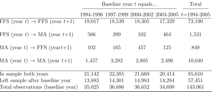
The need to calculate HCC scores in the pre-period means we generally limit our analysis to those individuals who were in FFS all twelve months of a baseline year, so that we observe their complete claims history that year. As such, much of the empirical strategy focuses on transitions from FFS to MA. Table 1 shows the number of observations who are in FFS in year t and in MA in year t+ 1, as well as the number who are in FFS both years (these individuals often serve as a control group), and how these numbers change across our sample period. We observe over 1,500 individuals who switch from FFS to MA, and over 70,000 who remain in FFS over the course of two years.
While relying on individuals who switch from FFS to MA is a limitation, it is not as serious as one might assume. Most individuals in MA have recently been in FFS, so these “switchers” are the norm, not the exception, in the MA population. The large share of switchers in the MA population can be seen in Table 1: 13 percent (1531÷(10,040 + 1531)) were in FFS the previous year. Moreover, we estimate that each year, over three-quarters of those joining MA are switching from FFS as opposed to joining MA as a new Medicare enrollee.19 Regardless, we address further potential biases arising from using the FFS-to-MA
flow as a proxy for the MA stock in the next two sections.
5 How did selection patterns into MA change after risk adjustment?
In this section, we empirically test the model’s predictions on selection patterns. As shown in the model, it is useful to decompose relative changes in total costs between MA and FFS
18See the online Data Appendix for further information. In practice, as we show in Appendix Table 3,
using the uncorrected MCBS capitation payment has minimal effects on our results. But given the problems we document in the Data Appendix, we think researchers should exercise caution when using this variable.
19During our sample period, approximately 2.2 percent of FFS recipients switch into MA in the following
year. With about 35 million in Medicare FFS during our sample period, roughly 770,000 (35,000,000*0.022) switch to MA per year. Each year during our study period approximately 2 million individuals become newly eligible for Medicare after turning 65 (ignore the 250,000 to 300,000 65-year olds who were already on Medicare because of Social Security Disability Insurance, who in general are less likely to join MA in any case). We see in the MCBS that about 11.7 percent of them are enrolled in MA in that first year, or roughly 234,000 (0.117*2,000,000). Thus, among the flow into MA each year, there is greater than a 3-to-1 ratio (770,000 to 234,000) of those who switch to FFS-to-MA versus those who join MA as soon as they become eligible for Medicare at 65.
enrollees after risk adjustment into a change in risk scores (“extensive-margin” selection) and a change in costs conditional on the risk score (“intensive-margin” selection). The model shows that, as plans are no longer incentivized to avoid enrollees with the conditions included in the risk formula, extensive-margin selection should fall, thus leading to an increase in risk scores among MA enrollees. The model also shows that intensive-margin selection should increase as plans now want to find enrollees who are “cheap” relative to their risk score; conditional on risk scores, total baseline Medicare expenditure for those switching to MA relative to those staying in FFS should fall after risk adjustment.
5.1 Quantifying the selection incentives created by the HCC model
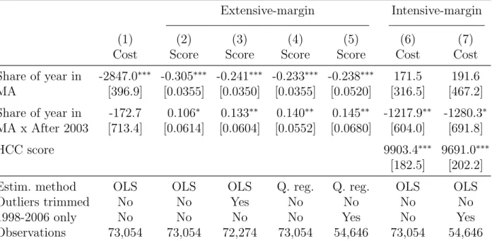
While Section 2 gave a general sense for how the HCC risk-adjustment model worked, it is useful to quantify the change in incentives before exploring whether plans reacted to them. Col. (1) of Table 2 presents the average difference between the HCC-based capitation payment and the traditional demographic-based capitation payment using our MCBS data, with this difference broken down by percentiles of the HCC score.20Mechanically, capitation payments must, on average, rise under the HCC formula for those with higher risk scores, and col. (1) merely presents the magnitudes. For example, the HCC capitation payment would, on average, pay $2,993 less than the demographic-based capitation payment for individuals with HCC scores in the lowest quartile, but it would pay more than $29,000 more for the individuals in the top one percent.
Col. (1) would make it seem as though plans would be incentivized to increase risk scores over the entire risk score distribution, but col. (2), which reports actual costs minus the HCC capitation payment, shows that doing so would not always be profitable on average. For example, individuals with the highest one percent of risk scores represent, on average, a nearly $6,000 loss to an MA plan, consistent with the work cited in Section 2 showing that HCC capitation payments for FFS enrollees with the most serious disease conditions would not fully cover these individuals’ FFS costs. Thus, increasing risk scores indiscriminately would lead plans to enroll some beneficiaries who would be highly unprofitable in expectation. While positive profits might still be possible if these individuals were very positively selected
20We estimate these payments using pre-2004 data on the population of individuals in FFS all twelve
months of the previous year, as we need full claims data to calculate risk scores for the following year. We use only the pre-period so that selection in reaction to the HCC model would not have already taken place. While this pre-period population might be selected because MA plans would have enrolled those most profitable under the demographic model, using data from 1994 alone, when MA penetration is under five percent, makes little difference. As described in the next Section, after 2003 MA plans enjoyed higher benchmarks as well as additional payments to ease the transition to risk adjustment, which we remove for the purposes of this table. As such, it reflects the change in incentives from “payment-neutral” risk adjustment as defined in Section 3.
along the intensive margin, these results suggest that plans might be reluctant to draw from the extreme right tail of the risk-score distribution.
Though not shown in the table, we also calculate that the share of individuals who are overpriced (have actual baseline costs less than their risk scores would predict) is 77 percent under both the demographic and the HCC model. Thus, risk adjustment does not actually decrease the number of individuals who are “over-priced”—though it obviously changes their likely characteristics—and indeed we find almost no change in MA market share after the HCC model is introduced.21 It is worth noting that extreme over-pricing is more common under the HCC model—more than twice as many individuals are over-priced by more than $9,000 under the HCC than under the demographic model.
5.2 Empirical strategy
The first element of the decomposition relates to whether plans, in response to risk adjust-ment, are less likely to avoid individuals with the conditions included in the risk formula. The prediction that such “extensive-margin” selection should fall suggests that we should see a relative increase in MA enrollees’ risk scores after 2003 and thus a positive coefficient on the interaction term in the following regression:
Risk scoreit =βM Ait×Af ter2003t+γM Ait+δt+it, (1)
whereiindexes the individual, t the year,Risk scoreit is the individual’s HCC score (which,
by definition, uses yeart−1 claims data to predict Medicare expenditure in yeart),M Ait the
share of her Medicare-eligible months that the individual spends in MA in yeart,Af ter2003 the post-period indicator, and δt a vector of year fixed effects.22 As will often be the case,
we estimate this regression on the sample of individuals who are in FFS all twelve months of the baseline year t−1 so that we can use their complete claims data that year to calculate year t risk scores.23 The model predicts a positive coefficient on the interaction term.
21Note that this analysis does not suggest that 77 percent of individuals are potentiallyprofitable before
and after 2003, as MA might be less efficient than FFS in providing the basic Medicare benefits package. The minimal change in MA market share before and after 2003 is the main reason we do not focus on whether MA or FFS is more efficient from a social-cost perspective. As we discussed in Section 3, the results of the model go through whether MA or FFS is more efficient so long as risk-adjustment does not induce large changes in MA market share.
22Both equations (1) and (2) are parsimonious in that they do not control for demographic or other
characteristics of the beneficiaries. This choice is deliberate, and it reflects the fact that MA plans are paid based on the risk scores of their beneficiaries, not their risk scores conditional on, say, age.
23While we could potentially use the administrative risk scores provided by CMS for the post-period,
throughout this section we use our simulated risk scores in both the pre- and post-periods so that any change in risk scores between the two periods cannot be driven by differences in how they are calculated. Using the actual risk scores in the post-period increases the magnitudes and statistical significance of the coefficients of interest in both the extensive- and intensive-margin analyses. As our simulated risk scores likely
The second element of the decomposition relates to the “intensive-margin” prediction that after risk adjustment, plans will enroll individuals who have low baseline costs conditional on their risk score because they are more positively selected along dimensions excluded from the formula. As such, we predict a negative coefficient on the interaction term of the following regression:
Expenditurei,t−1 =βM Ait×Af ter2003t+γM Ait+λRisk scoreit+δt+it, (2)
where Expenditurei,t−1 is the total FFS expenditure for individual i in year t−1 and all
other notation and sampling follows that in equation (1).24
5.3 Results
We begin by exploring how the difference in total baseline costs change after risk adjustment among those switching to MA versus those remaining in FFS, and then decompose this effect into its extensive- and intensive-margin components. Col. (1) of Table 3 shows that before risk adjustment, those switching to MA have baseline costs $2,847 below those who remain in FFS, consistent with past work cited earlier on the substantial positive selection into MA. Risk adjustment has no apparent effect on this selection (in fact, the point-estimate, -$173, suggests it may have increased). Thus, while the goal of risk adjustment was to end plans’ incentives to cream-skim low-cost enrollees, we find no evidence that those joining MA after 2003 have higher costs.
The next three columns of Table 3 explore the first component of the decomposition—the change in the risk score. Col. (2) suggests that while individuals switching into MA before risk adjustment had risk scores roughly 0.31 points lower than those remaining in FFS, risk scores of those switching into MA rise after risk adjustment is introduced, making up about a third of the difference.
Based on the results from Table 2 that extreme outliers in the right-tail are still under-priced by the HCC formula, we expect the effect on the mean to be muted, as plans would still be wary of enrolling those with extreme risk scores. Indeed, in col. (3), merely dropping observations with risk scores above the 99thpercentile substantially increases the magnitude of the estimate. Estimating a median regression (col. 4) on the entire sample increases the coefficient by nearly a third, so that sixty percent of the pre-period gap in risk scores between have some measurement error, we attribute this difference to less attenuation bias when the administrative risk scores are used in the post-period.
24This specification is similar in spirit to the “unused observables” test of Finkelstein and Poterba (2006).
Using the terminology of their framework, Expenditurei,t−1 in equation (2) is an “unused observable”
because it is positively related to future costs to the insurer but, conditional on a beneficiary’s risk score, is not used to determine insurance premiums or capitation payments.
FFS and MA is made up by the increase in MA risk scores after risk adjustment. While we generally prefer to use a long pre-period in order to improve precision by increasing the number of individuals switching from FFS to MA, col. (5) shows that excluding observations before 1997 does not change the results. As shown in Appendix Table 3, the results are robust to using a dummy variable for MA status instead of the share of the year an enrollee is in MA.25
Following Bitler et al. (2006), to get a clearer picture of the change across the entire distribution we estimate quantile regressions for the first through 99th quantiles, and plot the resulting coefficients in Figure 2. As predicted, the effect is especially strong for higher quantiles (due to the greater variance at higher risk scores, these individuals are very at-tractive after risk adjustment due to the greater scope for intensive-margin selection). But it falls close to zero right before the 99th quantile, consistent with outliers being substantially
underpriced by the formula.
Given that total costs of those switching to MA relative to those remaining in FFS do not change after 2003 while their risk scores rise, then, mechanically, intensive-margin selection must have increased and the remaining columns of Table 3 merely quantify this effect. Col. (6) shows that, relative to the pre-risk-adjustment period, after 2003 individuals switching into MA versus those remaining in FFS have baseline costs over $1,200 less than their risk scores would predict. As with the extensive-margin results, the coefficients of interest are robust to excluding years before 1997 (col. 7) and using a dummy-variable for MA status (see Appendix Table 3).26
Interestingly, in its 2012 annual report to Congress, MedPAC, citing a working-paper version of our study, found nearly identical levels of intensive-margin selection levels using the universe of Medicare enrollees in 2007 and 2008.27
25We also tested whether using a long pre-period was biasing the results by including a trend estimated
using the pre-period data. The coefficient on the variable F raction of year in M A×year is if anything negative, but is indistinguishable from zero (p=0.886). Not surprisingly, when it is included in the main regressions, the coefficient of interests increase slightly (from, for example, 0.133 in col. (2) of Table 3 to 0.155). If we break up the post-period into separate years, the coefficients, though noisy, show a monotonic increase in extensive margin selection over the post-period. The results in the table are also robust to excluding those from institutions.
26We also perform the same analysis that was described in footnote 25. The coefficient on the pre-period
trend is slightly negative but essentially zero (p= 0.89). Including it in the main regression slightly reduces the magnitude of the coefficient of interest (from -1217 in col. (6) of Table 3 to -1052), but it remains statistically significant. Like the extensive-margin results, the magnitude of the effect increases over the post-period years, though there is some slippage in 2005. The results are also robust to dropping those living in institutions.
27See www.medpac.gov/documents/Jun12_EntireReport.pdf, pp. 101. MedPAC finds that “the [MA]
joiners [those in FFS in 2007 and MA in 2008] had costs that were 15 percent lower than the stayers [those in FFS both years].” This effect is almost identical to our estimates of intensive-margin selection in the post-period. In the main intensive-margin specification (col. 6 of Table 3), the coefficient on theM A main effect is 171.5 and that onM A×Af ter is -1217.9, for a total effect of -1046.4 (171.5-1217.9). Average costs
5.4 Discussion and further verification
One of the central drawbacks of our identification strategy is that, because we must calculate risk scores using FFS claims data, we must sample individuals who are in FFS in a baseline year and identify our coefficients off of those who switch the following year from FFS to MA. While we have shown that such switchers are more common than those who enroll at 65, we also provide additional evidence that supports the results of this “switcher” analysis but that uses data on all those in MA or FFS in a given year (regardless of where they were the previous year).
As noted earlier, CMS provided us with actual risk scores for all individuals in the MCBS—whether in FFS or MA, “switcher” or “stayer”—from 2004 to 2006. Given the lack of pre-data, we cannot replicate the specification in Table 3, but we can determine whether risk scores among MA enrollees are growing faster than those in FFS during this period, as one might expect both because risk adjustment phases in during this period and because MA plans’ ability to enroll individuals with high risk scores may improve over time. Indeed, in the CMS administrative data, MA risk scores increased by 12 percent over this three-year period, while FFS risk scores increased by one percent, resulting in an MA-FFS difference in average risk scores of -0.13, -0.11, and -0.045 in 2004, 2005 and 2006, respectively. Though far noisier, when we estimate year-by-year post-period effects using our sample in Table 3, we also find a monotonically increasing pattern with much of the gain between 2005 and 2006 (the corresponding differences are -0.18, -0.17, -0.08). As such, at least along this measure, our estimates comparing those who switch to MA to those who remain in FFS closely correspond to comparisons using the stock of individuals in MA versus FFS.28
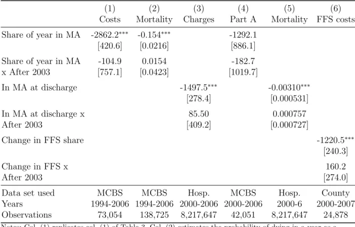
While much of the analysis in this section requires knowing the risk score, the first result—that those switching to MA are just as positively selected on total baseline costs after risk adjustment as before—does not, and as such we can use data that does not include risk scores to verify this unconditional spending result. Table 4 takes up this task, with col. (1) replicating the original result from Table 3. We begin by using mortality as a proxy for health costs and because we have this information for everyone in the MCBS, we no longer for FFS stayers in the post risk adjustment period are 7435.3. Thus, the MA joiners are on average 14.1 percent (-1046.4/7435.3) cheaper than the FFS stayers in 2004-2006, very close to MedPAC’s estimates. In fact, they find evidence of intensive-margin selection in 68 of the 70 HCC categories, a result that, given the relatively small sample size in the MCBS, we cannot credibly investigate ourselves. In other words, MedPAC finds that, on average, beneficiaries who enroll in MA have significantly lower costs than those on who remain on FFS even controlling for the risk score and looking within specific HCC categories. It is reassuring to know that the effects we estimate through 2006 remain in 2007 and 2008 in a much larger sample.
28Readers may note that the regression estimates in Table 3 there is still a substantial difference in FFS
and MA risk-scores, whereas the evidence from CMS suggests that MA risk scores essentially “caught up” to those of FFS by 2006. The faster catch-up among the MA stock than among those switching from FFS is likely due to intensive coding, which does not affect individuals who were in FFS the previous year.
need to rely on switchers. Mortality is a powerful proxy for total costs. As noted earlier, the HCC formula explains 11 percent of the variation in FSS spending; a dummy variable for dying in a calendar year explains by itself 14 percent. The assumption is that if plans are indeed enrolling higher-cost individuals, we should see an increase in relative mortality rates among MA enrollees. Col. (2) of Table 4 shows that there is no relative change in mortality rates among those in MA after 2003—while the point-estimate on the interaction term is positive, it is essentially zero with a p-value of 0.714 despite a sample of nearly 140,000 (19,000 of which are in MA).
We also move beyond the MCBS to verify these results. We gathered over 8,000,000 hos-pital discharge records from the twelve states between 2000 and 2006 that require hoshos-pitals to record FFS/MA status. Because these states are populous, the state-years in our data represent 42 percent of Medicare beneficiaries during this period. In col. (3), the average MA patient had $1,500 less in charges than his FFS counterpart before 2004—consistent with positive selection in the pre-period—with only $85 (p=.835) of this difference being made up in the post-period—consistent with our results that risk adjustment did not lead MA plans to enroll higher-cost individuals. Interestingly, when we do our best to replicate this regression with the MCBS switcher-analysis by using only Part A charges in 2000 to 2006, we find very similar point-estimates (col. 4).29 Col. (5) shows that the hospital discharge data show very similar (null) results on relative mortality changes among MA patients after 2003.
Finally, we follow Batata (2004) and use county-level data to estimate changes in MA se-lection. She shows that regressing county-level changes in average FFS costs on the change in county-level MA penetration yields a measure of the difference in costs between the marginal person switching between MA and FFS and the FFS stock. While slightly different than our switcher regressions—which compare the average person switching from FFS to MA with the average person staying in FFS—one would expect these two selection measures to move in the same direction. As the final column of Table 4 shows, this difference is negative before risk adjustment, reflecting the fact that those on the margin of switching between MA and FFS have lower costs than those in FFS, and, consistent with the switcher analysis and the rest of the table, does not change after risk adjustment.
In summary, evidence from a wide variety of datasets shows that, with respect to overall
29An important difference between the MCBS part A results and the hospital discharge results is that the
former is aggregated across the entire year for an individual, whereas the latter is a per-episode measure. However, the share of hospital episodes accounted for by MA enrollees increased at a slightly slower (though essentially equal) rate after 2003 than did the total MA share of Medicare enrollees in these states, meaning that there is neither an increase in the per-visit cost for MA enrollees relative to FFS enrollees after 2003 nor in the average number of hospital visits per year.
average costs, those in MA are just as positively selected after risk adjustment as they were before. This null result is explained by two significant, offsetting changes—an increase in risk scores and a simultaneous decrease in costs conditional on the risk score—both of which were predicted by the model. However, our model cannot predicta priori whether these offsetting changes are enough to completely “un-do” risk adjustment with respect to the government’s goal of reducing differential payments.
6 Did risk adjustment decrease differential payments to MA plans?
In this section, we focus on how an individual’s annual Total Medicare expenditure changes as he switches from FFS to MA. Recall from Section 4 that Total Medicare expenditure is equal to the total cost to Medicare for an individual, whether it is covering her directly via FFS or paying an MA plan to cover her. If risk adjustment works perfectly—so that in expectation capitation payments are equal to an individual’s FFS costs—then whether an enrollee switches between FFS and MA should have no effect on his total Medicare expenditure levels.
Before exploring how differential payments changed after 2003, we begin by testing the model’s prediction that risk adjustment would have “worked”—reduced differential payments—had selection patterns not changed. To test this claim, we focus on enrollees who switched from FFS to MA in the pre-period, when selection with respect to the HCC formula would not yet have taken place. We find that capitation payments—and thus differ-ential payments—would have decreased by $734 dollars, on average, had the HCC formula and not the demographic formula been used on this sample. Of course, as shown in the pre-vious section, the characteristics of those joining MA change in response to risk adjustment, and the rest of the section explores how differential payments change as a result.
6.1 Empirical strategy
To isolate the effect of the introduction of risk adjustment from other changes occurring around the same time, we make two adjustments to capitation payments after 2003. First, the growth rate of county benchmarks (the baseline value, which, multiplied by the risk score, yields capitation payments) began to rise more rapidly in the later years of our sample period. We thus calculate each county’s benchmark growth rate in the pre-period and then have the county’s benchmarks grow at this slower rate for the post-period as well. Second, in the years immediately following the introduction of risk adjustment, plans received so-called “budget-neutrality” adjustments (about a ten percent increase in the risk-adjusted portion of capitation payments) to ease the transition to risk adjustment, and we mechanically reduce
payments to remove this effect. In both cases, these adjustments increased all capitation payments by a given percent and did not depend on underlying individual conditions or characteristics. The adjustments we make obviously decrease the likelihood we would observe an increase in differential payments after risk adjustment.
We begin, as before, with the sample of beneficiaries in FFS all twelve months of a given year t−1. To estimate the counterfactual Medicare expenditure for an MA joiner in year t had he remained in FFS, we examine the actual Medicare costs in year t for FFS stayers who are similar along observable dimensions. The estimating equation is:
Expenditureit =βM Ait×Af ter2003t+γM Ait+λXit+δt+f(Expenditurei,t−1) +it, (3)
whereExpenditureitis total Medicare expenditure for personiin yeart,f(Expenditurei,t−1)
is a flexible function of lagged Medicare expenditure, and all other notation follows that in previous equations.30Note that in the intensive-margin regression we modeled an individual’s Medicare expenditure the year before joining MA—hypothesizing that individuals who have low baseline FFS spending conditional on their risk score would be highly attractive to MA plans after risk adjustment—whereas here we model current Medicare expenditure. While lagged Medicare expenditure is highly correlated with current Medicare expenditure and thus serves as an obvious factor on which plans would try to screen, it is the current expenditure that an MA plan must actually cover once someone has joined and thus current expenditure is what matters for estimating differential payments.
This regression model (as well as the ones in the previous section) estimate how charac-teristics of those switching to MA change after risk adjustment and do not take into account that the quantity of individuals in MA might change as well. As depicted in Appendix Figure 1, the MA share of the Medicare population increases in the post-period (as does the proba-bility of switching from FFS to MA), so our ignoring the quantity margin would understate the effect of any differential payment increases as they would apply to a larger number of MA enrollees in the post-period.
6.2 Results
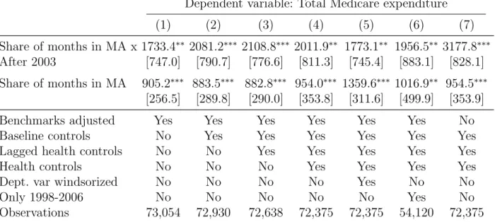
The first column of Table 5 shows the results from regressing the level of total Medicare spending on the MA variable, which is allowed to have a different effect before and after risk
30We prefer this specification to simply regressing ∆Expenditure
it as the lagged expenditure controls in
equation (3) can better account for the fact that medical costs typically exhibit strong regression to the mean, though results using ∆Expenditureit look very similar and are reported in Appendix Table 3. The
lagged Medicare expenditure controls include: lagged Part A and B expenditure and deciles of non-zero Part A payments and non-zero Part B payments as well as indicator variables for zero Part A and B payments (we found that regression to the mean differed depending on the type and level of costs). The results are not sensitive to controlling more coarsely or finely than deciles for lagged Part A and B expenditure.
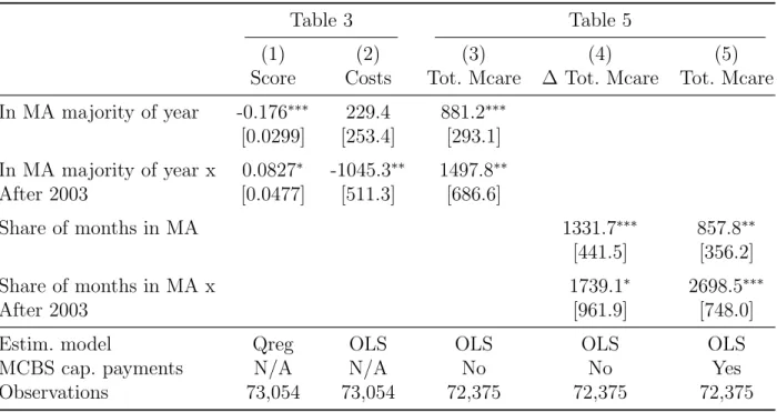
adjustment, the lagged spending variables, and year fixed effects. Total Medicare expenditure increases by roughly $905 when an individual switches from FFS to MA (for the entire year) before risk adjustment, and by an additional $1,733 after risk adjustment.
The second column adds county fixed effects as well as demographic and other basic controls (all listed in the table notes). The coefficient on the interaction term increases to $2,081. These controls are important if, for example, older people tend to have higher spending growth and post risk adjustment they are also more likely to join MA plans. In this case, we want to account for the fact that these older beneficiaries would have likely experienced high cost growth had they remained in FFS. Col. (3) includes measures of lagged health indicators, which has essentially no effect on the coefficient on the interaction term. Col. (4) includes health indicators from the current year. While self-reported health is not a perfect proxy for current-year health costs, this specification better accounts for potential regression to the mean in health status—if enrollees typically experience a deterioration in their health upon joining MA, then comparing current to previous year’s spending will over-state MA differential payments; however, current-year health status is endogenous to the care individuals receive in MA versus FFS and thus including it may be “over-controlling.” In practice, the two estimates are very similar.31
Cols. (5) and (6) subject the estimation in col. (4) to robustness checks. Windsorizing the data based on the 99th percentile in col. (5) or dropping years before 1998 in col. (6) leave the results largely unchanged. Appendix Table 3 shows the results are robust to mea-suring MA status with a dummy variable and using changes in M edicareExpenditure as the dependent variable instead of levels with lagged explanatory variables. Appendix Table 4 replicates all of Table 5, but uses our simulated HCC scores to calculate post-period capi-tation payments instead of the administrative HCC scores from CMS. The point estimates are almost identical.32
31We explore whether individuals tend to join MA just as their health is about to deteriorate or as their
spending is about to rise for other reasons, which would cause us to underestimate the costs MA plans actually face and thus to overestimate overpayments. First, if this effect were important, we should have seen a large decrease in β and γ after current health measures were added in col. (4). Second, individuals are unlikely to postpone expensive treatments until they join an MA plan because plans tend to have less generous cost-sharing for serious procedures than does FFS (see Kaiser’s report on MA benefits, http:
//www.kff.org/medicare/upload/8047.pdf). Third, we actually find no evidence of strategic timing of
services for which MA is more generous than FFS, such as vision exams. Finally, we find no evidence of an “Ashenfelter dip” the year before a switch to MA—controlling for two years of lagged cost data instead of one has minimal effect on the point-estimates, though standard errors increase due to the smaller sample.
32As with the selection results, we explore whether there are any pre-trends in the data. The coefficient
on the MA trend is close to zero (p = 0.7). Controlling for the trend reduces the point-estimate on the col. (4) specification to $1482, though it remains statistically significant. As with the selection results, the year-by-year point estimates in the post-period are noisy, but exhibit a positive trend (though, like the intensive-margin results, the trend is not monotonic, with slippage in 2005). The results are also robust to excluding individuals living in institutions.