Developing object detection, tracking and image mosaicing algorithms for visual surveillance

(1)

Developing Object Detection, Tracking

and Image Mosaicing Algorithms for

Visual Surveillance

by

Taygun Keke¸c

Submitted to the Graduate School of Sabancı University in partial fulfillment of the requirements for the degree of

Master of Science

Sabancı University August, 2013

(2)

(3)

c

(4)

Developing Object Detection, Tracking and Image Mosaicing

Algorithms for Visual Surveillance

Taygun Keke¸c ME, Master’s Thesis, 2013

Thesis Supervisor: Prof. Dr. Mustafa ¨Unel

Keywords: Detection, Tracking, Background Subtraction, Image Registration, Stitching and Mosaicing

Abstract

Visual surveillance systems are becoming increasingly important in the last decades due to proliferation of cameras. These systems have been widely used in scientific, commercial and end-user applications where they can store, extract and infer huge amount of information automatically without human help.

In this thesis, we focus on developing object detection, tracking and image mosaicing algorithms for a visual surveillance system. First, we review some real-time object detection algorithms that exploit motion cue and enhance one of them that is suitable for use in dynamic scenes. This algorithm adopts a nonparametric probabilistic model over the whole image and exploits pixel adjacencies to detect foreground regions under even small baseline motion. Then we develop a multiple object tracking algorithm which utilizes this algorithm as its detection step. The algorithm analyzes multiple object in-teractions in a probabilistic framework using virtual shells to track objects in case of severe occlusions. The final part of the thesis is devoted to an image mosaicing algorithm that stitches ordered images to create a large and visually attractive mosaic for large sequence of images. The proposed mosaicing method eliminates nonlinear optimization techniques with the ca-pability of real-time operation on large datasets. Experimental results show that developed algorithms work quite successfully in dynamic and cluttered environments with real-time performance.

(5)

G¨

orsel G¨

ozetim i¸cin Obje Tespiti, Takibi ve G¨

or¨

unt¨

u

Mozaikleme Algoritmalarının Geli¸stirilmesi

Taygun Keke¸c ME, Master Tezi, 2013

Tez Danı¸smanı: Prof. Dr. Mustafa ¨Unel

Anahtar Kelimeler: Obje Tespit, Takip, Arkaplan Ç ıkarma, Görüntü Kayıt, Dikme ve Mozaikleme

¨ Ozet

Son yıllarda kameraların ucuzlamasıyla g¨orsel g¨ozetleme sistemlerinin ¨

onemi gitgide artmaktadır. Bilimsel, ticari ve son kullanıcı uygulamalarında yaygın olarak kullanılan bu sistemler yo˘gun miktarda bilgiyi depolayabilir, ayıklayabilir, ve bu bilgileri bir insanın yardımı olmadan yeni bilgi ¸cıkarımında kullanabilir.

Bu tezde, bir görsel gözetim sistemi kapsamında kullanılabilecek obje tespit, takip ve görüntü mozaikleme algoritmalarının geli¸stirilmesine yo˘ gunla-¸sılmı¸stır. ˙Ilk olarak ger¸cek zamanlı ¸calı¸sabilen, hareket ipu¸clarını kullanan obje tespit algoritmaları incelenmi¸s ve dinamik sahnelerde de ¸calı¸sabilecek bir obje tespit algoritması geli¸stirilmi¸stir. Adı ge¸cen algoritma, nonparametrik olasılıksal bir model aracılı˘gı ile piksel kom¸suluklarını kullanarak görüntüdeki ¨

onplan bölgelerini ufak kamera hareketleri altında tespit edebilmektedir. Bun-dan sonra, önerilen obje tespiti algoritmasını bir önadım olarak kullanan bir ¸coklu obje takibi yöntemi geli¸stirilmi¸stir. Algoritma ¸coklu obje etk-ile¸simlerini olasılıksal bir ¸cer¸cevede inceleyerek, sanal kabuklar ile yo˘gun ¨

ortmeye sahip durumlarda objeleri takip etmektedir. Tezin son bölümünde ise sıralı görüntüleri dikerek daha geni¸s ve görsel olarak etkileyici bir mozaik olu¸sturan bir görüntü mozaikleme algoritması önerilmi¸stir. Önerilen yöntem lineer olmayan eniyileme tekniklerini devre dı¸sı bırakarak, geni¸s görüntü kümeleri i¸cin dahi ger¸cek-zamanlı ¸calı¸sabilmektedir. Deney sonu¸cları g¨ oster-mektedir ki, önerilen algoritmalar ger¸cek zamanlı olarak dinamik ve kalabalık ortamlarda ba¸sarıyla ¸calı¸smaktadır.

(6)

Acknowledgements

It is a great pleasure to extend my gratitude to my thesis advisor Prof. Dr. Mustafa Unel, who has taught me patience and contemplation, for his precious guidance and support. I am indebted to him for his supervision and excellent advises throughout my Master study.

I would gratefully thank Assoc. Prof. Dr. Hakan Erdogan for his support through my studies.

Finally, I would like to thank my mother who I can not pay back her efforts for my studies, and to my colleagues Barı¸s Can Üstünda˘g, Alper Yıldırım, Mehmet Ali Güney, Soner Ulun, Sanem Evren, and my friends Mehmet Fatih Do˘gan, Salih Yıldırım, Sümeyra Balcı, Sinem Karacabey and Esra Nur Varlı who supported me throughout my studies.

(7)

List of Figures

1.1 Estimated billion dollar market of video surveillance in 2012-2020 [1]. . . 5 2.1 A 2D GMM model having 3 different mixtures each having

different mean and variance . . . 11 2.2 Rows correspond to original image and results of Adaptive

Median, Prati Median and EigenBackground algorithms on car scene. . . 16 2.3 Rows correspond to original image Grimson GMM, Zivkovic

GMM and Wren GMM algorithms respectively on car scene. . 17 2.4 Precision and recall values of the experiments. . . 18 2.5 Result of GMM algorithm on Camera1 sequence obtained from

PETS200 database. . . 20 2.6 Some scenes having dynamic pixels like tree leaves, flowing

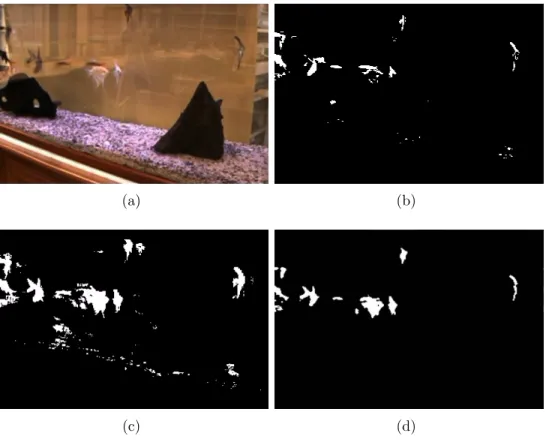
water and shiny aquarium pebbles. . . 21 2.7 a) An image from aquarium dataset b) Adaptive-Median based

background subtraction result c) GMM based background sub-traction result d) Proposed background subsub-traction result. . . 26 2.8 a) Two image from aquarium dataset b) Result of Background

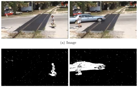
and Foreground Modeling c) 3x3 Weighted Median Filter as last step d) 5x5 Weighted Median Filter as last step . . . 27 2.9 a) Two image from railroad dataset b) Result of Background

and Foreground Modeling c) 3x3 Weighted Median Filter as last step d) 5x5 Weighted Median Filter as last step . . . 28

(10)

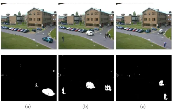
2.10 a) Two image from PETS dataset b) Result of Background and Foreground Modeling c) 3x3 Weighted Median Filter as last step d) 5x5 Weighted Median Filter as last step . . . 29 3.1 a)An object Oi with its minimum shell Sb and instantaneous

shell Sr is depicted. b) Shells dynamically grow and shrink

with time. . . 34 3.2 a) State transitions of object to object relations. b) State

graph where thin edges represent INTERACTION and thick edges represent JOINT relationship between objects. . . 35 3.3 Demonstration of Case IV (green and red) and Case V (purple

and orange). . . 37 3.4 a) Aquarium image b) Background subtraction c) Output of

the event resolution and pixel membership evaluation where pixels of each object are colored differently for illustration pur-poses . . . 39 3.5 Our experimental setup: aquarium environment. . . 44 3.6 Sequence from PETS database. . . 45 3.7 Tracking accuracy for PETS Sequence where each color

rep-resents a tracked object. . . 46 3.8 Sequence from Caviar database . . . 47 3.9 A tracking sequence from aquarium where three fish interact . 48 3.10 A tracking sequence from aquarium where several fish interact 49 4.1 Flowchart of our mosaicing approach. . . 56

(11)

4.2 Drift caused by estimation errors. UAV returns to same area and snaps same image from initial position. True and esti-mated trajectories are shown with green and red dashed curves respectively. . . 57 4.3 Comparison of pairwise stitching using Equation 1 and

stitch-ing usstitch-ing cost function 3 (bottom). Note that misregistrations caused by error in the leftmost frames are prevented in the sec-ond case. . . 59 4.4 An illustration of SAT. For a selected projection axis Pk,

pro-jected convex sets did not intersect. Dashed green line is an example separator for this projection axis. . . 64 4.5 Czyste sequence. Images represent before and after blending

respectively. . . 69 4.6 Final aerial mosaic constructed from Munich Quarry sequence 70 4.7 Final aerial mosaic constructed from Eastern Island sequence . 70

(12)

Chapter 1

1

Introduction

This thesis addresses the problem of developing robust object detection, tracking and mosaicing algorithms in the context of visual surveillance. Vi-sual surveillance systems employ these algorithms as submodules. Neverthe-less, these algorithms have diverse application areas and can also be utilized in different contexts. We focus on obtaining effective solutions to aforemen-tioned problems under real time constraints.

Surveillance is monitoring behavior, activities, or other changing informa-tion, usually of people for the purpose of managing, directing, or protecting. Surveillance systems are technological tools to increase perception and situa-tional awareness [2]. These automated systems help decision making process of humans with their analysis of events in the scene. As humans, we do not have ability to gather and store high quantity of information. Instead, surveillance systems can gather gigantic quantity of data and process it in which humans cannot perform easily. In literature, there have been different modalities for surveillance systems [3, 4].

There have been surveillance systems based on chemical, sound and vi-sual sensors [5]. Out of all these systems, vivi-sual surveillance has proved to be most useful due to proliferation of video cameras and recent advancements in computer vision techniques. With our current technology, the concept of

(13)

visual surveillance is mostly implemented using CCD cameras. The ultimate goal of these visual surveillance systems is to extract meaningful information from acquired dense image data. To achieve this purpose, a visual surveil-lance system consists of several modules such as object detection, tracking and recognition [6]. Detection and tracking algorithms facilitate automatic detection of targets and tracking their behaviour without any human inter-vention.

Automatic object detection is an attempt to scene understanding and video analysis. It is an essential step to make inference about the scene. These methods can infer number of objects and existence of specific objects in that scene. The methods can exploit object motion [7], appearance [8] or both. These algorithms may be run on each acquired frame, or until a tracking procedure is initialized.

Object tracking is quite popular in many applications. There have been extensive studies on the topic [9]. In literature, much research has been done using point [10], kernel [11] and curve tracking [12]. Many high level appli-cations contain an object tracking procedure. The methods have different object and motion representations based on the application scenario. Apart from selection of appropriate image features and motion models, many of these algorithms require an object detection routine.

Image mosaicing algorithms extend field of view of surveillance system to a much larger scope [13]. The mosaiced image, having a larger field of view, can provide more information than spatially and temporally distinct separate images. These algorithms can be used to stabilize motion or enlarge field of view of a moving camera. In what follows, we focus on finding efficient solutions to these three problems.

(14)

1.1

Motivation

The problems of object detection, tracking and image mosaicing have cap-tured the interest of both the research and industrial communities in the last decade. These algorithms have such a large applicability that they are com-monly used in many different contexts. Surveillance based application areas contain safety in transport applications [14, 15], monitoring of railway sta-tions [16, 17], urban and city roads [18, 19], navigation, tourism and military [20]. Apart from surveillance context, they are also commonly used in fields of medical imagery [21]. The automated systems utilizing these algorithms have noticeably higher response time than human operated systems. Main advantages for using vision based solutions to these problems can be listed as follows:

• They require inexpensive equipment such as a CCD camera and an inexpensive computer.

• They provide high rate data (generally 25-30hz). The upper limit of processing is determined by the power of computing environment.

• The acquisition is passive and more secure unlike other methodologies such as LIDAR.

• Position estimation is also possible without extra sensors.

• Power consumption is lower compared to other sensors.

Nevertheless, the biggest two disadvantages of such vision systems are:

• High vulnerability to visibility conditions such as weather conditions, clouds and other external disturbances.

(15)

• Many vision based algorithms require enough visual cues to be found which may not be possible for some scenarios.

In light of these facts, vision based solutions are highly seductive for at-tacking detection and tracking problems. The systems performing these tasks automatically are becoming more and more popular [2]. The main reason is that even well trained personnel cannot maintain their attention for extended periods of time. They suffer degradation of performance after several hours. Another requirement for such systems is the economical reasons, namely the need for lowering costs. Humans can not maintain multiple tasks simultane-ously, one must hire dozens of personal to perform surveillance on multiple or large areas. This increases personal expenses significantly. Moreover, hu-man operator’s response time is much slower than automated solutions. All these factors encourage automation of surveillance using robust and effective computer vision algorithms.

These observations are further validated with growing market of auto-mated surveillance. By the year 2012, total revenue in autoauto-mated surveil-lance market reached $13.5 billion. Revenue by the year of 2020 is estimated to reach $39 billion [1]. The estimated market revenue is shown on Figure 1.1. By year 2011, over 165 million video surveillance cameras installed worldwide captured 1.4 trillion video-hours. Captured video surveillance will reach ap-proximately 3.3 Trillion video-hours in 2020. Deployment of video cameras is so rapidly increasing that even small shops adopt cheap CCTV cameras for security purposes. The market analysis and latest reports about the vi-sual surveillance field concludes that the growth of the field will continue to accelerate.

(16)

Figure 1.1: Estimated billion dollar market of video surveillance in 2012-2020 [1].

1.2

Thesis Organization and Contributions

The purpose of this thesis is to develop effective object detection, tracking and image mosaicing algorithms that can not only be used in surveillance but also in different contexts. In Chapter 2 we first compare some State of the Art object detection methods which are based on background subtraction, and develop an object detection algorithm which can cope with dynamic scenes and robust to camera jitter while being able to operate in real-time speed. The experimental results for proposed method is shown on aquarium setup.

In Chapter 3, we propose a multiple object tracking algorithm that han-dles object interactions and solves data association problem effectively. The proposed method uses object detection algorithm proposed in Chapter 2 for detecting region of interests in the scene. The tracking results have been shown on aquarium setup and various publicly available datasets.

(17)

The method uses ordered aerial images captured from a camera under Eu-clidian motion and capable of creating consistent large scale mosaics in real-time. The novelty of the proposed algorithm lies on avoiding nonlinear min-imization while sustaining real-time capability even on large scale data. The experimental results are shown on images captured from an UAV.

Chapter 5 concludes the work done in this thesis and indicates possible future directions.

(18)

Chapter II

2

Object Detection with Background

Subtrac-tion

Object detection is the process of locating objects in the scene. The methods for detecting objects can be classified into two groups. First group consists of appearance based detection methods [22]. In these methods some visual features from a dictionary is searched in the image. When a viable set of matches is found, an object is meant to be detected [23]. A second group of methods are motion based detection methods [24]. These methods, also called as motion segmentation or background subtraction, exploit motion in the scene to detect abnormalities. The problem can be described as follows: determine each pixel label as foreground or background. Main difficulties of background subtraction are camera jitter, momentary illumination and low quality images due to cheap visual sensors. Moreover, movement of scene objects, new objects added to the scene, object shadows are challenges need to be faced for developing a robust approach. A robust approach must consider all these difficulties under memory and speed constraints [25].

First background subtraction methods were based on creating a subtrac-tion image between consequent images using a binary thresholding mech-anism to obtain pixel labels. These methods were fast but not so robust on challenging scenarios and were very sensitive on selected threshold value.

(19)

There have been some methods that propose to store a windows of pixel history in time domain and obtain a representative profile of each pixel to belong to the background. The thresholding was carried out after profiling step. Nevertheless, real-time scenes required more advanced methods. The pioneering work in the field has been done by Grimson and Stauffer [26]. They proposed GMM (Gaussian Mixture Model) based background subtrac-tion technique. In the cited work, each pixel was modeled with a number of Gaussian distributions each having different mean and variances. The pixel profile were updated with new incoming pixel values. This probabilistic in-troduction yielded nice results. Apart from GMM based subtraction, Oliver et al. proposed using Eigen-Space approach [27] for noise-free background subtraction. The whole background image vector was created using a number of learned frames (as samples). Then the vector was averaged and a mean image is formed which is the model for background image.

As the statistical methods rise into power, Kernel Density Estimation based background subtraction approaches become popular [28, 29]. These methods were modeling both background and foreground using a density es-timation. They utilize a kernel function (mostly Gaussian or Epanechnikov) to represent data. The most problematic thing with these approaches were memory requirement due to non-discarded data. After background learning phase, collected bandwidth of data represents a nonparametric probability distribution.

2.1

Real-Time Background Subtraction Algorithms

In this section, accuracies of several background subtraction algorithms for object detection purposes are evaluated. The selected algorithms have

(20)

real-time capabilities. They are learning based where a number of frames must be fed into the learning system in order to learn the background model. After the learning phase, all algorithms create their background model (or background image). The final thresholding is then applied for obtaining pixel classes as foreground or background.

First class of algorithms in this comparison is Median based subtraction algorithms. These algorithms are powerful in the sense that they can cope with arbitrary noise which may be caused by camera jitter or sensor defi-ciencies. A commonly used algorithm in this class is Adaptive Median [30], which is the fastest and simplest subtraction algorithm in this comparison. After learning a number of sample frames, algorithm computes the median intensity of each pixel in the scene. Using this intensity profile, forthcoming values pixels are evaluated. For each pixel, a history is kept, sorted and median value of the history is updated within a sliding window of frames. Forthcoming pixel value is thresholded to determine whether it is coherent with the background model of that individual pixel, represented with its median.

Another variant of Median based subtraction is proposed by Prati et. al [31]. In the cited work they used a different median function as follows:

Bt+∆t(p) = arg min ˆ_i k X j=1 D(xi, xj), xi, xj ∈S (1)

where Bt+∆t(p) is the background model of a pixel at time t+ ∆t, D is the distance function, xi and xj are elements of that pixel model respectively

and S is the set containing pixel history of background model. The selected minimum argument represents the color model of the pixel. While one can

(21)

use different distance functions, L∞ distance is chosen in the cited paper:

D(xi, xj) = arg max

ˆ

c |xi,c−xj,c| (2)

where c denotes selected color in RGB color space. These median based algorithms are computationally more efficient than GMM based subtractions. However, they must be selected only in very limited computing environments in which speed has more importance than detection accuracy.

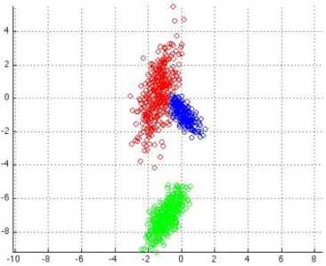
Another family of detection algorithms are Gaussian Mixture Model (GMM), also called Mixture of Gaussians (MOG), based algorithms. These algorithms have found to be very successful in many scenarios. The first work in this family has been proposed by Stauffer and Grimson [26]. In this approach, each pixel is represented by K different 1D Gaussian probability densities having distinctive mean and variance (Fig 2.1). Each gaussian density has different weights. In many GMM based algorithm, the covariance matrix is assumed to be diagonal for computational reasons. Given mixture model, probability of a pixel X at time t to belong to the background can be given as:

P(Xt) = K

X

i=1

wi,t η(Xt, µi,t,Σi,t) (3)

where P(Xt) is the probability of a pixel X at time t belonging to the

back-ground, η is the normal distribution and wi,t is the mixture weight of ith

distribution at time t. Intuitively, recently observed values of each pixel in the scene is characterized by Gaussian mixtures. A new pixel value will be represented by one of the major components of the mixture model and used to update the model. If input pixel intensity is unlikely to fit any model, it

(22)

Figure 2.1: A 2D GMM model having 3 different mixtures each having dif-ferent mean and variance

is considered as foreground.

As background representation of a scene can change in time, each distri-bution must be updated in time. A common way to update parameters of the probability distributions is EM (Expectation Maximization) algorithm [32]. However to improve real-time capabilities, EM updates can be approx-imated with K-Means algorithm. In update step, every new pixel value is checked against existing K Gaussian distributions, until a likely match is found. A match is defined as a pixel value within 2.5 standard deviations of a distribution in the original paper. If none of theK distributions match the current pixel value, the least probable distribution is replaced with a distri-bution with the current value as its mean value, an initially high variance, and low prior weight. The weights of K distributions are updated as a linear

(23)

combination with update parameter α:

wk,t= (1−α)wk,t−1+α(Mk,t) (4)

where wk,t is the weight of distribution k at time t, α is the learning rate

and Mk,t is the indicator function for matched distribution. The weights are

normalized at each step. Distribution parameters of unmatched distributions remain the same. The parameters of the distribution which matches the new observation are updated as follows:

µt = (1−ρ)µt−1+ρXt (5)

σ_t2 = (1−ρ)σ2_t−1+ρ(Xt−µt)T(Xt−µt) (6)

ρ=αη(Xt|µk, σk) (7)

whereρacts like a causal low-pass filter on the parameter update andαis the learning parameter. Using K distributions, GMM has strong aspect dealing with multimodal backgrounds. When some pixel joins the background model, it doesn’t destroy whole background model, instead it replaces the weakest representative mixture model. As a last step, B of the K distributions are chosen as background model using the equation:

B = arg min b ( b X k=1 wk> T) (8)

where T is user-defined tolerance threshold. If T is higher, a multi-modal distribution caused by a repetetive background motion (leaves, flags) could result in more than one color being included in the background model.

(24)

choose how many mixture models we need to use. To overcome this prob-lem, Zivkovic [33] proposed an automatic way to choose number of mixture models used. The formulation allows creating new mixtures or combining occurant mixtures into one mixture. They select priors of distributions us-ing Minimum Message Length criteria and then obtain a MAP solution to number of mixture models using Euler-Lagrange equations.

GMM has been widely studied and many extensions to the original rithm has been proposed such as Wren’s work [34]. The most recent algo-rithms developed over GMM framework can be found in [35].

Another class of algorithms for background subtraction is EigenBack-grounds. In these approaches, background model is created by first gather-ing N sample images I1, I2, I3, ..., IN. Then their mean background image

Mb and covariance matrixCB is formed. As size of covariance matrix will be

extremely big, the diagonalization of covariance matrix is obligatory. This is done by using an eigenvalue decomposition as follows:

LB = ΦBCBΦTB (9)

where ΦB is the eigenvector matrix of the covariance of the data and LB is

the corresponding diagonal matrix of its eigenvalues. In order to reduce the dimensionality of the space, only M eigenvectors out of N are kept using PCA (Principal Component Analysis). Largest M eigenvalues are stored in LM and the M vectors corresponding to these M largest eigenvalues in

the matrix ΦM. Once the eigenbackground images are stored, background

image It can be represented by the mean background image and weighted

(25)

of input image It can be computed as follows:

Wt= (It−µB)TΦM (10)

This is followed with back projection of W on the image space. A recon-structed background model image Bt is created as follows:

Bt = ΦMWtT +µB (11)

The final thresholding|It−Bt|> T at timetgives background and foreground

pixels.

2.2

Experimental Results

The experiments have been conducted on railroad scene [36] having approx-imately 500 frames. Experimentally it is observed that 200 learning frames are sufficient for all algorithms. The dataset contains noticable camera jitter and two moving objects. After several seconds one person from the right border of the camera’s FOV, and one vehicle from left border of the camera FOV enter to the scene. The color profile of railroad is very similar with moving person’s clothing.

The algorithms try to capture motions of these objects. The visual com-parison of the algorithms are shown in Figure 2.2 and 2.3. Results show that GMM captures the motion of car and person slightly better than other techniques. Prati-Median (P-Median) and Adaptive Median (A-Median) al-gorithms show very similar results while being nearly 1.5 times faster than GMM based algorithms. Visually, EigenBackground based background

(26)

sub-traction has noticeably better than Zivkovic and Wren GMM variants. It captured most of the pixels of moving car as foreground, however could not eliminate all jittering noise in the background. It should be noted that all al-gorithms, especially EigenBackground, suffer from the object shadows which is a great challenge for all these algorithms. It is extremely hard to dis-tinguish these shadows without using extra cues or an external mechanism. The shadows of car and person are misclassified as foreground pixels. That is depicted in Fig 2.3.

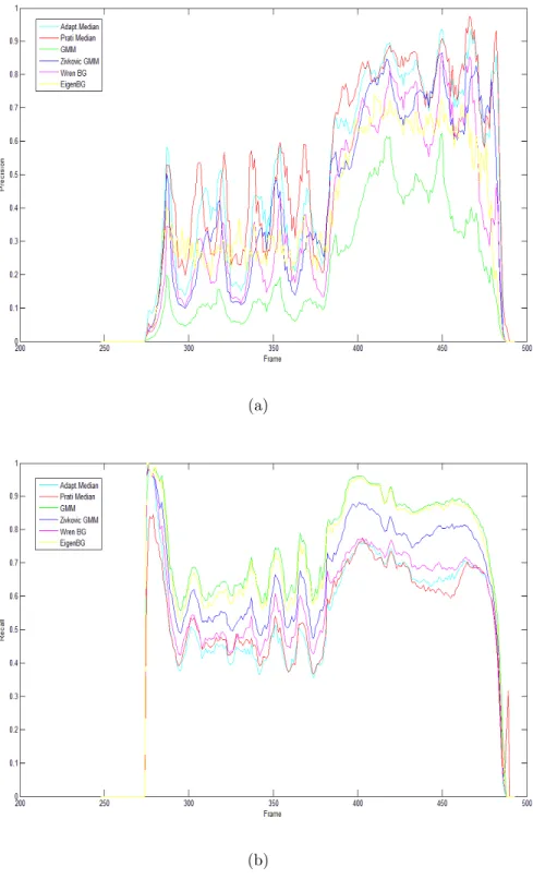
The quantitative performance of these algorithms has been evaluated us-ing ground truth data of [36]. The ground truth consists of each frame havus-ing its background and foreground pixels labeled. For this dataset, precision and recall values can be defined as [28]

P recision= ] of true positives detected

total ]of positives detected (12)

Recall = ] of true positives detected

total ] of true positives (13)

The precision chart in Fig 2.4(a) shows that P-Median and A-Median al-gorithms has higher true positives than others. This is especially observed in frames 325-500 where a person and a car are moving towards each other. The precision chart depicts that Median based approaches suppresses more pix-els which belongs to foreground while Gaussian Mixture based background subtraction algorithms accept them as foreground. This is especially unde-sired in object detection applications because noisy small misdetections can be favored over losing pixels from foreground objects, which would cause incomplete object representations.

(27)

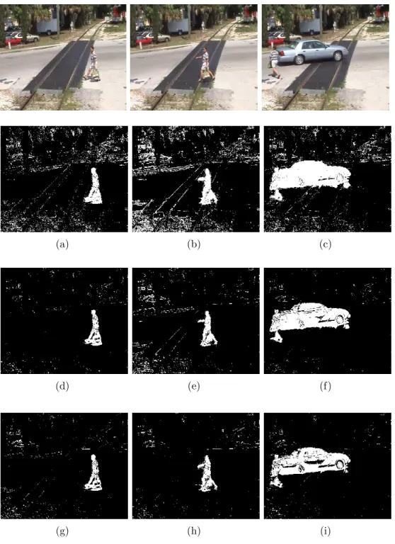
(a) (b) (c)

(d) (e) (f)

(g) (h) (i)

Figure 2.2: Rows correspond to original image and results of Adaptive Me-dian, Prati Median and EigenBackground algorithms on car scene.

(28)

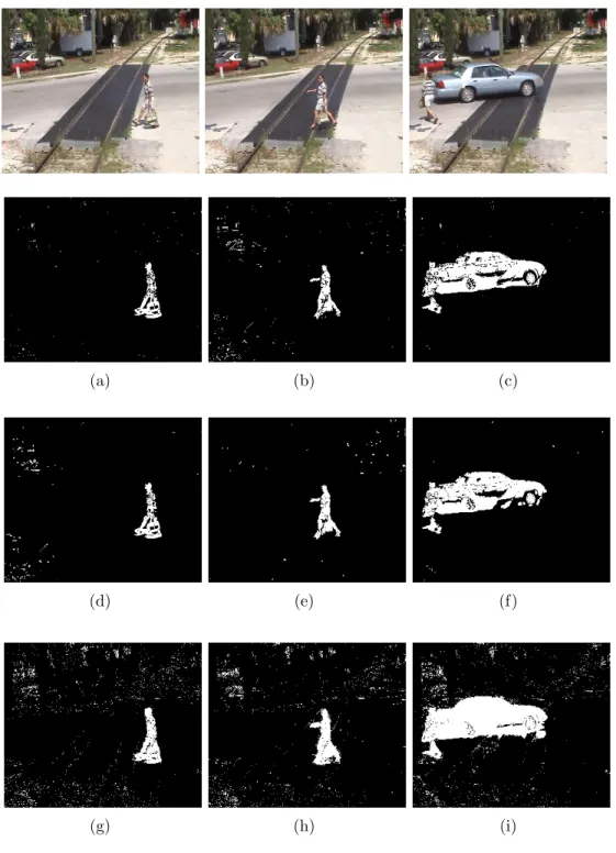
(a) (b) (c)

(d) (e) (f)

(g) (h) (i)

Figure 2.3: Rows correspond to original image Grimson GMM, Zivkovic GMM and Wren GMM algorithms respectively on car scene.

(29)

(a)

(b)

(30)

The recall values of GMM, Z-GMM and EigenBackgrounds algorithms are noticeably higher than others as shown in Figure 2.4(b). When both pre-cision and recall values are taken into account, one can comment that GMM based background subtraction algorithms found more foreground pixels than it should, containing more noise than Median based approaches. Median ap-proaches give more reliable foreground information in the data by sacrificing some low reliable foreground pixels to the background. Eigenbackgrounds algorithm shows good overall accuracy. Nevertheless the weakness of Eigen-backgrounds algorithm is that generation of a mean image for background model is computationally expensive especially for high resolution images. Nevertheless, GMM based approaches create background model in no time with K-Means parameter updates.

Conclusion of the comparative results is that Z-GMM performs superior results than all other algorithms in varying real-time conditions. However, while it performs very robust subtraction results on static scenes as shown in Figure 2.5, it can not cope with dynamic scenes effectively due to small jitters due to camera motion. The core assumption of GMM based model namely the value of each pixel is independent of its neighbours is violated in some scenarios. This encourages that either a motion stabilization algorithm needs to be utilized before running GMM algorithm or a model which takes neighboring pixel dependencies into account must be considered. The next section describes a method for obtaining background subtraction algorithm for dynamic scenes having significant camera jitter while preserving real time performance.

(31)

(a) (b) (c)

Figure 2.5: Result of GMM algorithm on Camera1 sequence obtained from PETS200 database.

2.3

Detection in Dynamic Scenes

In previous section several background subtraction algorithms have been eval-uated for real world scenes. Work of [33] showed robust and middle-way performance over other methods. Nevertheless it lacks handling dynamic scenes (see Figure 2.6). For example, an aquarium having pebbles and light-ing changes can be considered as a dynamic scene where not chooslight-ing ap-propriate number of mixture model would result in false detection results. Moreover, the same algorithm assumes there is no camera jitter. In order to overcome these two issues, we approach detection problem in dynamic scenes using nonparametric background modeling. The work described here is based on the work of Sheikh [37].

(32)

Figure 2.6: Some scenes having dynamic pixels like tree leaves, flowing water and shiny aquarium pebbles.

(r, g, b, x, y). Such a joint modeling allows sharing of color profiles of neigh-bour pixels by taking account of spatial dependency. The joint feature vector is used to create a background model:

P(x|ψb) =n−1 n

X

i=1

ϕH(x−yi) (14)

where each candidatexpixel is compared to all other pixels in the background model using ϕH kernel function in order to obtain the probability of being

a member of the background model. In the next step of the algorithm, a foreground model is constructed assuming that object’s position can not have a sudden change and most of the foreground pixels will stay as foreground in the next step. The foreground model also uses same kernel function, ϕH.

(33)

P(x|ψf) = αγ+ (1−a)m−1 m

X

i=1

ϕH(x−zi) (15)

where each candidate pixel’s foreground membership probability is a mixture of a uniform γ function and a kernel density function ϕH. The uniform

function allows new pixels which had never been encountered in background model to be added to foreground model. After obtaining model membership probabilities of a candidate pixel, the probabilities are evaluated under a Parzen classifier function:

τ =−lnP(x|ψb) P(x|ψf) =−ln n −1Pn i=1ϕH(x−yi) αγ + (1−a)m−1Pm i=1ϕH(x−zi) (16)

After computing τ values of all pixels, the final step of subtraction is basic thresholding using δ function:

δ(x) =    −1 if −lnP(x|ψb) P(x|ψf) > κ 1 otherwise (17)

The thresholded binary image represents background and foreground pixels of that frame. In each frame of the algorithm, all pixels are added to the background model but only foreground labeled pixels are added to the back-ground model. Using bimodal representation for backback-ground subtraction greatly increases variance between background and foreground distributions. Selecting one threshold using one background model is harder than selecting one threshold using one background model and a foreground model.

It is obligatory to apply a post-processing operation on the image after determining foreground pixels. The reason behind this is that due to sensorial noise or sudden illuminance change the dependency between neighbourhood

(34)

pixels can be lost resulting in misclassified pixels in the model. In literature, overcoming such a noise is possible using morphological operations, filters or global optimization over whole image using Markovian modeling. In the cited work [37] authors claimed that neighbourhood pixel dependencies can be viewed as Markov Random Field obeying Ising model and the formulation of this global optimization problem can be solved using a Graph-Cut algorithm [38], by relying on the fact that graph based energy minimization yields globals minimum on applications having two states. In their approach, τ

values obtained from Parzen classifier is fed into Graph-Cut algorithm as sink and terminal values.

While that formulation achieves optimal minimum and gets rid of many noise pixels in binary images, it is known that global optimization using GraphCut formulation is far from being real time. Using an already slow nonparametric but highly efficient modeling along with Graph-Cut formu-lation strictly constrains the method to be an offline method. However, a bottleneck in object detection module severely affects real-time capabilities of surveillance systems. The variations of GraphCut formulations are run in GPUs [39] where utilizing such special hardware may not possible for all surveillance systems.

With this motivation, we propose an alternative last step for getting rid of noise in the images. The work in literature [40] proves that if the image is subject to an average random noise, a median filter can serve as a powerful alternative and give approximately same results with MRF solution. In this work, we replace the last step of the algorithm with an edge preserving weighted median filter algorithm. The filter takes input ofτ values and sorts pixels of the image. The membership of the pixel is determined using middle

(35)

value as the threshold of the weighted filter. Using such median filter removes utilization ofδ(x) function and selecting an optimalκfunction. Results show that optimization using weighted median filter gives very successful results.

2.4

Implementation Results

The background of observed scene will change in time so background and foreground models must be updated in time. In the algorithm, a memory of M frames is kept where last pb images are used for updating background

model and last pf images are used for foreground model. Because

fore-ground model changes faster compared to the backfore-ground model, pb should

be larger. Increasing pb slows the update process of background model of

which stationary objects will take more time to be added to the background model. If kernel density function’s bandwidth is enlarged, the algorithm sup-presses foreground movement to cope with dynamism. In such a scenario, some parts of the objects can be also considered as member of background model.

In order to implement kernel density function, a 5 dimensional histogram approximation has been selected. As basic filling of histograms was not suffi-cient for high accuracy, linear binning as described in [41] was utilized. In the work [28], it is indicated that 11 fps is the upper limit where our algorithm ex-ceeds 20 fps. The implementation is single threaded but convenient for multi threaded implementation due to parallel operation. Such an implementation would further boost the real-time performance of the algorithm.

In Figure 2.4, results of implemented algorithm on aquarium scene is shown. The difficulties in this environment were colorful pebbles in the ground of aquarium, reflections of mirrors, abrupt movement of fish during

(36)

the algorithm’s learning phase (the background model is contaminated with moving objects). The pebbles in the ground of aquarium is a severe prob-lem for algorithms not taking account of neighbourhood information such as GMM and Adaptive Median background subtraction. As shown in Figure 2.4b, Adaptive Median algorithm can suppress pebbles’ dynamism however cannot detect all parts of the fish. In Figure 2.4c it is shown that all parts of the fish can be detected but pebbles’ dynamism can not be suppressed. More-over, the shadows of moving objects on the ground of aquarium is another problem to handle. In our approach, all of the fish are succesfully detected and dynamism of pebbles’ are suppressed (Fig 2.4d). In Figure 2.4, the out-put of the algorithm on railroad scene, having strong camera jitter, which was used in previous section for comparing real-time background subtraction algorithms has been also shown. It is proved that such nonparametric and retime approach has noticably less false detected pixels compared to al-gorithms in Section 2.1. The output of the algorithm on PETS sequence is shown in Figure 2.4. All objects in the scene are succesfully detected.

2.5

Discussions

In this chapter several real-time background subtraction algorithms have been compared. Results showed that state of the art GMM based algorithms outperform others. Nevertheless they show great vulnerability in dynamic scenes. To overcome this limitation a nonparametric algorithm which has showed promising results on dynamic scenes has been extended to operate in retime without losing pixel classification accuracy. The developed al-gorithm will provide infrastructure for multiple object tracking alal-gorithm mentioned in the next chapter.

(37)

(a) (b)

(c) (d)

Figure 2.7: a) An image from aquarium dataset b) Adaptive-Median based background subtraction result c) GMM based background subtraction result d) Proposed background subtraction result.

(38)

(a) Image

(b) Background Subtraction

(c) 3x3 Median Filter

(d) 5x5 Median Filter

Figure 2.8: a) Two image from aquarium dataset b) Result of Background and Foreground Modeling c) 3x3 Weighted Median Filter as last step d) 5x5 Weighted Median Filter as last step

(39)

(a) Image

Figure 2.9: a) Two image from railroad dataset b) Result of Background and Foreground Modeling c) 3x3 Weighted Median Filter as last step d) 5x5 Weighted Median Filter as last step

(40)

(a) Image

Figure 2.10: a) Two image from PETS dataset b) Result of Background and Foreground Modeling c) 3x3 Weighted Median Filter as last step d) 5x5 Weighted Median Filter as last step

(41)

Chapter III

3

Real-Time Multiple Object Tracking Using

Virtual Shells

Object tracking has been a focus of research for decades due to its promising potential for real-time applications such as intelligent user interfaces, naviga-tional systems and surveillance. A successful tracking algorithm is expected to be robust against environmental changes. Main difficulties of the single object tracking problem are appearance changes, abrupt motion and object non-rigidity. One can view multiple object tracking as the problem of run-ning multiple tracker instances on each object. However such an approach is likely to fail because of not exploiting the dependence between tracker instances and object models, running each tracker independently, causing tracker to get stuck on one object and lose the others [42]. One needs a more reliable tracker which uses holistic information exploiting the tracking correlation between objects.

Main problem of the multi object tracking systems is object interactions which give rise to occlusions [43, 44]. While simple scenarios usually include interactions of two objects, real world examples may include several objects interacting with each other that give rise to complex events and cause the tracker to fail. This necessitates development of more robust, reliable and easily scalable object tracking formulations. Argyros et. al. [45] propose

(42)

online learning of color for tracking skin. Khan et. al. [46] employ particle filtering for tracking of multiple objects. Sullivan et. al. [47] exploit con-tinuity of depth and motion direction for object labeling problem. Yu and Medioni [48] propose a Markov Chain Monte Carlo formulation for multiple object tracking.

Most of the multi object tracking methods, regardless of the number of cameras installed, requires a background subtraction algorithm to detect motion, a prerequisite step for object representation. The occlusion problem is mostly handled in two different ways: merge-split approach and straight-through approach as noted in work of Gabriel et. al. [49]. In the merge-split based methods (McKenna et. al. [50] and Bremond et. al. [51] use appearance cues, Haritaoglu’s W4 system [52] uses appearance and motion cues), separate blobs are updated as long as no occlusion is detected. In the case of occlusion, a joint blob is formed and tracked until the objects are splitted. The detection of beginning and termination of occlusion requires an occlusion and split predicate. Straight-through approaches as in Khan’s method [53] and Haritaoglu’s Hydra system [54] do not handle split and merge cases separately. These approaches continue to track each individual object in the presence of occlusions using various image features. No joint blob, or hypothesis, is formed during the occlusion phase. These methods require an occlusion predicate which acts as a trigger for ongoing occlusion event.

Regardless of the approach that may be taken, a robust and reliable multi-ple object tracking framework necessitates formal definition of the interaction problem that is boosted by merge and split predicates. Motivated by these observations, we propose a novel method for solving multiple object tracking

(43)

problem under severe occlusions. First, occlusion and split predicates are im-plemented using virtual shells and blobs. Second, a split-merge level analysis is performed using an event resolution step. This step provides information about object interactions with the help of temporal consistence. Third, a straight-through approach is adopted and pixel level analysis is carried out on shells by considering updated events without forming joint objects.

Our tracking approach has three important ingredients: a virtual shell model, an event resolution analysis and a pixel membership evaluation. By a virtual shell it is meant a closed-bounded curve or surface that encloses each object and handles complex interactions between objects that may have arbi-trary shapes and motion. An event resolution analysis based on state transi-tions is performed using geometric relatransi-tionships between object shells. This resolution step provides a macro level evaluation for multi-object tracking process. Finally, a micro level analysis, namely a pixel membership evalua-tion is carried out where all interesting pixels of objects are evaluated and assigned to corresponding objects using a probabilistic approach that utilizes virtual shells and event resolutions.

3.1

Background Subtraction

In most tracking systems, background subtraction is a preprocessing step for motion detection. In the first step of our algorithm, the background subtraction technique detailed in [37] is applied to the input frame to obtain background and foreground pixels. However, we should remark that one can use any state of the art background subtraction algorithm. For more information about background subtraction techniques for tracking purposes, the reader can check surveys [25, 55].

(44)

We use the algorithm in Chapter 2 to obtain pixel labels. As described in the previous chapter, the last step of the detection algorithm is the weighted median filter. Using such a filter guarantees reconstruction of the discon-nected parts of an object. We then utilize a condiscon-nected components labeling algorithm to obtain labeled blobs in the input image. This procedure is then continued with a geometric filtering step which is obligatory to avoid false positive regions. Geometric filtering can be utilized in many different ways. One can create a filter based on angle, shape or size constraints. In a scenario where objects with arbitrary and highly complex shapes that may undergo abrupt motion, a size filter will be adequate to remove false positives of background subtraction process. These enhanced blobs are main regions to create, track and update object hypothesis. However, due to high shape variations in temporal domain, blobs themselves are insufficient for object representation. To overcome this problem, we introduce virtual shells for further processing.

3.2

Shell Model

In shell model, each object possesses a unique enclosing shell. Shells provide spatial relaxation, allow prediction of object interactions and possible merge and split events. Object interactions can be interpreted as shell interac-tions. Object merge events are described as merging of multiple shells. Shell radius defines the interaction range for an object. An object’s interaction range is highly correlated to its speed. Thus, rapid objects will have bigger shells whereas slowing down objects’ shells will shrink in time as shown in Figure 3.1. Dynamically sized shells facilitate detection of multiple object interactions.

(45)

(a) (b)

Figure 3.1: a)An objectOi with its minimum shellSband instantaneous shell

Sr is depicted. b) Shells dynamically grow and shrink with time.

3.3

Event Resolution

Object to object relationships in the scene can be in one of three possible states: INDEPENDENT, INTERACTION and JOINT as shown in Fig 3.2. Object state transitions follow a simple but crucial assumption: no two ob-jects can make transition directly from INDEPENDENT to JOINT state or vice versa. An object in JOINT state must first move to the INTERAC-TION state before becoming INDEPENDENT objects. Thus, the tracking problem can be expressed as keeping track of the states and the positions of each object.

To be more specific, let an object Oi has an event list denoted by Li,t

at time t, that keeps record of INTERACTION (Ii,j,t) and JOINT (Ji,j,t)

relationships with object Oj. An object having no relationship with other

objects has an empty listLj,t =∅. Proposed shell model provides an

infras-tructure for the determination of possible state transitions. Let Si andSj be

the shells of the objects Oi and Oj, respectively. Also letBi and Bj denote

the blobs corresponding to Oi and Oj. In what follows, we shall consider

(46)

(a) (b)

Figure 3.2: a) State transitions of object to object relations. b) State graph where thin edges represent INTERACTION and thick edges represent JOINT relationship between objects.

• Case I.

Si∩Sj =∅, Ii,j,t−1, Ji,j,t−1 ∈/Li,t−1 (1) This condition says that if object shells do not intersect and they had no INTERACTION or JOINT relationship at time t −1, then each object is INDEPENDENT of each other.

• Case II.

Si∩Sj 6=∅, Ii,j,t−1, Ji,j,t−1 ∈/Li,t−1

Li,t =Li,t−1∪ {Ii,j,t} (2)

When two object shells has a non-empty intersection and had no IN-TERACTION and JOINT relation in their list, one can conclude that this is a start of an INTERACTION event between objects Oi andOj.

(47)

Volume of the intersection set accumulates when objects move toward each other. The INTERACTION event must be added to both objects’ event list Li,t and Lj,t.

• Case III.

Bi =Bj, Si∩Sj =6 ∅, Ii,j,t−1 ∈Li,t−1

Li,t =Li,t−1\ {Ii,j,t−1} ∪ {Ji,j,t} (3)

This equation models an incoming JOINT event. If two blobs are identical (single blob), their shells are in interaction, and they were in interaction at time t−1, then they have joined into one object. While most of the time object to object relationships can be expressed with either INDEPENDENT or INTERACTION states, JOINT state pro-vides a meaningful and necessary stage when one object fully occludes another one. At the end of occlusion, an occluded object can reappear anywhere but limited to the shell of the occluder object.

• Case IV.

Bi 6=Bj, Si∩Sj 6=∅, Ji,j,t−1 ∈Li,t−1

Li,t =Li,t−1\ {Ji,j,t−1} ∪ {Ii,j,t} (4)

Two objects in JOINT state can split in time (see Fig 3.3). On split event, their shells will have a non-empty intersection set and their blobs will be spatially distinct. The event list must be updated to hold

(48)

incom-(a)

Figure 3.3: Demonstration of Case IV (green and red) and Case V (purple and orange).

ing INTERACTION event and discard previous JOINT event between objects.

• Case V.

Si∩Sj =∅, Ii,j,t−1 ∈Li,t−1

Li,t =Li,t−1\ {Ii,j,t−1} (5) Two interacting objects end their interaction which is detected by an empty intersection set between shells. In this case both objects will go to a INDEPENDENT state and isolate themselves from each other as shown in Fig 3.3. Previous interaction record must be erased from the event list.

(49)

3.4

Pixel Membership Evaluation

After performing an event resolution analysis at object level, each object’s nearby pixels in a region of interest must be evaluated for pixel membership. This region of interest is selected as object’s shell. As in Fig. 3.3, there can be both the object pixels and the interacted objects’ pixels inside the shell radius of an object. Each pixel is then evaluated for possible membership with each object Oi using the following optimization problem.

ˆ

c(px) = arg maxcP(c|px), ∀px ∈Si, c∈ N(Lj,t) (6)

where N(.) is defined as:

N(Lj,t) ={Oi} ∪ {Oj|Oj ∈Lj,t} (7)

Note that the setN for an objectOi is defined as the union of the object

and other objects Oj that are in relations with Oi. All elements of Lj,t

are checked to determine for possible ownership of the pixel px. Then the

probability term P(c|px) can be computed by utilizing Bayes theorem; i.e.

P(c|px) = P(px|c).P(c) (8)

where the likelihood term P(px|c) is calculated using the color histogram of

pixels, and the prior term P(c) is modeled as a kernel function correspond-ing to the shell Si. In a scenario where frequent occlusions take place and

objects undergo abrupt motion, the prior term provides robustness to the pixel evaluation process by imposing the constraint of spatial proximity (to the shell center) on pixels. Pixels far away from the center will have less

(50)

attraction to belong to that shell.

(a) (b) (c)

Figure 3.4: a) Aquarium image b) Background subtraction c) Output of the event resolution and pixel membership evaluation where pixels of each object are colored differently for illustration purposes

This kernel function of each object is centered at CSi, their shell center.

Intuitively this saturation introduces some constraint where an object Oj

can not enter membership voting for a pixel if the pixel is outside of its own shell, even if it is in interaction with Oi. Selection of the kernel is a

question of accuracy and computational constraints. In our implementation, Epanechnikov kernel has been selected as the kernel function. The pixels that are far away from shell center have lower probabilities to belong to that object. The event resolution and pixel membership evaluation steps are presented in pseudo code in Algorithm 1and Algorithm 2.

As an example, in Fig 3.4, we consider an occlusion scenario between two objects. Purple colored shells indicate interaction where blue color indicate JOINT event between objects. After utilizing pixel evaluation step, green colored pixels indicate pixels of the occluded object while the blue pixels belong to the occluder.

(51)

3.5

Position Update

After assigning each pixel to the corresponding object, each object’s center is updated using member pixels; i.e.

Ci,t+1 =αE[Pi] + (1−α) ˆPCi,t+1|Ci,t (9)

where Pi represents all member pixels of Oi. The updated position is a

linear combination of the current first order moment of Pi, i.e. E[Pi], and

the Kalman filter prediction, i.e. PˆCi,t+1|Ci,t. Integration of filtering into

the process helps smooth transitions of object centers in temporal domain avoiding instantaneous noisy estimations.

3.6

Experiments

We present experiments on PETS, Caviar and aquarium sequences. Our ex-perimental aquarium setup can be seen in Figure 3.5. Aquarium images have been acquired using Imaging Source DFK21BF04H Firewire CCD cameras and resized to 320x240 resolution under RGB color space. The cameras are connected to a desktop computer, which has 2 GB memory and Intel I5 pro-cessor, through a 6-Port Firewire hub. We have also developed a graphical user interface (GUI) in QT framework to compare state of the art object de-tection and tracking algorithms (see Figure 3.5(b-c)). This GUI allows user to select and run detection and tracking algorithms on arbitrary cameras. An ongoing Mean Shift tracking algorithm [11] is depicted in Figure 3.5(b). Our graphical interface provides infrastructure for testing real-time detection and tracking algorithms.

(52)

Algorithm 1 Event Resolution

1: procedure _EventResolve(K, Lk,t−1) . Updates event list of each object

2: for k = 1→K do 3: Lk,t ←Lk,t−1 4: end for 5: for i= 1→K do 6: for j =i+ 1→K −1 do 7: if checkShellJoint(Si, Sj) then

8: if queryInteraction(Li,t−1, j) then

9: AddJi,j,t to event list Lj,t

10: Remove Ii,j,t−1 fromLj,t and Lj,t

11: end if

12: else

13: if checkShellInteraction(Si, Sj) then

14: if queryJoint(Li,t−1, j) then

15: Remove Ji,j,t−1 fromLj,t and Lj,t

16: Add Ii,j,t to Lj,t and Lj,t

17: else if !queryInteraction(Li,t−1, j) then

18: Add Ii,j,t to Lj,t and Lj,t

19: end if

20: else if queryInteraction(Li,t−1, j) then

21: Remove Ii,j,t−1 fromLj,t and Lj,t

22: end if

23: end if

24: end for

25: end for

26: return LK,t .Returns event list of each object

(53)

Algorithm 2 Pixel Membership Evaluation

1: procedure ComputePixelClasses(N, M, K) . Processes NxM image, K objects

2: for x= 1→N do

3: for y= 1 →M do

4: if I(x, y) then

5: l ← findOwnerShell( I(x, y) )

6: L←0

7: for all object inN(Ll,t) do

8: θ← compute posterior using equation (8)

9: store θ into list L

10: end for 11: b ← objectIndex(max(L)) 12: add pixel I(x, y) to Pb 13: end if 14: end for 15: end for

16: return PK . P holds each object’s pixel list

17: end procedure

act as false positives to many detection algorithms based on appearance variation. They are suppressed successfully using our background subtraction step as shown in Fig. 3.4b. Moreover, fish make abrupt motion and reflection caused by mirrors of the aquarium is another difficulty challenged in this experimental setup.

In Fig.3.6 tracker’s results on a PETS video is shown. A car and a person is moving towards each other, merges and splits after their interaction ends. In our quantitive analysis, we have used the MOTA metric described in [56] for evaluation of multiple object tracking accuracy. In Fig. 3.7, quantitative results from PETS sequence are shown where three objects (shown by blue, green, red bars) reside occasionally on the scene. We defined the tracking accuracy for each object as the distance of computed object center to the ground truth object center.

(54)

(a)

(b)

(55)

(d) (e)

Figure 3.5: Our experimental setup: aquarium environment.

A fight scene from CAVIAR database is shown in Fig. 3.8. In this scenario, two people move towards each other and start fighting. During fight as in (Fig. 3.8b-e), severe occlusions are observed in close contact. One man gets down and lies on the floor while other runs away with high speed (Fig. 3.8f-h).

In Fig. 3.9, we show a tracking sequence from our experimental setup; an aquarium containing several fish. The sequence contains rapid motion and self occlusion examples. While in many scenarios split and merge events are solved with the help of linear motion assumptions, this assumption is not valid in this environment due to abrupt and rapid motion. This is observable in Fig. 3.9e-f which shows that small fish in pink bounded box performs a sudden turn. Moreover, self-occlusion and object interactions are very frequent. In Fig. 3.9a fish in blue bounded box severely self-occludes which reduces number of pixels associated with it and suffers from a noticeable shape variation. Interaction of two fish is observable in Fig. 3.9g-h. Fish in blue box appears in front and with maneuver of neighbor fish they change

(56)

(a) (b)

(c) (d)

Figure 3.6: Sequence from PETS database.

roles, it appears behind its neighbor in a very short time.

In Fig. 3.10, we show a second sequence from aquarium environment where several objects’ interactions occur. This sequence has a total of 350 frames. In this sequence we track six fish. Four of them go into an interaction eventually(Fig.3.10i-m). Note that objects’ interaction complexity is high as many shells collide with each other and pixel classification task extends to several objects. At the end of the interaction, classification succeeds and each fish’s location is preserved (Fig. 3.10n-p). This sequence shows that arbitrary

(57)

(a)

Figure 3.7: Tracking accuracy for PETS Sequence where each color represents a tracked object.

number of objects’ interaction can be coped with using this framework. Application to UAV Video Data with the help of Video Regis-tration. Our proposed tracking approach was originally designed for sta-tionary cameras. Nevertheless, with minor modifications it can also be used for moving cameras. As a moving camera observes different regions of the scene, one must first stabilize the motion. Incoming frames can be stabilized in a fast manner using mosaicing technique proposed in Chapter 4. Note that normally, small misregistrations in stabilization process would affect profile of each pixel if we had used GMM based background subtraction as GMM does not take values of neighbour pixels into account for building up intensity profiles. However, using a KDE based background subtraction approach can cope with such small misregistration errors. We showed that KDE approach can cope with camera jitters where each pixel had motion of several pixels.

Most of the color based long term tracking algorithms suffer from illumi-nation changes. In order to cope with illumiillumi-nation changes, the color model

(58)

(a) (b)

(c) (d)

(e) (f)

(59)

(a) (b)

(c) (d)

(e) (f)

(60)

(a) (b) (c) (d)

(e) (f) (g) (h)

(i) (j) (k) (l)

(m) (n) (o) (p)

(61)

of each object needs to be updated for long tracking sequences. It is more reliable to update objects’ color model when objects have an empty event list and no occlusion. In our implementation, we have adopted linear binning for histogram filling technique as mentioned in[57] to improve binning accuracy.

3.7

Discussions

We have now presented a real-time multiple object tracking algorithm. Based on virtual shell modeling, the algorithm uses event resolution analysis and pixel class evaluation to achieve robust tracking. The algorithm has been tested on some well-known databases and also on our challenging aquarium setup where multiple objects interact with each other and create very com-plicated occlusion scenarios. Algorithm is fast, repeatable and robust. The experimental results are quite promising.

(62)

Chapter IV

4

Large Scale Mosaic of UAV Image Sequence

Image mosaicing is the process of stitching many images together in order to create a larger, consistent and seamless composite image. The composite image, having a larger field of view, can provide more information than spa-tially and temporally distinct separate images. Image mosaics are frequently used in personal, medical and remote sensing applications. Using these algo-rithms, charming panoramas of natural scenes [58] and office environment can be obtained with inexpensive off-the-shelf cameras. In the context of medical imagery, mosaicing retinal images [59] and tissues [21] produced impressive results. These algorithms are also used for creating large microscopic [60] and fingerprint imagery [61]. For remote sensing purposes, maps of an environ-ment can be created using aerial [62], underwater [63] and satellite images. They are also embedded as image stabilization and video compression rou-tines [64] in video cameras and mobile platforms. First step of virtually all mosaicing method is to perform a highly accurate local alignment between image pairs. In literature, image alignment methods can be classified into two categories as dense or sparse methods. These are also known as direct and feature based approaches [65]. In direct approaches, the whole image data is used instead of sparse features. Within these approaches, transfor-mation parameters and pixel correspondences are estimated simultaneously.

(63)

These methods have higher accuracy compared to feature based techniques as all the image information is used. Moreover, they can even exploit uniform regions where no features can be detected. While bringing high accuracy, aligned images must maintain high degree of overlap and initial estimation must be in close proximity to the solution. The pioneering work in this field is done by Lucas and Kanade [66]. A nice overview on historical progress and extensions to this framework can be found in Baker’s work [67]. As exploita-tion of the whole image data provides rich informaexploita-tion, direct approaches are widely used in problems such as mosaicing, tracking and localization. In fea-ture based methods, distinctive image feafea-tures such as SIFT [23], SURF [68] or affine invariant regions [69] are extracted. After extraction and matching of features, parameter estimation is carried out with the aid of robust esti-mation techniques. Sparsity of the input data accelerates estiesti-mation process and stimulates real-time operation. However it is troublesome to find invari-ant features in uniform regions in the image and avoid ambiguities caused by repetitive patterns. These problems are studied in the work of Mikolajczyk et al. [70]. Selecting an appropriate transformation model between images is an important step in image registration. A hierarchy of transformations [71] exist under projectivity. Although it is easier to estimate simpler mo-tion models like similarity and affine, having less parameters, these models are only valid under strong camera and scene motion constraints which limit their applicability for a general stitching algorithm. Projective homography is the most general motion model for image stitching. The model is valid un-der scene planarity or rotational motion constraints [65]. For pure rotational motion, homography is a rotation matrix that has less independent param-eters than a full homograph and as a result estimation procedure becomes

(64)

more stable [72, 58]. However, this assumption is violated at airborne ap-plications where non-negligible parallax effects are present at low altitudes. Models tackling effects of parallax have been proposed [73, 74, 75]. These plane-parallax models represent the image motion as a mixture of planar and non-planar motion. Applications of plane parallax models are presented for terrain mapping [76] and object detection with UAVs [77]. Apart from the plane-parallax framework, non-negligible parallax effects on mosaic are coped with different methods such as using Graph Cut for depth optimization [78], segmentation of parallax induced regions [79] or selection of appropriate transformations which retain good occlusion handling properties [80].

If the level of deformation between images is noticeably high, a global model may be insufficient for representation of image motion. In such a scenario, a number of local motion models can be estimated [81]. This is especially the case in medical applications where local motion models [82] are popular due to deformative structure of the organs. Although local mod-els can handle high elasticity and non-rigidity in the scene, they are cum-bersome due to computational issues making them infeasible for real-time applications.

Ultimate goal of mosaicing methods is to ensure global consistency be-tween all images in the sequence. This is important as barely linking images sequentially in time domain does neglect spatial adjacencies between im-ages. This results in accumulative error propagation through motion model. Spatio-temporal property of image sequence must be fully exploited in order to minimize misregistrations and error accumulations between images while preserving global consistency. This global update step is performed almost in all mosaicing algorithms, especially methods running on large data, either

(65)

in a delayed scheme or running concurrently with a local alignment step. Several different frameworks have been proposed to create attractive mo-saics for various scenarios. The analogy of mosaicing to simultaneous local-ization and mapping problem (SLAM) has been noted by Civera et. al. [83]. Kang formulated the problem in a graph theory framework [84]. Another suggestion is to represent the problem as a reference tracking problem [85] where a reference map reinforces the alignment process in each alignment step.

Out of all mosaicing methods, we primarily focus on mosaicing airborne imagery captured from a UAV. We are interested in the problem of stitch-ing large number of images with small amount of low parallax. There have been offline nonlinear methods for achieving very high accuracy without any timing constraints [86]. The operation can also be done in real-time since frames are taken sequentially. In light of this observation, we aim to stitch large number of images in real-time regardless of the number of images. In what follows, we will review some closely related work to our method. In this Chapter, we propose a mosaicing method for creating seamless mosaics from a set of overlapping separate images acquired from an UAV. The main contribution of our work is to reach a reasonable accuracy on the mosaic without using a computationally expensive framework such as Bundle Ad-justment. This is done by exploiting spatial relations between consecutive images and detecting intersections of multiple images using the Separating Axis Theorem (SAT). Robust estimation of homographies is done by using MLESAC (Maximum Likelihood RANSAC). The mosaic can be optionally blended to remove misregistrations and photometric defects. The flowchart of our proposed mosaicing algorithm is depicted in Figure 4.1. Proposed

(66)

method is expected to run on long image sequences where using other frame-works are inconvenient due to their limited scalability. While there are many studies [87, 88] that boost estimation process with auxiliary data, we avoid such an approach and do not perform any correction with nvisual on-board sensors. This will increase usability when sensorial data is inaccurate or unavailable. Although our method is validated on a set of overlapping images (the ratio varies between %60-%90), same algorithm can be applied to a video sequence where frame to frame overlap is very high with minor additions such as keyframe generation.

4.1

Pairwise and Warped Alignment

Image mosaicing involves transforming images captured from different cam-era poses as if they are taken from a single camcam-era and registering them on a single image plane which is the reference frame. Although there is no quanti-tative evaluation in the literature on how selection of reference frame effects quality of large scale mosaics, there has been some work to select reference frame dynamically [59]. In this work