Selection of Robust and Relevant Features for 3-D Steganalysis

(1)

Steganalysis

.

White Rose Research Online URL for this paper:

http://eprints.whiterose.ac.uk/146982/

Version: Accepted Version

Article:

Li, Zhenyu and Bors, Adrian Gheorghe orcid.org/0000-0001-7838-0021 (2018) Selection of

Robust and Relevant Features for 3-D Steganalysis. IEEE Transactions on Cybernetics.

ISSN 2168-2267

https://doi.org/10.1109/TCYB.2018.2883082

[email protected] https://eprints.whiterose.ac.uk/ Reuse

Items deposited in White Rose Research Online are protected by copyright, with all rights reserved unless indicated otherwise. They may be downloaded and/or printed for private study, or other acts as permitted by national copyright laws. The publisher or other rights holders may allow further reproduction and re-use of the full text version. This is indicated by the licence information on the White Rose Research Online record for the item.

Takedown

If you consider content in White Rose Research Online to be in breach of UK law, please notify us by

(2)

Selection of Robust and Relevant Features

for 3-D Steganalysis

Zhenyu Li and Adrian G. Bors,

Senior Member, IEEE

Department of Computer Science, University of York, York YO10 5GH, UK

Email:

{

[email protected], [email protected]

}

Abstract—While 3-D steganography and digital watermarking

represent methods for embedding information into 3-D objects, 3-D steganalysis aims to find the hidden information. Previous research studies have shown that by estimating the parameters modelling the statistics of 3-D features and feeding them into a classifier we can identify whether a 3-D object carries secret information. For training the steganalyser such features are extracted from cover and stego pairs, representing the original 3-D objects and those carrying hidden information. However, in practical applications, the steganalyzer would have to distinguish stego-objects from cover-objects, which most likely have not been used during the training. This represents a significant challenge for existing steganalyzers, raising a challenge known as the Cover Source Mismatch (CSM) problem, which is due to the significant limitation of their generalization ability. This paper proposes a novel feature selection algorithm taking into account both feature robustness and relevance in order to mitigate the CSM problem in 3-D steganalysis. In the context of the proposed methodology, new shapes are generated by distorting those used in the training. Then a subset of features is selected from a larger given set, by assessing their effectiveness in separating cover-objects from stego-cover-objects among the generated sets of cover-objects. Two different measures are used for selecting the appropriate features: Pearson Correlation Coefficient (PCC) and the Mutual Information Criterion (MIC).

Index Terms – 3-D Steganalysis; Cover Source Mismatch; Feature Selection

I. INTRODUCTION

Data hiding has many applications, including intellectual protection, marketing, storing information for contextual use and so on. Data domains used for steganography or data hiding includes audio, video and images [1], [2], [3], [4]. Steganalysis aims to identify the information which was hidden into a specific media. It relies on knowledge resulting from extracting features and analysing them as well as on computational intelligence algorithms used for information forensics and security. Various approaches have been proposed for audio and image steganalysis [5], [6], [7], [8], [9]. Steganogra-phy and information hiding into 3-D graphics have known a rapid expansion during the last decade [10], [11], [12], [13], [14], and the interest in this area will grow stronger, given the development of 3-D printing and its implications for the manufacturing industry and medicine among others. For the information embedded by a generic steganographic or information hidding algorithm, the stego-objects and cover-objects are visibly indistinguishable from each other. 3-D steganalysis aims to detect the changes embedded in shapes

and graphical models and can be seen as a classification problem which aims to distinguish the stego-objects, which carry hidden information from the cover-objects, representing the original objects. However, this is a classification of very subtle changes in the 3-D shapes, which raises new challenges. Existing 3-D steganalytic algorithms extract certain features from a large number of cover-stego pairs, representing 3-D objects before and after hiding the information into their surface [15], [16], [17]. The parameters characterizing the statistics of these features are then used as inputs for a machine learning algorithm aiming to discriminate the stego-objects from cover-objects. In this study we assess the robustness of 3-D steganalyzers in the context of the Cover Source Mismatch (CSM) problem. The CSM problem is represented by the realistic scenario that the objects used for training a steganalyzer may be originated in a cover source which is different from the one used by the steganographier for hiding the information [18]. CSM in the area of image steganalysis, was addressed during the “Break Our Steganographic System” (BOSS) contest [19]. The mismatch between the training and testing sets caused many difficulties to the participants in this contest [19], [20], [21]. In general, the CSM problem in the image domain was addressed by considering the following aspects: the training sets used, the relevant feature set to be extracted from the images, and the machine learning methods used for steganalysis.

In the case of digital images, the generalization ability of the steganalyzers is tested for images characterized by various ISO noise levels and for different JPEG compression quality factors, [22], [23]. In the context of BOSS contest, Gul and Ku-rugollu [21] proposed to use the correlation between a feature and the embedding rate as the criterion of feature selection. Meanwhile, Pasquet et al [24] proposed to use the ensemble classifier enabled with a feature selection mechanism.. The feature selection relies on evaluating the importance of each feature in the learning process [25]. A feature condensing method, called Calibrated Least Squares (CLS) was proposed in [26]. A method to mitigate the CSM due to changes in the features of the cover image was described in [27]. This approach normalizes the cover features for all steganographers by subtracting the centroid of their joint distribution. Other research studies addressing the CSM problem in images aim to find a classifier that would be robust to the variations between the training and testing data. In [28] it was shown that simple classifiers, such as the Fisher Linear Discriminant (FLD) en-semble and the Online Enen-semble Average Perceptron (OEAP)

(3)

have a better performance than more complex classifiers, when faced with the CSM problem. To mitigate the mismatch due to various changes in stego features, Ker and Pevn`y [27] and Xu et al. [23], used ensembles of classifiers which would increase the weight of those steganalytic features robust to changes.

In the machine learning community, the methods of domain adaptation [29], [30], [31], [32] and transfer learning [33], [34] have been studied in the case of various data distributions, aiming to enforce the consistency of the model information at the target domain, given a source domain. This scenario is very similar to the CSM scenario in steganalysis. Pan et al [29] proposed a feature extraction method, called Transfer Component Analysis (TCA), for domain adaptation. TCA aims to minimize the Maximum Mean Discrepancy (MMD) between samples of the source and target data in a Hilbert kernel space. Longet al[34] proposed Transfer Joint Matching (TJM), which improves TCA by jointly considering both feature matching and instance re-weighting. Zhang et al [32] proposed a unified framework that reduces the shift between domains both statistically and geometrically, referred to as the Joint Geometrical and Statistical Alignment (JGSA).

In this paper we propose the Robustness and Relevance-based Feature Selection (RRFS) algorithm for addressing the CSM problem in 3-D steganalysis. By locally distorting the surfaces of objects used for training, we extend the set of shapes. A subset of features is selected from among a larger set, based on their ability to generalize, among the enlarged database of shapes, when they are used as inputs to the steganalyzer. In this study, besides using Pearson Correlation Coefficient (PCC) [35], we also propose using the Mutual Information Criterion (MIC) in order to evaluate the relevance of each feature to the class label. Moreover, we introduce a parameter ∆ in order to control the trade-off between the features’ relevance and robustness during the feature selec-tion. The proposed methodology is tested on the Princeton Mesh Segmentation project database [36] and compared to six feature selection algorithms and three domain adaptation approaches, when considering the 3-D information hiding algorithms proposed in [10], [11], [12]. 3-D steganalysis is briefly described in Section II, while the proposed method ad-dressing the CSM problem in the context of 3-D steganalysis is explained in Section III. The experimental results are provided in Section IV and the conclusions of this study are drawn in Section V.

II. 3-D STEGANALYSIS

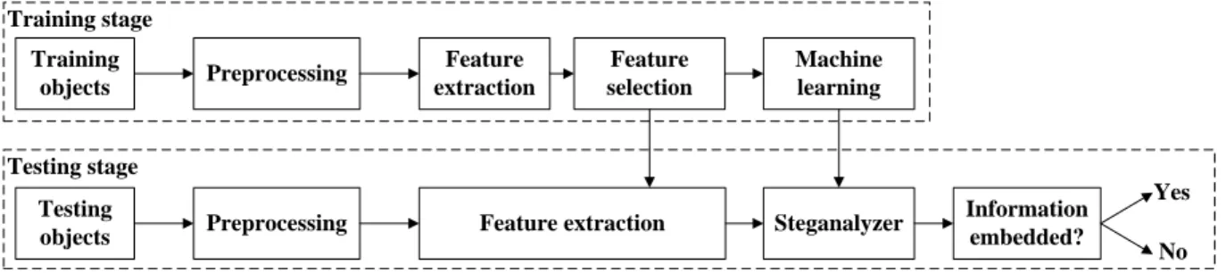
The processing stages for 3-D steganalysis are shown in the diagram from Figure 1 and they consists of the stages of training and classifying into cover-objects, representing original objects and stego-objects, representing objects where information was hidden. After a preprocessing stage, using surface smoothing and 3-D object normalization, aiming to enhance the features characteristic to the embedded informa-tion, a set of local features, characterizing the differences between 3-D shapes, are extracted from sets of 3-D objects representing both cover-objects and stego-objects. The first four statistical moments of such features are then considered as

feature vectors for training a machine learning algorithm. The 3-D steganalysis approach proposed in [15] uses the feature set YANG208, which includes the norms in the Cartesian and Laplacian coordinate system [37], the dihedral angles of the triangular surface faces and the face normals, among other features. Yang et al. [38] proposed a new steganalytic algo-rithm, specifically designed for the mean-based watermarking algorithm from [11]. Li and Bors propose the feature set LFS52 in [16], which includes the local curvature and vertex normals as steganography features, while dropping some of the other features used in [15]. Li and Bors then extended this feature set to LFS76 in [17] by adding new features such as the vertex position and the edge length in the spherical coordinate system of 3-D objects.

A very important issue, which is essential for all pattern recognition approaches, consists of the ability of the stegana-lyzer to generalize from the training set to completely different objects. The Cover Source Mismatch (CSM) problem in 3-D steganalysis addresses the robustness of steganalyzers to be trained using a set of cover and stego 3-D objects characterized by certain properties and then being able to identify the stego-objects when tested on a set of stego-objects with different surface properties. The generalization ability of exisitng steganalyzers is rather poor because the steganalytic features are sensitive to the changes of the local geometrical and topological properties of objects. So the separation boundary for the classification of cover-objects and stego-objects, calculated from a specific cover source, may not be optimal for the stego-objects origi-nating from other cover sources, resulting in a poor accuracy for the steganalyzer. In addition, we need to make it clear that the degradation of the steganalysis results under CSM is not because of the mismatch of the objects’ global shapes. The steganalytic features are designed to be sensitive to the embedding changes, which are rather small in order to be invisible, and meanwhile non-sensitive to the global shapes of the objects.

In this research study we propose a feature selection stage in order to select the robust and relevant features for training the steganalyzer in order to address the CSM problem for 3-D steganalyzers. The proposed methodology, whilst removing some of the redundant features, considers only those features that enable an appropriate generalization from the training set to the wider space of stego and cover-objects. During this stage we increase the diversity of the objects by considering local perturbations on the surface of objects. Such perturbations consists of mesh simplifications and noise additions and these would result in changes of the geometrical characteristics of the cover sources, generating objects which are quite different from the original ones when considering the local surface properties. These are then considered as cover-objects and used for hiding information through steganography resulting in sets of stego-objects. The changes produced to the surface of objects would result in statistical changes of the features used for steganalysis in both cover and stego-objects. Then, in this research study we propose to use a robust and relevance-based feature selection algorithm in order to select the best set of features for addressing the CSM problem, whilst removing the redundant features.

(4)

Testing stage Training stage Training objects Testing objects Preprocessing Preprocessing Feature extraction Feature extraction Feature selection Steganalyzer Information embedded? Machine learning Yes No

Fig. 1. The 3-D steganalysis framework based on statistical feature set selection and machine learning classifier.

During the testing stage, after using the same preprocessing steps, the selected sets of features are extracted from the testing objects. Finally, the steganalyzer decides whether any information is embedded in the given object based on the statistics of the selected features. The Quadratic Discriminant [37] and the FLD ensemble [16] have been used as machine learning methods for discriminating the cover-objects from stego-objects.

III. ROBUSTNESS ANDRELEVANCE-BASEDFEATURE

SELECTION ALGORITHM

In the following we consider that we have a set of 3-D objectsO, used for training a steganalyzer. We consider a data hiding algorithm for embedding information into the surface of these 3-D objects, representing cover-objects, resulting in stego-objects. A set of features is then extracted from both cover and stego-objects and the parameters characterizing their statistics are then used as inputs in a machine learning classifier to distinguish between the two classes of objects. The research studies from [15], [16] and [17] have found several 3-D features as being useful for 3-D steganalysis. However, the sensitivity of these 3-D features to the variation in the shape of the objects being analyzed, varies from feature to feature. The steganalytic features that are more sensitive to the embedding changes contribute more to the performance of the steganalyzer. Nevertheless, the values of these features would have a significant variation, outstripping their characteristic estimated distributions, when diversifying the cover source shapes. This ultimately leads to the degradation of the stegan-alyzer’s performance under the CSM scenario. The solution of this dilemma in the CSM scenarios would be to find a trade-off between the features’ sensitivity to the embedding changes and their robustness to the variation of the cover source. This is the motivation of the following feature selection method addressing the CSM problem in 3-D steganalysis.

The proposed feature selection algorithm, called Robustness and Relevance-based Feature Selection (RRFS), presents a mechanism for choosing the features which will guarantee the steganalysis performance in the CSM scenarios. The key idea of the proposed algorithm is to find the features that are more robust to the variation of the cover source, while preserving a relatively high sensitivity to the embedding changes, which is evaluated by their relevance to the class label. Naturally, two criteria are considered during the selection: the relevance

of the features to the class label, and the robustness of the selected feature set to the variation of the cover source. This feature selection algorithm belongs to the category of filter methods [39], shown to be efficient when used for selecting input features in various machine learning algorithms. The filter methods are suitable to be applied in the cover source mismatch situations, because they can avoid the overfitting to the training data whilst being characterized by a better generalization during the testing stage [40].

In the proposed algorithm, the relevance of the features to the class label is estimated by using the Pearson Correlation Coefficient (PCC), calculated between the distribution of each feature and the corresponding objects’ classes:

ρ(xi, y) =

cov(xi, y) σxiσy

, (1)

where xi is the i-th feature of a given feature set, X =

{xi|i = 1,2, . . . , N}, where N is the dimensionality of the input feature, y is the class label indicating either a cover-object or a stego-cover-object, cov represents the covariance and σxi is the standard deviation of xi. The Pearson correlation

coefficient can capture the linear dependency between features and the label, with |ρ(xi, y)|= 1 indicating a high degree of linearity while ρ(xi, y) = 0indicates a scattered dependency [41]. All features are ranked according to their relevance to the class label, calculated using equation (1), in descending order as:

|ρ(xi1, y)|>|ρ(xi2, y)|> . . . >|ρ(xiN, y)|, (2)

whereI={i1, i2, ...iN} is the feature index set.

In the following we also consider the Mutual Information Criterion (MIC) as a statistical measure of the relevance between each feature and the class label. MIC is known as a statistical measure of dependency between two variables. The mutual information between the i-th feature,xi, and the class label, y, is given by:

M I(xi;y) = X xi,y p(xi, y)log p(xi, y) p(xi)p(y) , (3) wherep(xi, y)is the joint probability distribution function of xi andy, andp(xi)andp(y)are the marginal probability dis-tribution functions of xi andy, respectively. Compared to the correlation coefficient, the mutual information is considered to be better in measuring the non-linear dependency between

(5)

the variables [42]. MIC was used in other feature selection methods, such as [43], [44], [45], [46].

The robustness of features to the variation of the cover source is related to solving the CSM problem. Ideally, ro-bust features should model the statistical characteristics that distinguish cover-objects and stego-objects even when these are different from those used during the training. In this study we assume that the dataset used for tests is different from that used in the training, through some transformations which are controlled in the experimental setting of this study. If the features of the objects do not change much after applying various transformations to the cover-objects, they would be ex-pected to provide similar steganalysis results to those achieved for the original cover-objects and stego-objects. Such features would have a strong robustness in the context of steganalyzers. In the following we consider changes to the surface of the objects, such as by mesh simplification and by adding noise, and compare the features extracted before and after such changes. We do not consider remeshing or surface fairing, because such operations would result in excessive smoothing and the subsequent embedding modifications will be more easily detected. Then, the Pearson correlation coefficient of the feature sets extracted before and after applying the changes to the 3-D objects is calculated as:

ρ(xi, xi,j) =

cov(xi, xi,j) σxiσxi,j

, (4)

wherexi andxi,j represent thei-th feature extracted from the original set of cover-objects O, used for training the stegan-alyzer, and from the objects obtained after applying specific transformations to the same cover source, j = 1,2, . . . , M, where M represents the number of transformations applied to the original set of cover-objects O. This formula indicates how well correlated are the initial 3-D features with those that are extracted after certain transformations. We normalize

|ρ(xi, xi,j)| to the interval [0,1]. The robustness is indicated by the average of the absolute values of the Pearson corre-lation coefficients, calculated for a specific feature i, for all j = 1, ..., M transformations: ri= 1 M M X j=1 |ρ(xi, xi,j)|, (5)

wherei= 1,2, . . . , N, andρ(xi, xi,j)is evaluated in (4). The Robustness and Relevance-based Feature Selection (RRFS) algorithm starts considering a preset number of N features as input. These are considered as those which have been proposed for 3-D steganalysis in previous studies [15], [16], [17]. The RRFS algorithm aims to find the most N′

relevant features which have relatively strong robustness to be used for a steganalyzer that addresses the CSM problem. N′

features are selected after multiple iterations through the given set of features, which are ranked each time according to their relevance, calculated by using either the equation (1) for PCC or (3) for MIC. During each iteration, a subset of featuresF′_,

with the highest relevance, is selected subject to the following conditions:

{F′_|_r

i > θq,#(F′)< N′} (6)

Algorithm 1: RRFS-PCC algorithm

Input:

Features extracted from the cover-objects and

stego-objects used for trainingX={xi|i= 1,2, ..., N}; Features extracted from other cover-sources, obtained by a shape generation procedure, and their corresponding stego-objectsXj ={xi,j|i= 1,2, ..., N, j = 1,2, ..., M}; Class labely;

Step size parameter ∆;

Dimensionality of the selected feature N′_.

Output: Index of the selected feature subsetF′_.

1 Compute the relevance of the features to the class label, ρ(xi, y) =

cov(xi,y)

σ_xiσy ;

2 Compute the Pearson correlation coefficient of two feature sets, ρ(xi, xi,j) =cov_σ(xi,xi,j)

xiσxi,j ;

3 Normalize |ρ(xi, xi,j)|to [0,1];

4 Compute the robustness of the features to the variation of the cover source, ri=_M1 PM_j₌₁|ρ(xi, xi,j)|;

5 Sort the features by relevance |ρ(x_i, y)|in the descending order and get the indexI={i1, i2, ...iN};

6 Initialize q←100−∆ and θq ←percentile({ri|i= 1,2, ...N}, q); 7 while #(F′)< N′ do 8 fork←i₁ toiN do 9 if (k /∈ F′)∧(rk> θq)∧(#(F′)< N′)then 10 Add k to F′; 11 end 12 q←q−∆; 13 θq =percentile({ri|i= 1,2, ...N}, q); 14 end 15 end 16 ReturnF′;

where θq represents the threshold for the correlation corre-sponding to the q-th percentile of set {ri|i = 1,2, . . . , N}, evaluating the robustness of the features, and #(·)represents the cardinality of a given set. Those features that are not robust enough are removed, and the RRFS algorithm then reiterates, considering the subset F′ _{containing the features}

that fulfil the required conditions. The trade-off between the robustness and the relevance of the features is controlled by a parameter∆. Initially,qis set as100−∆. After each iteration, if the cardinality of selected features #(F′₎ _{< N}′_{, then we}

reduce the threshold to a value corresponding to a percentile ofq−∆, and repeat the feature selection by considering a new thresholdθq−∆instead ofθq. When the parameter∆is closer to 0, the feature selection algorithm tends to select features which are more robust. If ∆ increases, then it will be more likely for the features with higher relevance to be selected by the RRFS algorithm. In this way, with each iteration we add additional features to the selected set of features such that whilst increasing the feature set we preserve the generalization capability of the steganalyzer. Since the features are ranked according to their relevance in descending order, the features

(6)

with higher relevance are first selected if their robustness is above the threshold θq. After each iteration, the threshold θq is gradually reduced, considering lower percentiles of q−∆ instead of q, until the dimensionality of the selected features becomes equal to N′_{. These} _N′ _{selected features are robust}

enough to the variation of the cover source whilst having a relatively high relevance to the class label at the same time. The setting of the parameter ∆ is investigated in Section IV B. The RRFS algorithm that uses PCC as the measure of the features’ relevance to the class label is named RRFS-PCC and its pseudocode is provided in Algorithm 1. Instead of using PCC, the RRFS-MIC algorithm uses MIC to calculate the features’ relevance, as defined in equation (3). The description of RRFS-MIC is similar to that of Algorithm 1.

IV. EXPERIMENTALRESULTS

In the following we provide the assessment of the proposed methodology for addressing the cover source mismatch in 3-D steganalysis. We consider 354 3-3-D objects represented as meshes which are part of the Princeton Mesh Segmentation project [36] database, which is a combination of the databases used by the European research projects, AIM@SHAPE1_, FO-CUS K3-D2_{and the shapes from the Watertight Models Track} of the SHape REtrieval Contest 2007 [47]. This database contains a large variety of shapes, representing human bodies under various postures, statues, animals, toys, tools and so on. The stego-objects are generated by applying three infor-mation hiding algorithms: 3-D Multi-Layers Steganography (MLS) proposed in [10], the blind robust watermarking algo-rithms based on modifying the Mean of the distribution of the vertices’ Radial distance coordinates in the Spherical coordi-nate system, denoted as MRS, from [11], and the Steganalysis-Resistant Watermarking (SRW) method proposed in [12]. In the case of MLS [10], the number of embedding layers is considered as 10 and the number of intervals is chosen as 10000. The relative payload ratio of each layer is nearly 1, with three vertices used for extracting the code which are not modified at all. The payload embedded by MRS from [11] is 64 bits and the watermarking strength is 0.04. We set the parameter K = 128 in SRW [12] and the upper bound of the embedding capacity as ⌊(K−2)/2⌋. Similarly to the approach from [16] we consider FLD ensembles [48], [49] as the machine learning based steganalyzer. The parameters for the FLD ensembles, such as the number of the base learner and the subspace dimensionality, are chosen as in [49]. The classifiers’ performance is measured by the detection errors which are the sums of false negatives (missed detections) and false positives (false alarms).

The initial feature set considered is a 276-dimensional fea-ture set, called LAY276, generated by combining two feafea-ture sets used for 3-D steganalysis, LFS76 [17] and YANG208 [15], counting only once the eight features which are present in both sets. We consider the initial objects of the database as cover-objects and we obtain the stego-objects following

1_{http://cordis.europa.eu/ist/kct/aimatshape synopsis.htm}

2

http://cordis.europa.eu/fp7/ict/content-knowledge/projects-focus-k3-D en.html

watermarking. In the experiments, the feature set LAY276, is initially extracted from the cover-objects and stego-objects. Then, for testing the proposed method under the CSM scenario, we apply certain transformations, such as by adding noise or by mesh simplification, to the original objects from the database and we consider the transformed objects as cover-objects for information hiding. Feature sets are extracted from these trans-formed cover-objects and their corresponding stego-objects. We consider four levels for each transformation considered, going from superficial changes to more dramatic modifications applied to the surfaces of the objects, by either increasing the level of noise, through a parameter β, representing the weight applied to the amplitude of noise, or by changing the mesh simplification factor λ, which represents the percentage of polygonal faces preserved after mesh simplification. Thus, during the calculation of the robustness, we have a set of M = 8transformations applied to the original objects. In order to test the performance of the selected features in the context of the CSM scenario, we randomly select 260 cover-objects from the original cover source and the corresponding stego-objects for training the steganalyzer. The steganalyzers are trained over the feature subsets selected by the RRFS algorithm. Then we test the steganalyzer on the other 94 pairs of cover-objects and stego-objects originated from the transformed cover sources, which have not been used during the training. The experiments are repeated 10 times with independent splits for the training and testing sets.

A. The CSM scenario

In the following, we analyze the steganalysis capability, when hiding information by means of three different infor-mation hiding algorithms. We consider both situations for a steganalyzer, when under the CSM scenario and without it. In the case when testing the steganalytic algorithm, without considering the object transformations for the CSM scenario, we utilize the whole LAY276 feature set. For diversifying the cover source space, in order to test the steganalyser under the CSM scenario, we consider two different transformations: mesh simplification and noise addition. While the first transfor-mation changes the local topology of the mesh, the latter one alters the roughness of the surface. For example these transfor-mations can simulate the distortions of the meshes caused by using different 3-D scanners when scanning the same object, because the 3-D scanners may have different accuracies and precisions, and then we may use different algorithms to create the 3-D meshes. When considering 3D printing of watermarked objects, these will also contain variations on their surface similar to those created by additive noise. When creating new shapes by considering additive noise to the mesh surface of original objects, we actually create a challenging problem for a 3-D steganalyzer, because such distortions resemble those produced to the mesh when hiding information. Thus we would actually increase the uncertainty in separating the cover-objects from stego-objects.

The mesh simplification is performed using the MATLAB function reducepatch3 which reduces the number of faces,

(7)

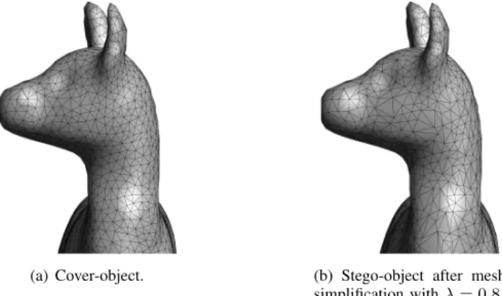
(a) Cover-object. (b) Stego-object after mesh simplification withλ= 0.8. Fig. 2. Example when using surface simplification on the cover-object to test the cover-source mismatch scenario in 3-D steganalyzers.

while aiming to preserve the overall shape of the 3-D object. The level of the simplification is controlled by the parameter λ∈ {0.98,0.95,0.9,0.8} which is interpreted as a fraction of the original number of faces. For example, if λ = 0.8, then the number of the faces is reduced to 80% of their count from the original mesh. The close-up detail of one of the original 3-D objects used in the experiments is shown in Figure 2 (a), while its corresponding stego-object obtained by using the MLS embedding algorithm after mesh simplification by a factor ofλ= 0.8, is shown in Figure 2 (b). If we would have chosen smallerλvalues, the resulting meshes would have been dramatically changed, while addressing CSM problem in 3-D steganalysis is about localized changes in the mesh surface. Be-sides, the mesh simplification algorithm used by reducepatch may produce particular artifacts, for example, it may result in the effect that the sizes of the triangles on the flat part of the simplified mesh would vary significantly. When considering uniform noise addition, its amplitude is modulated by the parameterβD, withβ∈ {1·10−5_,₂_·₁₀−5_,₃_·₁₀−5_,₅_·₁₀−5_}_,

andDis the maximum distance between the projections of any two vertices on the first principal axis, obtained by applying the Principal Component Analysis (PCA) on the original 3-D object. The application of the noise relatively to the size of the objects ensures a consistent effect for all the generated shapes, which does not depend on their initial size. With the applica-tion of various levels for the mesh simplificaapplica-tion and noise addition, we can observe the performance of the steganalytic approaches under different levels of CSM scenarios.

Figure 3 depicts the box plots for the detection errors, indi-cating their variation from the mean, for the three information hiding algorithms without CSM (Label 0) and with CSM for labels 1-8, where the diversity of objects for testing the CSM problem is produced by shape transformations through adding noise, or by mesh simplification, each by considering 4 levels of induced distortions to the original shapes. We remark that in the case without CSM (Label 0), the training set did not contain the noisy or the simplified meshes. From Figure 3 (a) it can be observed that the CSM scenario poses more challenges to steganalysis when the changes are embedded by the MLS steganographic algorithm, proposed in [10], than in

the case of the MRS [11] and SRW [12] algorithms, whose results are provided in Figures 3( b) and (c), respectively. With respect to MRS and SRW, the CSM challenge due to the diversification of shapes through mesh simplification leads to a fall in the detection of the hidden information. However, from these results, it can be observed that the CSM challenge due to the diversification of shapes through additive noise would not have much influence on the detection results. This happens because the added noise to the cover-object surface is actually smaller than the changes produced to the surface of 3-D objects by these two watermarking algorithms.

B. The analysis for selecting the parameter ∆ in the RRFS algorithm

The parameter ∆ controls the trade-off between the ro-bustness and the relevance of the features during selection, as explained in Algorithm 1 from Section III. In the follow-ing experiment, we consider the steganalysis of stego-objects carrying the information embedded by the MLS algorithm, proposed in [10], whose steganalysis results were the poorest when considering the CSM scenario in the previous section. We set ∆ ∈ {2,10,20,30,40,50}, considering the same rules as above when using RRFS-PCC algorithm for the feature selection. When∆ is small, the algorithm gives more consideration to the robustness of the features to the variation of the cover source, while when ∆ is larger it gives more consideration to the feature’s relevance to the class label. Because we consider that the robustness of the feature is very important for addressing the CSM problem, we tend to set a small value for ∆. We consider increasing the number of selected features N′ _{from 10 to 270, with steps of 10}

at each iteration. From Figure 4 we can observe that the thresholdθq decreases when increasing∆, which controls the trade-off between the robustness and relevance. A larger area under the plot of the threshold of robustness θq means more consideration is given to the features’ robustness. For example, when ∆ = 2, the selection of the features is mostly based on their robustness to the variation of the cover source.

For testing the steganalyzers, under the CSM scenario, we consider four shape alterations produced by additive noise with the amplitude given by β ∈ {1·10−5_,₃_·₁₀−5_}_, _and

by mesh simplification, considering the level of smoothing as λ ∈ {0.98,0.9}. From the plots in Figure 5 it can be observed that in the case of CSM due to noise addition, smaller values, such as ∆ ∈ {2,10,20} lead to a better performance of the steganalyzer. However, the steganalyzers with ∆ ∈ {30,40} show better generalization ability when the CSM is due to mesh simplification. Since we have to consider the CSM scenarios due to both noise addition and mesh simplifications, we set∆ = 20as a trade-off solution in the following experiments.

C. Comparison with other feature selection approaches In the following, we compare the proposed feature se-lection algorithms for steganalysis, PCC and RRFS-MIC, with filter feature selection algorithms used in pattern

(8)

Different Transformations 0 1 2 3 4 5 6 7 8 Error 0 0.1 0.2 0.3 0.4 0.5

(a) Results for MLS [10]

Different Transformations 0 1 2 3 4 5 6 7 8 Error 0 0.1 0.2 0.3 0.4 0.5 (b) Results for MRS [11] Different Transformations 0 1 2 3 4 5 6 7 8 Error 0 0.1 0.2 0.3 0.4 0.5 (c) Results for SRW [12]

Fig. 3. Box plots showing the steganalysis detection errors for the information hiding methods proposed in [10], [11], [12] when considering and without addressing the CSM challenge due to different 3-D shape modifications. Label 0 represents the results without considering the CSM challenge during the training and testing. Labels 1 to 4 indicate the results with the CSM due to additive noise at the levels ofβ∈ {1_·10−5

,2_·10−5 ,3_·10−5

,5_·10−5

}. Labels 5 to 8 indicate the results with the CSM due to mesh simplification at the level ofλ∈ {0_.98_,0_.95_,0_.9_,0_.8_}.

Dimensionality of Selected Features N'

0 20 40 60 80 100 120 140 160 180 200 220 240 260 280 Threshold of Robustness 3q 0 0.2 0.4 0.6 0.8 1 "=2 "=10 "=20 "=30 "=40 "=50

Fig. 4. Analysis of the trade-off between the relevance and robustness when selecting the features for 3-D steganalysis. The threshold of the features’ robustnessθq is varied when using the RRFS-PCC algorithm with

∆_{∈ {}2,10,20,30,40,50_} _{in order to select}N′ _{features for each split of}

the data into training and testing sets.

recognition, such as min-Redundancy and Max-Relevancy (mRMR) [46], Double Input Symmetrical Relevance (DISR) [50], Conditional Mutual Information Maximization (CMIM) [44], Infinite Feature Selection (Inf-FS) [51] and Infinite Latent Feature Selection (ILFS) [52], which have shown very good generalization ability in a wide range of applications [53]. In addition, we also compare with a simplified version of our algorithm, Relevance based Feature Selection (RFS), which selects the features with higher relevance to the class label, measured by PCC, but without considering the robustness to the variation of cover source. We repeat the steganalysis experiments, using FLD ensembles for 10 different splits of data sets and then consider the median of the resulting errors as the final test results. Figures 6, 7 and 8 show the test results when using features selected by the proposed RRFS-PCC and RRFS-MIC algorithms compared with the other six feature selection algorithms. These results are obtained

when considering the initial set of features as LAY276 for steganalysis under the CSM assumption, by considering the distortions caused by mesh simplification and uniform additive noise as in the previous section. Figure 6 shows the detection errors for the 3-D steganography MLS, proposed in [10], under the CSM scenario. As it can be observed from this figure, RRFS-PCC and RRFS-MIC algorithms achieve rather similar results, which indicates that the dependency between the 3-D features and the class label is relatively linear. Meanwhile, when compared to the other feature selection algorithms, RRFS-PCC and RRFS-MIC show better performance when the dimensionality of the selected features is within the range between 10 and 60. As the dimensionality of the selected features increases, the advantage shown by RRFS-PCC and RRFS-MIC decreases, eventually being surpassed by Inf-FS and ILFS in the CSM due to additive noise. However, Inf-FS and ILInf-FS do not provide good results in the CSM due to mesh simplification. The optimal feature dimensionality found for each CSM case, when considering a different distortion, is not always consistent with each other. Meanwhile, when considering the same type of distortion, of various intensities, for addressing the CSM problem, the resulting optimal feature dimensionalities are rather consistent with each other. For example, in the CSM due to additive noise, the minimum errors are often obtained when the dimensionality of the selected feature is between 20 and 40. Nevertheless, in the CSM due to mesh simplification, the optimal value for N′

is usually between 60 and 160. This is due to the fact that mesh simplification produces more significant shape changes than additive noise, consequently the resulting shapes requiring more features for steganalysis.

Figures 7 and 8 illustrate the steganalysis results when considering the watermarking methods, MRS and SRW, pro-posed in [11] and [12], respectively, under the CSM scenario. When considering the CSM due to additive noise, most of the feature selection algorithms show similar performance. As the dimensionality of the selected feature space increases, the detection error decreases until it eventually becomes stable. This happens because the steganalyzers are not significantly influenced by the CSM due to additive noise when identifying

(9)

Dimensionality of Selected Features N' 0 20406080 100 120 140 160 180 200 220 240 260 280 Error 0.3 0.35 0.4 0.45 0.5 "=2 "=10 "=20 "=30 "=40 "=50

(a) Noise Levelβ= 1_·10−5

Dimensionality of Selected Features N' 0 20406080 100 120 140 160 180 200 220 240 260 280 Error 0.3 0.35 0.4 0.45 0.5 "=2 "=10 "=20 "=30 "=40 "=50 (b) Noise Levelβ= 3_·10−5

Dimensionality of Selected Features N' 0 20406080 100 120 140 160 180 200 220 240 260 280 Error 0.27 0.32 0.37 0.42 0.47 "=2 "=10 "=20 "=30 "=40 "=50 (c) Simplification Levelλ= 0_.98

Dimensionality of Selected Features N' 0 204060 80 100 120 140 160 180 200 220 240 260 280 Error 0.27 0.32 0.37 0.42 0.47 "=2 "=10 "=20 "=30 "=40 "=50 (d) Simplification Levelλ= 0_.9 Fig. 5. Median values of the detection errors for MLS [10] when the steganalyzers are trained over the feature subsets selected by the RRFS-PCC with ∆∈ {2,10,20,30,40,50}in the CSM scenarios over 10 different splits of the training/testing set.

Dimensionality of Selected Features N' 0 20 40 60 80 100 120 140 160 180 200 220 240 260 280 Error 0.25 0.3 0.35 0.4 0.45 0.5 mRMR CMIM DISR Inf-FS ILFS RFS RRFS-PCC RRFS-MIC

Dimensionality of Selected Features N' 0 20 40 60 80 100 120 140 160 180 200 220 240 260 280 Error 0.25 0.3 0.35 0.4 0.45 0.5 mRMR CMIM DISR Inf-FS ILFS RFS RRFS-PCC RRFS-MIC (b) Noise Levelβ= 2_·10−5

Dimensionality of Selected Features N' 0 20 40 60 80 100 120 140 160 180 200 220 240 260 280 Error 0.25 0.3 0.35 0.4 0.45 0.5 mRMR CMIM DISR Inf-FS ILFS RFS RRFS-PCC RRFS-MIC (c) Noise Levelβ= 3_·10−5

Dimensionality of Selected Features N' 0 20 40 60 80 100 120 140 160 180 200 220 240 260 280 Error 0.25 0.3 0.35 0.4 0.45 0.5 mRMR CMIM DISR Inf-FS ILFS RFS RRFS-PCC RRFS-MIC (d) Noise Levelβ= 5_·10−5

(e) Simplification Levelλ= 0.98

Dimensionality of Selected Features N' 0 20 40 60 80 100 120 140 160 180 200 220 240 260 280 Error 0.25 0.3 0.35 0.4 0.45 0.5 mRMR CMIM DISR Inf-FS ILFS RFS RRFS-PCC RRFS-MIC (f) Simplification Levelλ= 0.95

Dimensionality of Selected Features N' 0 20 40 60 80 100 120 140 160 180 200 220 240 260 280 Error 0.25 0.3 0.35 0.4 0.45 0.5 mRMR CMIM DISR Inf-FS ILFS RFS RRFS-PCC RRFS-MIC (g) Simplification Levelλ= 0.9

Dimensionality of Selected Features N' 0 20 40 60 80 100 120 140 160 180 200 220 240 260 280 Error 0.25 0.3 0.35 0.4 0.45 0.5 mRMR CMIM DISR Inf-FS ILFS RFS RRFS-PCC RRFS-MIC (h) Simplification Levelλ= 0.8 Fig. 6. Detection errors when the information was hidden in 3-D objects by the MLS algorithm, proposed in [10], using the steganalyzers trained over the feature subsets selected by different feature selection algorithms, where the results are calculated as the median over 10 different splits of the training/testing sets.

stego-objects produced by MRS and SRW, which is validated by the results shown in Figures 3 (b) and (c). RRFS-PCC and RRFS-MIC algorithms show better performances than the other algorithms under the CSM scenario due to mesh simplification. In Figures 7 (e), (f), (g) and (h), the detec-tion errors using RRFS-PCC and RRFS-MIC are relatively constant, when the dimensionality of the feature subset N′

is in the range between 20 and 160. However, in Figures 8 (e) and (f), the detection errors when using RRFS-PCC and RRFS-MIC achieve the minimum firstly when N′ _{is around}

50. Then, the second minimum is likely to be obtained when N′_{= 130}_{. The first minimum is obtained for the most robust}

features, while the second minimum is produced because the newly added features have higher relevance than the first batch of features being considered. The fluctuation of the steganalysis error rate, whenN′ _{increases, is probably due to}

the linear dependencies and redundancy among the selected feature subsets. According to the Figures 6, 7 and 8, the

results achieved by the RRFS algorithm are better than those of the RFS indicating that the robustness of the features to the variation of cover source is essential when addressing the generalization of the steganalyzer under the CSM scenario.

In the following we provide the Receiver Operating Charac-teristic (ROC) curves for the steganalysis results in the CSM scenarios after applying the feature selection algorithms or without considering Feature Selection (FS), in Figures 9, 10 and 11. In these experiments, we identify the stego-objects produced by MLS under the CSM scenario when generating new cover-objects through additive noise with amplitude de-fined byβ∈ {1·10−5_,₃_·₁₀−5_}_{. Since the steganalysis results}

of MRS and SRW tend to be rather poor under the CSM due to mesh simplification, we consider the CSM scenarios due to mesh simplification at the levels of λ ∈ {0.98,0.9}

when detecting the stego-objects produced by MRS and SRW. When the steganalysis is carried out without feature selection, the whole feature set, LAY276, is used for training. In this

(10)

Dimensionality of Selected Features N' 0 20 40 60 80 100 120 140 160 180 200 220 240 260 280 Error 0.15 0.2 0.25 0.3 0.35 0.4 0.45 0.5 mRMR CMIM DISR Inf-FS ILFS RFS RRFS-PCC RRFS-MIC

(a) Noise Levelβ= 1·10−5

Dimensionality of Selected Features N' 0 20 40 60 80 100 120 140 160 180 200 220 240 260 280 Error 0.15 0.2 0.25 0.3 0.35 0.4 0.45 0.5 mRMR CMIM DISR Inf-FS ILFS RFS RRFS-PCC RRFS-MIC (b) Noise Levelβ= 2·10−5

Dimensionality of Selected Features N' 0 20 40 60 80 100 120 140 160 180 200 220 240 260 280 Error 0.15 0.2 0.25 0.3 0.35 0.4 0.45 0.5 mRMR CMIM DISR Inf-FS ILFS RFS RRFS-PCC RRFS-MIC (c) Noise Levelβ= 3·10−5

Dimensionality of Selected Features N' 0 20 40 60 80 100 120 140 160 180 200 220 240 260 280 Error 0.15 0.2 0.25 0.3 0.35 0.4 0.45 0.5 mRMR CMIM DISR Inf-FS ILFS RFS RRFS-PCC RRFS-MIC (d) Noise Levelβ= 5·10−5

Dimensionality of Selected Features N' 0 20 40 60 80 100 120 140 160 180 200 220 240 260 280 Error 0.15 0.2 0.25 0.3 0.35 0.4 0.45 0.5 0.55 mRMR CMIM DISR Inf-FS ILFS RFS RRFS-PCC RRFS-MIC

Dimensionality of Selected Features N' 0 20 40 60 80 100 120 140 160 180 200 220 240 260 280 Error 0.15 0.2 0.25 0.3 0.35 0.4 0.45 0.5 0.55 mRMR CMIM DISR Inf-FS ILFS RFS RRFS-PCC RRFS-MIC (f) Simplification Levelλ= 0.95

Dimensionality of Selected Features N' 0 20 40 60 80 100 120 140 160 180 200 220 240 260 280 Error 0.15 0.2 0.25 0.3 0.35 0.4 0.45 0.5 0.55 mRMR CMIM DISR Inf-FS ILFS RFS RRFS-PCC RRFS-MIC (g) Simplification Levelλ= 0.9

Dimensionality of Selected Features N' 0 20 40 60 80 100 120 140 160 180 200 220 240 260 280 Error 0.15 0.2 0.25 0.3 0.35 0.4 0.45 0.5 0.55 mRMR CMIM DISR Inf-FS ILFS RFS RRFS-PCC RRFS-MIC (h) Simplification Levelλ= 0.8 Fig. 7. Detection errors when the information was hidden in 3-D objects by the MRS algorithm, proposed in [11], using the steganalyzers trained over the feature subsets selected by different feature selection algorithms, where the results are calculated as the median over 10 different splits of the training/testing sets.

Dimensionality of Selected Features N' 0 20 40 60 80 100 120 140 160 180 200 220 240 260 280 Error 0.15 0.2 0.25 0.3 0.35 0.4 0.45 0.5 mRMR CMIM DISR Inf-FS ILFS RFS RRFS-PCC RRFS-MIC

Dimensionality of Selected Features N' 0 20 40 60 80 100 120 140 160 180 200 220 240 260 280 Error 0.15 0.2 0.25 0.3 0.35 0.4 0.45 0.5 mRMR CMIM DISR Inf-FS ILFS RFS RRFS-PCC RRFS-MIC (b) Noise Levelβ= 2_·10−5

Dimensionality of Selected Features N' 0 20 40 60 80 100 120 140 160 180 200 220 240 260 280 Error 0.15 0.2 0.25 0.3 0.35 0.4 0.45 0.5 mRMR CMIM DISR Inf-FS ILFS RFS RRFS-PCC RRFS-MIC (c) Noise Levelβ= 3_·10−5

Dimensionality of Selected Features N' 0 20 40 60 80 100 120 140 160 180 200 220 240 260 280 Error 0.15 0.2 0.25 0.3 0.35 0.4 0.45 0.5 mRMR CMIM DISR Inf-FS ILFS RFS RRFS-PCC RRFS-MIC (d) Noise Levelβ= 5_·10−5

Dimensionality of Selected Features N' 0 20 40 60 80 100 120 140 160 180 200 220 240 260 280 Error 0.25 0.3 0.35 0.4 0.45 0.5 mRMR CMIM DISR Inf-FS ILFS RFS RRFS-PCC RRFS-MIC (f) Simplification Levelλ= 0.95

Dimensionality of Selected Features N' 0 20 40 60 80 100 120 140 160 180 200 220 240 260 280 Error 0.25 0.3 0.35 0.4 0.45 0.5 mRMR CMIM DISR Inf-FS ILFS RFS RRFS-PCC RRFS-MIC (g) Simplification Levelλ= 0.9

Dimensionality of Selected Features N' 0 20 40 60 80 100 120 140 160 180 200 220 240 260 280 Error 0.25 0.3 0.35 0.4 0.45 0.5 mRMR CMIM DISR Inf-FS ILFS RFS RRFS-PCC RRFS-MIC (h) Simplification Levelλ= 0.8 Fig. 8. Detection errors when the information was hidden in 3-D objects by the SRW algorithm, proposed in [12], using the steganalyzers trained over the feature subsets selected by different feature selection algorithms, where the results are calculated as the median over 10 different splits into the training/testing sets.

(11)

False positive rate

0 0.2 0.4 0.6 0.8 1

True positive rate

0 0.2 0.4 0.6 0.8 1 Without FS DISR Inf-FS ILFS RRFS-PCC RRFS-MIC

(a) Noise Levelβ= 1·10−5

False positive rate

0 0.2 0.4 0.6 0.8 1

True positive rate

0 0.2 0.4 0.6 0.8 1 Without FS DISR Inf-FS ILFS RRFS-PCC RRFS-MIC (b) Noise Levelβ= 3·10−5

False positive rate

0 0.2 0.4 0.6 0.8 1

True positive rate

0 0.2 0.4 0.6 0.8 1 Without FS DISR Inf-FS ILFS RRFS-PCC RRFS-MIC (c) Simplification Levelλ= 0.98

False positive rate

0 0.2 0.4 0.6 0.8 1

True positive rate

0 0.2 0.4 0.6 0.8 1 Without FS DISR Inf-FS ILFS RRFS-PCC RRFS-MIC (d) Simplification Levelλ= 0.9 Fig. 9. ROC curves for the steganalysis results when the information is hidden in 3-D objects by the MLS [10] under the CSM scenario after applying the feature selection algorithms or without the Feature Selection.

False positive rate

0 0.2 0.4 0.6 0.8 1

True positive rate

(a) Simplification Levelλ= 0.98

False positive rate

0 0.2 0.4 0.6 0.8 1

True positive rate

0 0.2 0.4 0.6 0.8 1 Without FS DISR Inf-FS ILFS RRFS-PCC RRFS-MIC (b) Simplification Levelλ= 0.9 Fig. 10. ROC curves for the steganalysis results when the information is hidden in 3-D objects by the MRS [11] under the CSM scenario after applying the feature selection algorithms or without the Feature Selection.

False positive rate

0 0.2 0.4 0.6 0.8 1

True positive rate

False positive rate

0 0.2 0.4 0.6 0.8 1

True positive rate

0 0.2 0.4 0.6 0.8 1 Without FS DISR Inf-FS ILFS RRFS-PCC RRFS-MIC (b) Simplification Levelλ= 0.9 Fig. 11. ROC curves for the steganalysis results when the information is hidden in 3-D objects by the SRW [12] under the CSM scenario after applying the feature selection algorithms or without the Feature Selection.

case we consider various feature selection algorithms, such as DISR, Inf-FS and ILFS, which have shown relatively good performance on other data sets. In terms of the dimensionality of the selected feature subset, N′_{, for all the feature selection}

algorithms, we set N′ _{∈ {}₄₀_,₅₀_,₉₀_}_{, when detecting the}

stego-objects produced by MLS, MRS and SRW, respectively. The value of N′ _{is decided from the overall performance of}

the proposed feature selection algorithms in all CSM scenarios according to the results provided in Figures 6, 7 and 8. It can be observed from Figures 9, 10 and 11 that the proposed RRFS-PCC and RRFS-MIC algorithms show better performance than the other feature selection algorithms when considering the CSM scenario. Moreover, the proposed algorithms show improvement in the 3-D steganalysis results, in the context of CSM scenario, when compared to using the whole feature set. This indicates that 3-D steganalyzer’s generalization is improved when selecting a suitable feature set by the proposed RRFS-PCC and RRFS-MIC algorithms.

D. Comparison with domain adaptation approaches

In this section we compare the proposed RRFS-PCC and RRFS-MIC with several domain adaptation approaches, such as the TCA [29], TJM [34] and JGSA [32]. These domain adaptation methods have been proposed in order to address the mismatch between the training and testing data in the context of various applications, such as text classification, face recognition, object recognition, indoor WiFi localization and so on. For the proposed feature selection algorithms, we set N′ _{∈ {}₄₀_,₅₀_,₉₀_}_{, same as with the previous experiments,}

when detecting the stego-objects produced by MLS, MRS and SRW, respectively. The same values are considered for the domain adaptation methods, used for comparison. We keep the step size parameter of RRFS-PCC and RRFS-MIC, ∆ = 20, according to the conclusions of the study from Section IV.B. We consider TCA and JGSA with linear kernel, while we consider a Radial Basis Functions (RBF) kernel for TJM, and their specific parameters are chosen according to the research studies from [29], [34], [32].

We provide the Receiver Operating Characteristic (ROC) curves for the steganalysis results in the CSM scenarios after applying the proposed feature selection algorithm, domain adaptation algorithms, or without considering Feature Selec-tion, in Figures 12, 13 and 14, when considering MLS, MRS and SRW, respectively, as 3-D steganographic algorithms. It can be observed from these Figures that the proposed RRFS-PCC and RRFS-MIC algorithms provide better performance than the domain adaptation algorithms, TCA, TJM and JGSA. Moreover, the domain adaptation approaches show worse performance than the case when not using the feature selection in the CSM scenarios, as shown in Figures 13 and 14. The ineffectiveness of the typical domain adaptation approaches is due to the fact that the feature transformations applied by the domain adaptation algorithms may reduce the distances between the features from cover- and stego-objects, while they are designed to reduce the distances between the training and testing samples. In consequence, the typical domain adaptation approaches are not suitable for addressing the cover source mismatch problem in 3-D steganalysis.

(12)

0 0.2 0.4 0.6 0.8 1

False positive rate

0 0.2 0.4 0.6 0.8 1

True positive rate Without FSTCA TJM JGSA RRFS-PCC RRFS-MIC

0 0.2 0.4 0.6 0.8 1

False positive rate

0 0.2 0.4 0.6 0.8 1

True positive rate Without FSTCA TJM JGSA RRFS-PCC RRFS-MIC (b) Noise Levelβ= 3_·10−5 0 0.2 0.4 0.6 0.8 1

False positive rate

0 0.2 0.4 0.6 0.8 1

True positive rate Without FSTCA TJM JGSA RRFS-PCC RRFS-MIC (c) Simplification Levelλ= 0.98 0 0.2 0.4 0.6 0.8 1

False positive rate

0 0.2 0.4 0.6 0.8 1

(d) Simplification Levelλ= 0.9 Fig. 12. ROC curves for the steganalysis results when the information was hidden into 3-D objects by the MLS [10] under the CSM scenario after applying various domain adaptation algorithms, the proposed feature selection algorithms or without any feature selection.

0 0.2 0.4 0.6 0.8 1

False positive rate

0 0.2 0.4 0.6 0.8 1

False positive rate

0 0.2 0.4 0.6 0.8 1

True positive rate Without FS_TCA

TJM JGSA RRFS-PCC RRFS-MIC

(b) Simplification Levelλ= 0.9 Fig. 13. ROC curves for the steganalysis results when the information was hidden into 3-D objects by the MRS [11] under the CSM scenario after applying various domain adaptation algorithms, the proposed feature selection algorithms or without any feature selection.

0 0.2 0.4 0.6 0.8 1

False positive rate

0 0.2 0.4 0.6 0.8 1

False positive rate

0 0.2 0.4 0.6 0.8 1

(b) Simplification Levelλ= 0.9 Fig. 14. ROC curves for the steganalysis results when the information was hidden in 3-D objects by the SRW [12] under the CSM scenario after applying various domain adaptation algorithms, the proposed feature selection algorithms or without any feature selection.

E. Analyzing the selection of various categories of 3-D fea-tures

In the following, we analyze the contribution of various categories of features that are selected by the proposed RRFS-PCC algorithm in the CSM scenarios of 3-D steganalysis. Firstly, we categorize the steganalytic features according to their characteristics, as being either statistic or geometrical in nature. For the former category we consider grouping the features according to the statistical moments they define, as: mean, variance, skewness or kurtosis. In the latter group, we categorize the features by considering what kind of local ge-ometry characteristic they would reveal: the vertex position in the Cartesian coordinate system, the vertex norm in the Carte-sian coordinate system, the vertex position in the Laplacian coordinate system, the vertex norm in the Laplacian coordinate system, the face normal, the dihedral angle, the vertex normal, the curvature, the vertex position in the spherical coordinate system, the edge length in the spherical coordinate system. For each of these feature categories we calculate the percentage of the features being selected by the RRFS-PCC from the given pool of features when training the steganalyzers aiming to find the information hidden in 3-D objects by the algorithms, MLS [10], MRS [11], and SRW [12], under the CSM scenario where the 3-D shape domain had been extended through the additive noise and mesh simplification. The final selection ratio of every feature category is calculated as the average of 10 independent splits of the training/testing data.

Figure 15 depicts the selection ratios of all feature categories when the feature subset selected by RRFS-PCC algorithm contains a number of features which varies from 10 to 270 with a step of 10, in the context of mitigating the CSM problem. As it can be observed from Figures 15 (a), (b) and (c), when N′ _{is small, the first order moments (means) of features are}

more likely to be selected than their second order moments (variances) or than other higher order moments of the features, such as their skewness and kurtosis. It can be observed that the differences between the selection ratios of different feature categories declines as N′ _{increases. This result indicates that}

the first order moment features are the most robust and then the variance is the second most important statistical feature, when considering the context of the CSM scenario. The higher-order moments of the features considered for 3-D steganalysis are more dramatically changed than the lower-order ones under the transformations considered for testing the CSM problem.

The selection ratios of the features for the 10 geometrical categories are shown in Figures 15 (d), (e) and (f). It can be observed from Figures 15 (d), (e) and (f) that the RRFS-PCC algorithm would primarily select the curvature features (label 8) which implies that these features have the strongest robustness and relatively high relevance. This is because the curvature features model best the features of 3-D shapes within the 1-ring neighborhood of a given vertex and if one or more adjacent faces of the vertex are distorted, the other adjacent faces may average the effect and limit the influence of change on the curvature. Features originated from the vertex position (label 3) and the vertex norm (label 4) in the Laplacian coordi-nate system, as well as those originating from the vertex norm

(13)

Dimensionality of Selected Features N' 0 20 40 60 80 100 120 140 160 180 200 220 240 260 280

Accumulated Selection Ratio

0 0.5 1 1.5 2 2.5 3 3.5 4 Mean Variance Skewness Kurtosis

(a) Statistical categories of selected features in the case when the information was embedded by MLS [10].

(b) Statistical categories of selected features in the case when the information was embedded by MRS [11].

(c) Statistical categories of selected features in the case when the information was embedded by SRW [12].

0 1 2 3 4 5 6 7 8 9 10 1 2 3 4 5 6 7 8 9 10

(d) Geometrical categories of selected features when the information was embedded by MLS [10].

0 1 2 3 4 5 6 7 8 9 10 1 2 3 4 5 6 7 8 9 10

(e) Geometrical categories of selected features when the information was embedded by MRS [11]

0 1 2 3 4 5 6 7 8 9 10 1 2 3 4 5 6 7 8 9 10

(f) Geometrical categories of selected features when the information was embedded by SRW [12].

Fig. 15. The accumulated selection ratios of the features, as being discriminative between the stego-objects, created by using the embedding methods from [10], [11], [12] and their corresponding cover-objects, when using RRFS-PCC, under the specific CSM scenarios. In (a), (b) and (c), the features correspond to the first four moments of the features they characterize, such as the mean, variance, skewness, kurtosis. The meaning of the category labels in (d), (e) and (f) are: 1, vertex position in the Cartesian coordinate system; 2, vertex norm in the Cartesian coordinate system; 3, vertex position in the Laplacian coordinate system; 4, vertex norm in the Laplacian coordinate system; 5, face normal; 6, dihedral angle; 7, vertex normal; 8, curvature; 9, vertex position in the spherical coordinate system; 10, edge length in the spherical coordinate system.

(label 2) in the Cartesian coordinate system, are selected during the early stage of the feature selection, but their selection ratios remain stable for quite a while untilN′_{increases to 100, which}

indicates that the features with strong robustness are probably scattered among the various categories of geometrical features. According to Figure 15 (d), the features originated from the face normal (label 5), dihedral angle (label 6) and the vertex normal (label 7) are not selected until N′ _{reaches 60. Similar}

results are shown in Figure 15 (e). We infer that the face normals are seriously distorted by the additive noise and mesh simplification, because even when one vertex from a face is modified, the face normal would be changed as well. Since the dihedral angle and the vertex normal are calculated based on the face normal, they are unavoidably influenced by the transformations applied to extend the 3-D shape domain. It is interesting to observe that the dihedral angle features (label 6) have higher selection ratios in Figures 15 (e) and (f) than those in Figure 15 (d) during the early selection stage, when N′_{ranges from 20 to 60. This indicates that when steganalysis}

is used on the 3-D objects carrying information embedded by

various information hiding algorithms, the robustness of the features may vary significantly. With respect to the features characterizing the spherical coordinate system (labels 9 and 10), these features are also likely to be selected during the early stage of the feature selection algorithm and their selection ratios would significantly increase whenN′ _{exceeds 80.}

V. CONCLUSION

This research study proposes a solution for the cover source mismatch problem in the context of 3-D steganalysis. Ac-cording to the CSM scenario, we consider that the objects investigated during the testing stage are different from those used for training the steganalyzer. A new feature selection algorithm, called the Robustness and Relevance-based Fea-ture Selection, is proposed in this paper. Two versions of the algorithm are discussed, the first employs the Pearson Correlation Coefficient, while the second uses the Mutual Information Criterion in order to define the relevance of each feature to the class label. The robustness of the features to the variations of the cover source is evaluated by the RRFS

(14)

algorithm resulting in the selection of a feature subset which is relevant and robust to the shape variation. In order to diversify the 3-D shape variation we consider mesh simplification and additive noise for generating new cover and stego-objects when testing the steganalyzer under the CSM scenario. During the experimental analysis we consider three different information hiding methods, including a high capacity embedding method and a more recent method which embeds watermarks that cannot be detected by other steganalytic methods. The pro-posed methodology is shown to choose a better feature set than those selected by other feature selection algorithms proposed in the machine learning literature, when they are used for 3-D steganalysis in the context of CSM scenarios. Meanwhile, it also achieves better performance than several typical domain adaptation approaches when used in the CSM scenarios. A limitation of this study is that for selecting the features we consider a rather limited set of transformations when simulat-ing the CSM problem. A more general study should compare the set of cover-objects with a set of transformed objects originated from completely different cover sources than those initially used in the training stage. Moreover, it is challenging to find an optimal feature set size, which would work well for identifying stego-objects, embedded by any given information hiding algorithm, under the conditions of the CSM scenario.

REFERENCES

[1] S. Wu, J. Huang, D. Huang, and Y. Q. Shi, “Efficiently self-synchronized audio watermarking for assured audio data transmission,” IEEE Trans. on Broadcasting, vol. 51, no. 1, pp. 69–76, 2005. [2] X. Cao, L. Du, X. Wei, D. Meng, and X. Guo, “High capacity reversible

data hiding in encrypted images by patch-level sparse representation,” IEEE Trans. on Cybernetics, vol. 46, no. 5, pp. 1132–1143, 2016. [3] J. Wang, J. Ni, X. Zhang, and Y.-Q. Shi, “Rate and distortion

optimiza-tion for reversible data hiding using multiple histogram shifting,”IEEE Trans. on Cybernetics, vol. 47, no. 2, pp. 315–326, 2017.

[4] V. Sedighi, R. Cogranne, and J. Fridrich, “Content-adaptive steganogra-phy by minimizing statistical detectability,”IEEE Trans. on Information Forensics and Security, vol. 11, no. 2, pp. 221–234, 2016.

[5] Z. Li, Z. Hu, X. Luo, and B. Lu, “Embedding change rate estimation based on ensemble learning,” inProc. ACM Workshop on Information Hiding and Multimedia Security, 2013, pp. 77–84.

[6] T. D. Denemark, M. Boroumand, and J. Fridrich, “Steganalysis features for content-adaptive JPEG steganography,”IEEE Trans. on Information Forensics and Security, vol. 11, no. 8, pp. 1736–1746, 2016. [7] J. Yu, F. Li, H. Cheng, and X. Zhang, “Spatial steganalysis using

contrast of residuals,”IEEE Signal Processing Letters, vol. 23, no. 7, pp. 989–992, 2016.

[8] W. Tang, H. Li, W. Luo, and J. Huang, “Adaptive steganalysis based on embedding probabilities of pixels,” IEEE Trans. on Information Forensics and Security, vol. 11, no. 4, pp. 734–745, 2016.

[9] Y. Ren, J. Yang, J. Wang, and L. Wang, “AMR steganalysis based on second-order difference of pitch delay,” IEEE Trans. on Information Forensics and Security, vol. 12, no. 6, pp. 1345–1357, 2017. [10] M.-W. Chao, C.-H. Lin, C.-W. Yu, and T.-Y. Lee, “A high capacity 3D

steganography algorithm,”IEEE Trans. on Visualization and Computer Graphics, vol. 15, no. 2, pp. 274–284, 2009.

[11] J.-W. Cho, R. Prost, and H.-Y. Jung, “An oblivious watermarking for 3-D polygonal meshes using distribution of vertex norms,”IEEE Trans. on Signal Processing, vol. 55, no. 1, pp. 142–155, 2007.

[12] Y. Yang, R. Pintus, H. Rushmeier, and I. Ivrissimtzis, “A 3D steganalytic algorithm and steganalysis-resistant watermarking,” IEEE Trans. on Visualization and Computer Graphics, vol. 23, no. 2, pp. 1002–1013, Feb 2017.

[13] A. G. Bors and M. Luo, “Optimized 3D watermarking for minimal surface distortion,”IEEE Trans. on Image Processing, vol. 22, no. 5, pp. 1822–1835, 2013.

[14] V. Itier and W. Puech, “High capacity data hiding for 3D point clouds based on static arithmetic coding,”Multimedia Tools and Applications, vol. 76, no. 24, pp. 26 421–26 445, 2017.

[15] Y. Yang and I. Ivrissimtzis, “Mesh discriminative features for 3D steganalysis,”ACM Trans. on Multimedia Computing, Communications, and Applications, vol. 10, no. 3, pp. 27:1–27:13, 2014.

[16] Z. Li and A. G. Bors, “3D mesh steganalysis using local shape features,” inProc. IEEE Int. Conf. on Acoustics, Speech and Signal Processing (ICASSP), 2016, pp. 2144–2148.

[17] ——, “Steganalysis of 3D objects using statistics of local feature sets,” Information Sciences, vol. 415-416, pp. 85–99, 2017.

[18] A. D. Ker, P. Bas, R. B¨ohme, R. Cogranne, S. Craver, T. Filler, J. Fridrich, and T. Pevn`y, “Moving steganography and steganalysis from the laboratory into the real world,” inProc. ACM Workshop on Information Hiding and Multimedia Security, 2013, pp. 45–58. [19] P. Bas, T. Filler, and T. Pevn`y, “Break our steganographic system: The

ins and outs of orgaizing BOSS,” inProc. Int. Workshop on Information Hiding, LNCS, vol. 6958, 2011, pp. 59–70.

[20] J. Fridrich, J. Kodovsk`y, V. Holub, and M. Goljan, “Breaking HUGO– the process discovery,” inProc. Int. Workshop on Information Hiding, LNCS, vol. 6958, 2011, pp. 85–101.

[21] G. Gul and F. Kurugollu, “A new methodology in steganalysis: breaking highly undetectable steganograpy (HUGO),” inProc. Int. Workshop on Information Hiding, LNCS, vol. 6958, 2011, pp. 71–84.

[22] J. Kodovsky, V. Sedighi, and J. Fridrich, “Study of cover source mismatch in steganalysis and ways to mitigate its impact,” inProc. SPIE 9028, Media Watermarking, Security, and Forensics, 2014, p. 90280J. [23] X. Xu, J. Dong, W. Wang, and T. Tan, “Robust steganalysis based on

training set construction and ensemble classifiers weighting,” inProc. IEEE Int. Conf. on Image Processing, 2015, pp. 1498–1502. [24] J. Pasquet, S. Bringay, and M. Chaumont, “Steganalysis with

cover-source mismatch and a small learning database,” in Proc. European Signal Processing Conference, 2014, pp. 2425–2429.

[25] M. Chaumont and S. Kouider, “Steganalysis by ensemble classifiers with boosting by regression, and post-selection of features,” in Proc. IEEE Int. Conf. on Image Processing, 2012, pp. 1133–1136. [26] T. Pevn`y and A. D. Ker, “The challenges of rich features in universal

steganalysis,” inProc. SPIE 8665, Media Watermarking, Security, and Forensics, 2013, p. 86650M.

[27] A. D. Ker and T. Pevny, “A mishmash of methods for mitigating the model mismatch mess,” in Proc. SPIE 9028, Media Watermarking, Security, and Forensics, 2014, p. 90280I.

[28] I. Lubenko and A. D. Ker, “Steganalysis with mismatched covers: Do simple classifiers help?” inProc. ACM Workshop on Multimedia and Security, 2012, pp. 11–18.

[29] S. J. Pan, I. W. Tsang, J. T. Kwok, and Q. Yang, “Domain adaptation via transfer component analysis,”IEEE Trans. on Neural Networks, vol. 22, no. 2, pp. 199–210, 2011.

[30] V. M. Patel, R. Gopalan, R. Li, and R. Chellappa, “Visual domain adaptation: A survey of recent advances,” IEEE signal processing magazine, vol. 32, no. 3, pp. 53–69, 2015.

[31] M. Long, Y. Cao, J. Wang, and M. Jordan, “Learning transferable features with deep adaptation networks,” in Proc. 32nd Int. Conf. on Machine Learning (ICML), 2015, pp. 97–105.

[32] J. Zhang, W. Li, and P. Ogunbona, “Joint geometrical and statistical alignment for visual domain adaptation,” in Proceedings of the IEEE Conf. on Computer Vision and Pattern Recognition (CVPR), 2017, pp. 1859–1867.