Procedia Computer Science 91 ( 2016 ) 919 – 926
1877-0509 © 2016 Published by Elsevier B.V. This is an open access article under the CC BY-NC-ND license (http://creativecommons.org/licenses/by-nc-nd/4.0/).
Peer-review under responsibility of the Organizing Committee of ITQM 2016 doi: 10.1016/j.procs.2016.07.111
ScienceDirect
Information Technology and Quantitative Management (ITQM 2016)
A Survey on Feature Selection
Jianyu Miao
a,c, Lingfeng Niu
b,c,∗aSchool of Mathematical Sciences, University of Chinese Academy of Sciences, Beijing, 100019, China bResearch Center on Fictitious Economy&Data Science, Chinese Academy of Sciences, Beijing, 100190, China cKey Laboratory of Big Data Mining and Knowledge Management, Chinese Academy of Sciences, Beijing, 100190, China
Abstract
Feature selection, as a dimensionality reduction technique, aims to choosing a small subset of the relevant features from the original features by removing irrelevant, redundant or noisy features. Feature selection usually can lead to better learning performance, i.e., higher learning accuracy, lower computational cost, and better model interpretability. Recently, researchers from computer vision, text mining and so on have proposed a variety of feature selection algorithms and in terms of theory and experiment, show the effectiveness of their works. This paper is aimed at reviewing the state of the art on these techniques. Furthermore, a thorough experiment is conducted to check if the use of feature selection can improve the performance of learning, considering some of the approaches mentioned in the literature. The experimental results show that unsupervised feature selection algorithms benefits machine learning tasks improving the performance of clustering.
c
2016 The Authors. Published by Elsevier B.V.
Selection and/or peer-review under responsibility of ITQM2016.
Keywords: feature selection; machine learning; unsupervised; clustering 1. Introduction
Recently, available data has increased explosively in both number of samples and dimensionality in many machine learning applications such as text mining, computer vision and biomedical. In order to knowledge acquisition, it is im-portant and necessary to study how to utilize these large scale data. Our interest focus mainly on the high dimensionality of data. The huge number of high dimensional data has imposed significantly big challenge on existing machine leaning methods. Due to presence of noisy, redundant and irrelevant dimensions, they can not only make learning algorithms very slow and even degenerate the performance of learning tasks, but also can lead to difficulty on interpretability of model. Feature selection are capable of choosing a small subset of relevant features from the original ones by removing noisy, irrelevant and redundant features.
In terms of availability of label information, feature selection technique can be roughly classified into three families: supervised methods [1, 2, 3, 4], semi-supervised methods [5, 6, 7], and unsupervised methods [8, 9, 10, 11, 12]. The availability of label information allows supervised feature selection algorithms to effectively select discriminative and relevant features to distinguish samples from different classes. Some supervised methods have been proposed and studied [3, 13]. When a small portion of data is labeled, we can utilize semi-supervised feature selection which can take advantage of both labeled data and unlabeled data. Most of the existing semi-supervised feature selection algorithms [5, 14] rely on the construction of the similarity matrix and select those features that best fit the similarity matrix. Due to the absence of labels that are used for guiding the search for discriminative features, unsupervised feature selection is considered as a much harder problem [9]. In order to attain the goal of feature selection, several criteria have been proposed to evaluate feature relevance [2, 15].
Email address:[email protected] c
The Authors. Published by Elsevier B.V.
Selection and/or peer-review under responsibility of ITQM2016
∗Corresponding author. Tel.:+010-8268-0684
© 2016 Published by Elsevier B.V. This is an open access article under the CC BY-NC-ND license (http://creativecommons.org/licenses/by-nc-nd/4.0/).
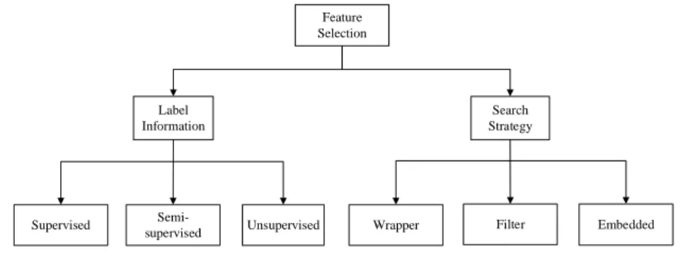
Based on the different strategies of searching, feature selection can also be classified into three methods, i.e., filter methods, wrapper methods and embedded methods. Filter methods select the most discriminative features through the character of data. Generally, filter methods perform feature selection before classification and clustering tasks and usually fall into a two-step strategy. First, all features are ranked according to certain criteria. Then, the features with the highest rankings are selected. Many filter-type methods have been used, including reliefF [16, 17],F-statistic [18], mRMR [19] and information gain [17]. Wrapper methods use the intended learning algorithm itself to evaluate the features. The work [20] utilizes Support Vector Machine methods based on Recursive Feature Elimination (RFE) to select the most relevant gene to cancers. Embedded models perform feature selection in the process of model construction. Figure 1 shows the classification of feature selection methods.
Feature Selection Label Information Search Strategy Supervised
Semi-supervised Unsupervised Wrapper Filter Embedded
Fig. 1. Feature selection category
Sparsity regularization recently is very important to make the model learned robust in machine learning and recently has been applied to feature selection. 1-SVM method [21, 22] based on1-norm regularization has been proposed to
perform feature selection. The work [23] used logistic regression with1norm regularization for feature selection. By
combining1-norm and2-norm, Hybrid Huberized SVM (HHSVM), a more structured regularization, has been proposed
in [24]. The authors in [25, 26] developed a model with2,1-norm regularization to select features shared by multi tasks.
The work [3] employed a joint2,1-norm minimization on both loss function and regularization.
The rest of paper is organized as follows. Section 2 introduces the related work. The state of the art feature selection algorithms are introduced in Section 3. In section 4, we conduct extensive experiments and report experimental results. Finally, we provide the conclusions in section 5.
2. Related work
Supervised feature selection approaches are for those data which are labeled. Traditional supervised methods such as Fisher Score [27] rank features individually according to the criterion, which can not consider the correlation among different features. Linear discriminant analysis (LDA for short) [28] was proposed to elevate features by maximizing the ratio between the class scatter and within class scatter. Unfortunately, LDA suffers from the small sample size problem because it needs to calculate the inverse matrix of within class scatter, which is singular when the number of training samples is smaller than the dimensionality of the data [29]. To avoid this problem, maximum margin criterion(MMC for short) based algorithm is proposed in [30], which uses a linear combination of traces between class scatter and within class scatter in the objective function and introduces a constraint of orthogonal weight matrix. However, all supervised methods have the common limitation of the requirement of sufficient labeled data, which is very expensive to obtain in practice. The performances of such supervised methods, however, usually drop dramatically when the labeled training data are scarce [31].
Semi-supervised feature selections, by contrast, exploit not only labeled but also unlabeled training data. As a result, semi-supervised methods are able to select features by utilizing unlabeled data when there is limited number of labeled data. Among others, graph Laplacian based semi-supervised methods assumes that most data examples lie on a low-dimensional manifold, such as semi-supervised Discriminant Analysis (SDA) [32]. In graph Laplacian based methods, graph Laplacian matrix is introduced to harness the unlabeled samples. However, they are usually less efficient on handling large-scale data because of the time-consuming computation of the graph [33]. Therefore, it is necessary and important to study unsupervised feature selection.
Due to the absence of label information that is used for guiding the search for discriminative features, unsupervised feature selection is considered as a much harder problem [9]. Many researchers have proposed some criterions to define feature relevance. One commonly used criterion is choosing those features that can best preserve the manifold structure of the original data. Another frequently used method is to seek cluster indicators through clustering algorithms and then
transform the unsupervised feature selection into a supervised framework. There are two different ways to use this method. One way is to seek cluster indicators(considered as pseudo labels) and simultaneously perform the supervised feature selection within one unified framework. The works [10] and [34] integrated nonnegative spectral cluster and structural learning into a joint framework. Another first seeks cluster indicators, then perform feature selection to remove or select certain features, and finally to repeat these two steps iteratively until certain criteria is met. The authors in [8] first use spectral analysis to obtain indicator matrix of data points, then use indicator matrix to perform feature selection like supervised one.
3. Algorithms
Before going to introduce the state of the art feature selection algorithms, we would like to give some notations to be used in our paper. We assume that we havendata pointsX= {xi}ni=1and eachxihasdfeatures{f1,f2,· · ·,fd}. And we
useXto denote as data matrix. Given a square matrixA, the trace ofAis the sum of the diagonal elements ofA. And the Frobenius norm ofA∈ m×nis given by
AF= m i=1 n j=1 A2 i j
Following the previous work [35], we give2,1norm of the matrixA∈ m×n
A2,1= m i=1 n j=1 A2 i j= m i=1 ai2
whereaiis thei-th row ofAand · 2is Euclidean norm. The affinity matrix is defined as follows
Si j= ⎧⎪⎪ ⎨ ⎪⎪⎩exp(− xi−xj2 σ2 ) xi∈ Nk(xj) orxj∈ Nk(x)i) 0 otherise
which can be used to exploit the local data structure of data points, whereNk(xj) denotes the set ofknearest neighbors of
xi. Following [36], the normalized Graph Laplacian matrix is defined asL=D−1/2(D−S)D−1/2, whereDis a diagonal
matrix, whose thei-th diagonal element is the sum of thei-th column ofS, i.e.,Dii= jSi j.
Relief [16] and its multi-class extension ReliefF [37] are supervised feature weighting algorithms of the filter model. Assuming thatpinstances are randomly sampled from data, for the case where there are two classes, the evaluation criterion of Relief is defined as S C(fi)= 1 2 p t=1 d(ft,i−fN M(xt),i)−d(ft,i−fNH(xt),i) (1)
where ft,idenotes the value of samplexton feature fi, fN M(xt),iand fNH(xt),idenote the values on thei-th feature of the
nearest points toxtwith the same and different class label, respectively.d(·) is a distance measurement. To handle
multi-class problems, the above criterion Eq.(1) can be extended to the following formulation:
S C(fi)= 1 p p t=1 ⎛ ⎜⎜⎜⎜⎜ ⎜⎜⎝− 1 mxt xj∈NH(xt) d(ft,i− fj,i)+ yyxt 1 mxt,y P(y) 1−P(yxt) xj∈N M(xt,y) d(ft,i−fj,i) ⎞ ⎟⎟⎟⎟⎟ ⎟⎟⎠ (2)
whereyxtis the class label of the instancextandP(y) is the probability of an instance being from the classy. NH(x) and
N M(x,y) denote a set of nearest points to x with the same class ofxand a different class (the classy), respectively.mxtand
mxt;yare the sizes of the setsNH(x) andN M(x,y), respectively. Usually, the size of bothNH(x) andN M(x,y),∀yyxt, is
set to a prespecified constantk. The evaluation criteria of Relief and ReliefF suggest that the two algorithms select features contributing to the separation of samples from different classes.
Laplacian Score was proposed in [15] to select features that can retain sample locality specified by an affinity matrixK. GivenK, its corresponding degree matrixDand Laplacian matrixLare obtained. Then the Laplacian Score of a feature f
is calculated in the following way:
LS= fˆ TLfˆ ˆ f Dfˆ, where ˆf = f− fTD1 1TD1 (3)
where 1 is a vector of the same size with vectorf. Since features are evaluated independently in Laplacian Score, selecting
Proposed in [2], SPEC is an extension of Laplacian Score. In SPEC, given the affinity matrixK, the degree matrix
D, and the normalized Laplacian matrixL, three evaluation criteria are proposed for weighting feature relevance in the following ways: S C1(fi)= f˜iTγ(L) ˜fi= n j=1 α2 jγ(λj) (4a) S C2(fi)= ˜ fT iγ(L) ˜fi 1−( ˜fT iξ1)2 = n j=2α2jγ(λj) n j=2α2j (4b) S C3(fi)= k j=1 (γ(2)−γ(λj))α2j (4c) where ˆfi=(D 1 2fi)· D 1
2fi)−1, (λ(j), ξ(j) is thej-th eigenvalue and the eigenvector pair ofL. αj=cosθj, whereθjis the
angle between ˆfiandξj; andγ(·) is an increasing function which is used to re-scale the eigenvalues ofLfor denoising. The
top eigenvectors ofLare the optimal soft cluster indicators of the data [36]. By comparing with these eigenvectors, SPEC selects features that assign similar values to instances that are similar according toK. In [2], it is shown that Laplacian Score is a special case of the second criterion,S C2defined in SPEC. Note that SPEC also evaluates features independently.
SPFS [38] performs feature selection by preserving sample similarity, which can handle feature redundancy. The problem can be formulated by:
min W2,1≤η n i,j=1 (xTiWWTxj−Si j)2 (5) Hereη >0 is a hyper-parameter.
MCFS [8] adopt a two-step strategy to select those features such that the multi-cluster structure of data can be best preserved. To be specific, firstly, cluster indicator can be obtained through spectral clustering(problem (6a)), then use the indicator matrix to perform feature selection(problem (6b)). Consider the two following optimization problem:
min FTF=ITr(F TLF) (6a) min wi fi−XTwi+βwi1 (6b)
wherewi1is the1norm ofwi. Since the formulation only involves a sparse eigen-problem and aL1regularized least
squares problem, problem (6) can be efficiently.
Under the assumption that the class label of input data can be predicted by a linear classifier, UDFS [10] incorporated discriminative analysis and2,1-norm minimization into a joint framework for unsupervised feature selection. Feature
selection can be performed by optimizing the following problem min
WTW=ITr(W
TXLXTW)+βW2
,1 (7)
whereβ≥0 is a regularization parameter.
NDFS [39] performs spectral clustering to learn the cluster labels of the input samples, during which the feature selection is performed simultaneously. The joint learning of the cluster labels and feature selection matrix enables NDFS to select the most discriminative features. To learn more accurate cluster labels, a nonnegative constraint is explicitly imposed to the class indicators. Its formulation is presented as follows
min
W,FTr(T
TLF)+αF−XTW2
F+βW2,1
s.t.FTF=I,F≥0 (8)
whereα≥0 andβ≥0 are balance parameters. Due to the presence of orthogonal constraint, optimization of problem (8) is difficult. NDFS use the idea of penalty function to solve the formulation.
Matrix factorization has been proven to be effective to perform feature selection. EUFS [40] embeds feature selection into a clustering algorithm via sparse learning without transformation. The problem can be formulated as
min
U,VX−UV
T2
,1+αV2,1+βTr(UTLU)
s.t.UTU=I,U≥0 (9)
whereα ≥ 0 andβ≥ 0 are balance parameters. 2,1norm is applied to cost function to reduce the effect of noise and
outliers. In order to obtain more sparse solution,2,1regularization has been used. The authors in [40] has developed a
4. Experiments
Due to the space limitation of paper, in this section, we conduct extensive experiments only for unsupervised feature selection. In our experiments, we used 12 publicly available data sets.
4.1. Datasets
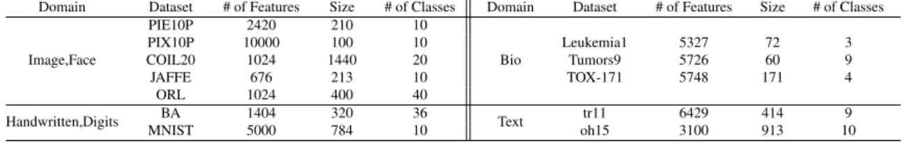
The experiments are conducted on 12 publicly available datasets, including five image datasets (PIX10P, PIE10P, COIL20, ORL and JAFFE), two handwritten digit datasets (MNISIT and BA), two text datasets (tr11 and oh15), three microarray datasets (TOX-171, Tumors9 and Leukemia1). Table 1 summarizes the statistics of these data sets.
Table 1. Datasets Description
Domain Dataset # of Features Size # of Classes Domain Dataset # of Features Size # of Classes
Image,Face PIE10P 2420 210 10 Bio PIX10P 10000 100 10 Leukemia1 5327 72 3 COIL20 1024 1440 20 Tumors9 5726 60 9 JAFFE 676 213 10 TOX-171 5748 171 4 ORL 1024 400 40 Handwritten,Digits BA 1404 320 36 Text tr11 6429 414 9 MNIST 5000 784 10 oh15 3100 913 10 4.2. Compared Algorithms
In our experiment, the state of the art unsupervised feature selection methods mentioned above have been considered. we list them as follows:
All Features: Using all features perform clustering
MaxVar: Features corresponding to the maximum variance are selected to cluster
Laplacian Score[15]: Features consistent with Gaussian Laplacian matrix are selected to best preserve the local manifold structure
SPEC[2]: Features are selected using spectral regression
SPFS-SFS[38]: The traditional forward search strategy is utilized for similarity preserving feature selection in the SPFS framework
MCFS[8]: Features are selected based on spectral analysis and sparse regression problem
UDFS[10]: Features are selected by a joint framework of discriminative analysis and2,1norm minimization
NDFS[39]: Discriminative features are selected by a joint framework of nonnegative spectral analysis and linear regres-sion with2,1norm regularization
EUFS[40]: Unsupervised feature selection which embeds feature selection into a clustering algorithm via sparse learning without transformation.
4.3. Experiment setting
Since most of feature selection algorithms selected in experiment have one or more parameters, we have to set them before conducting experiments. In order to fairly compare with each other, we choose the best result from several different parameters setting for each algorithm. In this subsection, we give parameters setting used in these algorithms. Based on [34], for Laplacian Score, SPEC, SPFS-SFS, MCFS, UDFS, NDFS and EUFS, we would like to fix the neighborhood size
Kto be 5 for all data sets. To find the best clustering results for these algorithms, a well-known technique called grid-search strategy can be used, where the parameters range from{10−8,10−6, . . . ,106,108}. In experiments, we also need to specify
the number of selected features. It is not realistic to know the optimal number of features . we empirically choose the number of selected features from{50,100,150,200,250,300}. Based on the selected features, We use K-means algorithm to cluster the data points intocgroups. Because the initial center points have great impact on performance of K-means algorithm, we conduct K-means algorithm 20 times repeatedly with random initialization. Then, we report the average results with standard deviation.
4.4. Evaluation Metrics
There are two commonly used metrics which can be used to evaluate performance of clustering. They are clustering accuracy(ACC for short) and normalized mutual information(NMI for short). Generally speaking, the larger ACC and NMI are, the better performance of clustering is. We present the concrete mathematical formulations as below.
Clustering Accuracy(Acc): Like classification accuracy, we can compare the label obtained from clustering with true label to get clustering accuracy.
Acc=
n i=1δ
(map(li),yi)
n
whereliandyiare the cluster label and true class label ofxi, respectively,nis the total number of data points,δ(x,y)
is the delta function that equals 1 ifx=yand equals 0 otherwise, and map(li) is the permutation mapping function
that maps each cluster labelrito equivalent label from data set.
Normalized Mutual Information(NMI): NMI can be used to evaluate the quality of clusters. Now given a clustering result, the NMI can be calculated with the following formulation
NMI= c i=1 c j=1 ni jlognnii jnˆj (c i=1 nilognni)( c j=1 ˆ njlognˆnj)
whereniand ˆnjdenote the number of contained in the clusterCiand class Ljfor i = 1,2. . . ,c,j = 1,2. . . ,c,
respectively, andni jis the number of data that are in the intersection between clusterCiand classLj.
4.5. Experiment Results
We give the clustering results of different methods on the 12 real life datasets in Table 2(ACC) and Table 3(NMI). The results include the average and the standard deviation of clustering accuracy and normalized mutual information, respectively. From the two tables, we can make the following several observations. First, feature selection is necessary and effective. It can not only significantly reduce the numbers of feature and make machine learning algorithms more efficient, but also can improve the performance. Secondly, in general, almost no one feature selection method can obtain the best result on all data sets.
Table 2. Clustering results of different methods on 12 data sets. The best result for each data set is highlighted in bold face.
Dataset ACC±std(%)
All Features MaxVar Laplacian Score SPFS-SFS SPEC MCFS UDFS NDFS EUFS
PIE10P 26.7±1.5 27.1±1.1 30.1±0.4 28.9±2.1 27.5±0.8 29.3±2.1 29.5±3.3 29.4±1.6 47.5±2.3 PIX10P 85.2±3.3 82.9±3.6 86.9±4.7 86.2±3.2 86.1±5.2 88.1±6.7 83.6±2.9 83.3±7.5 86.5±4.0 COIL20 62.7±3.1 61.4±1.6 62.2±1.9 64.3±2.1 65.5±3.8 65.9±2.2 65.5±2.9 63.9±2.4 66.2±2.7 ORL 49.7±3.2 50.8±1.4 49.9±2.4 50.4±1.2 51.4±2.2 57.0±3.2 53.8±3.0 57.6±1.7 50.2±2.3 JAFFE 85.3±6.1 85.5±4.2 86.2±3.7 87.1±3.3 85.9±5.1 90.7±6.1 90.5±1.4 91.0±3.4 80.1±6.2 MNIST 51.8±2.0 52.0±1.7 52.6±1.8 54.1±1.1 52.4±0.5 52.2±0.3 57.1±1.2 49.6±1.1 53.2±2.1 BA 40.9±1.6 41.7±1.3 43.3±1.9 43.9±1.4 42.7±1.1 42.9±1.8 43.8±1.6 42.9±1.8 45.6±1.4 tr11 31.8±2.2 31.4±2.4 39.5±3.2 37.6±1.2 38.0±3.1 32.1±1.8 35.5±2.1 34.6±1.4 35.5±1.9 oh15 31.6±2.7 32.2±2.1 34.7±2.4 35.2±1.9 34.2±2.0 32.5±1.3 32.6±2.4 34.5±1.7 34.2±1.9 TOX-171 42.8±2.1 42.9±1.6 43.1±1.4 44.5±0.3 40.4±0.0 42.9±1.6 45.6±1.2 46.9±1.5 42.0±1.8 Tumors9 40.8±3.7 41.2±2.6 42.3±2.6 42.9±2.7 35.8±2.4 42.4±3.6 43.3±3.5 45.6±4.6 42.2±3.9 Leukemia1 61.0±5.9 61.3±4.2 62.5±0.0 79.2±2.1 81.6±1.6 69.7±3.2 81.0±3.8 90.5±2.5 72.5±4.2
Table 3. Clustering results of different methods on 12 data sets. The best result for each data set is highlighted in bold face.
Dataset NMI±std(%)
All Features MaxVar Laplacian Score SPFS-SFS SPEC MCFS UDFS NDFS EUFS
PIE10P 25.5±3.4 28.6±2.7 30.5±2.5 30.8±0.5 25.3±1.5 31.9±3.1 49.9±2.7 30.1±3.1 49.3±1.8 PIX10P 88.0±2.1 89.1±1.6 89.8±0.7 90.0±3.2 91.0±1.9 91.7±3.1 85.6±1.9 86.8±4.5 91.5±1.3 COIL20 77.1±1.3 71.9±0.7 72.5±1.1 73.7±0.5 75.3±1.6 74.5±1.2 76.0±1.3 74.3±1.8 76.6±1.7 ORL 70.0±1.7 70.7±2.1 71.1±1.3 70.9±1.2 71.4±1.3 75.2±1.7 73.4±1.5 75.6±1.6 70.5±1.3 JAFFE 87.5±3.8 83.1±3.4 87.2±2.4 90.8±3.7 87.4±2.2 91.4±3.8 90.3±5.2 89.4±2.1 82.3±3.4 MNIST 48.9±1.0 47.6±0.4 48.1±1.0 48.9±0.4 48.3±0.4 52.0±0.2 50.0±0.9 44.8±0.5 47.5±0.7 BA 57.2±1.1 57.7±0.9 58.7±0.7 58.9±1.2 58.3±0.8 58.6±0.8 59.1±0.9 58.1±0.9 58.4±0.9 tr11 5.7±1.6 8.9±2.2 15.2±3.5 15.3±3.4 14.5±3.0 7.1±1.7 11.1±1.6 9.9±3.5 12.7±3.9 oh15 20.5±2.1 23.2±1.6 25.7±1.9 26.2±1.3 24.9±1.6 23.4±1.1 23.2±2.1 22.3±1.8 24.5±2.7 TOX-171 13.6±2.3 11.4±3.2 12.5±1.7 20.2±3.2 9.7±0.0 12.7±0.4 16.7±4.8 22.3±1.8 13.0±1.7 Tumors9 39.5±3.1 40.2±2.5 41.0±2.3 41.3±2.1 34.5±2.4 41.1±2.7 41.5±3.5 44.1±3.4 41.1±3.2 Leukemia1 37.6±10.7 36.1±5.5 36.7±0.0 49.3±2.6 58.5±1.7 53.5±1.3 59.6±4.5 66.2±7.4 61.8±0.9
5. Conclusions
This paper gives a survey on feature selection methods proposed in literature. Several state of the art feature selection methods are introduced. As we can see in our experiments, there are one or more parameters to be set. However, in practice, we do not and can not know the best parameters corresponding to the given data set. So How to select the adaptive hyper-parameters and the number of selected features are open problems and also are our future work.
Acknowledgements
The authors would like to express their sincere thanks to the associate editor and the reviewers who made great con-tributions to the improvement of this paper. This work was partially supported by National Science Foundation of Chi-na(No.71110107026, No.91546201 and No.71331005).
References
[1] L. Wolf, A. Shashua, Feature selection for unsupervised and supervised inference: The emergence of sparsity in a weight-based approach, The Journal of Machine Learning Research 6 (2005) 1855–1887.
[2] Z. Zhao, H. Liu, Spectral feature selection for supervised and unsupervised learning, in: Proceedings of the 24th international conference on Machine learning, ACM, 2007, pp. 1151–1157.
[3] F. Nie, H. Huang, X. Cai, C. H. Ding, Efficient and robust feature selection via joint ?2, 1-norms minimization, in: Advances in neural information processing systems, 2010, pp. 1813–1821.
[4] J. Li, Z. Chen, L. Wei, W. Xu, G. Kou, Feature selection via least squares support feature machine, International Journal of Information Technology & Decision Making 6 (04) (2007) 671–686.
[5] Z. Zhao, H. Liu, Semi-supervised feature selection via spectral analysis., in: SDM, SIAM, 2007, pp. 641–646.
[6] Z. Xu, I. King, M. R.-T. Lyu, R. Jin, Discriminative semi-supervised feature selection via manifold regularization, Neural Networks, IEEE Trans-actions on 21 (7) (2010) 1033–1047.
[7] P. Wang, Y. Li, B. Chen, X. Hu, J. Yan, Y. Xia, J. Yang, Proportional hybrid mechanism for population based feature selection algorithm, Interna-tional Journal of Information Technology & Decision Making (2013) 1–30.
[8] D. Cai, C. Zhang, X. He, Unsupervised feature selection for multi-cluster data, in: Proceedings of the 16th ACM SIGKDD international conference on Knowledge discovery and data mining, ACM, 2010, pp. 333–342.
[9] J. G. Dy, C. E. Brodley, Feature selection for unsupervised learning, The Journal of Machine Learning Research 5 (2004) 845–889.
[10] Y. Yang, H. T. Shen, Z. Ma, Z. Huang, X. Zhou, l2, 1-norm regularized discriminative feature selection for unsupervised learning, in: IJCAI Proceedings-International Joint Conference on Artificial Intelligence, Vol. 22, Citeseer, 2011, p. 1589.
[11] E. R. Hruschka, E. R. Hruschka Jr, T. F. Cov˜oes, N. F. Ebecken, Bayesian feature selection for clustering problems, Journal of Information & Knowledge Management 5 (04) (2006) 315–327.
[12] R. Liu, R. Rallo, Y. Cohen, Unsupervised feature selection using incremental least squares, International Journal of Information Technology & Decision Making 10 (06) (2011) 967–987.
[13] B. Krishnapuram, A. Harternink, L. Carin, M. A. Figueiredo, A bayesian approach to joint feature selection and classifier design, Pattern Analysis and Machine Intelligence, IEEE Transactions on 26 (9) (2004) 1105–1111.
[14] Q. Cheng, H. Zhou, J. Cheng, The fisher-markov selector: fast selecting maximally separable feature subset for multiclass classification with applications to high-dimensional data, Pattern Analysis and Machine Intelligence, IEEE Transactions on 33 (6) (2011) 1217–1233.
[15] X. He, D. Cai, P. Niyogi, Laplacian score for feature selection, in: Advances in neural information processing systems, 2005, pp. 507–514. [16] K. Kira, L. A. Rendell, A practical approach to feature selection, in: Proceedings of the ninth international workshop on Machine learning, 1992,
pp. 249–256.
[17] L. E. Raileanu, K. Stoffel, Theoretical comparison between the gini index and information gain criteria, Annals of Mathematics and Artificial Intelligence 41 (1) (2004) 77–93.
[18] C. Ding, H. Peng, Minimum redundancy feature selection from microarray gene expression data, Journal of bioinformatics and computational biology 3 (02) (2005) 185–205.
[19] H. Peng, F. Long, C. Ding, Feature selection based on mutual information criteria of max-dependency, max-relevance, and min-redundancy, Pattern Analysis and Machine Intelligence, IEEE Transactions on 27 (8) (2005) 1226–1238.
[20] I. Guyon, J. Weston, S. Barnhill, V. Vapnik, Gene selection for cancer classification using support vector machines, Machine learning 46 (1-3) (2002) 389–422.
[21] P. S. Bradley, O. L. Mangasarian, Feature selection via concave minimization and support vector machines., in: ICML, Vol. 98, 1998, pp. 82–90. [22] G. Fung, O. L. Mangasarian, Data selection for support vector machine classifiers, in: Proceedings of the sixth ACM SIGKDD international
conference on Knowledge discovery and data mining, ACM, 2000, pp. 64–70.
[23] A. Y. Ng, Feature selection, l 1 vs. l 2 regularization, and rotational invariance, in: Proceedings of the twenty-first international conference on Machine learning, ACM, 2004, p. 78.
[24] L. Wang, J. Zhu, H. Zou, Hybrid huberized support vector machines for microarray classification, in: Proceedings of the 24th international confer-ence on Machine learning, ACM, 2007, pp. 983–990.
[25] G. Obozinski, B. Taskar, M. Jordan, Multi-task feature selection, Statistics Department, UC Berkeley, Tech. Rep. [26] A. Evgeniou, M. Pontil, Multi-task feature learning, Advances in neural information processing systems 19 (2007) 41. [27] R. O. Duda, P. E. Hart, D. G. Stork, Pattern classification, John Wiley & Sons, 2012.
[28] R. A. Fisher, The use of multiple measurements in taxonomic problems, Annals of eugenics 7 (2) (1936) 179–188. [29] K. Fukunaga, Introduction to statistical pattern recognition, Academic press, 2013.
[30] H. Li, T. Jiang, K. Zhang, Efficient and robust feature extraction by maximum margin criterion, Neural Networks, IEEE Transactions on 17 (1) (2006) 157–165.
[31] Y. Luo, D. Tao, C. Xu, D. Li, Vector-valued multi-view semi-supervised learning for multi-label image classification, in: Proceedings of the 27th AAAI Conference on Artificial Intelligence, AAAI 2013, 2013.
[32] D. Cai, X. He, J. Han, Semi-supervised discriminant analysis, in: Computer Vision, 2007. ICCV 2007. IEEE 11th International Conference on, IEEE, 2007, pp. 1–7.
[33] X. Chang, F. Nie, Y. Yang, H. Huang, A convex formulation for semi-supervised multi-label feature selection., in: AAAI, 2014, pp. 1171–1177. [34] Z. Li, J. Liu, Y. Yang, X. Zhou, H. Lu, Clustering-guided sparse structural learning for unsupervised feature selection, Knowledge and Data
Engineering, IEEE Transactions on 26 (9) (2014) 2138–2150.
[35] C. Ding, D. Zhou, X. He, H. Zha, R 1-pca: rotational invariant l 1-norm principal component analysis for robust subspace factorization, in: Proceedings of the 23rd international conference on Machine learning, ACM, 2006, pp. 281–288.
[36] U. Von Luxburg, A tutorial on spectral clustering, Statistics and computing 17 (4) (2007) 395–416.
[37] I. Kononenko, Estimating attributes: analysis and extensions of relief, in: Machine Learning: ECML-94, Springer, 1994, pp. 171–182.
[38] Z. Zhao, L. Wang, H. Liu, J. Ye, On similarity preserving feature selection, Knowledge and Data Engineering, IEEE Transactions on 25 (3) (2013) 619–632.
[39] Z. Li, Y. Yang, J. Liu, X. Zhou, H. Lu, Unsupervised feature selection using nonnegative spectral analysis., in: AAAI, 2012.