Board of Governors of the Federal Reserve System. International Finance Discussion Papers. Number July 2010

Board of Governors of the Federal Reserve System

International Finance Discussion Papers

Number 1003

July 2010

Is There a Fiscal Free Lunch in a Liquidity Trap?

Christopher J. Erceg

and

Jesper Lindé

NOTE: International Finance Discussion Papers are preliminary materials circulated to stimulate discussion and critical comment. References in publications to International Finance Discussion Papers (other than an acknowledgment that the writer has had access to unpublished material) should be cleared with the author or authors. Recent IFDPs are available on the Web at www.federalreserve.gov/pubs/ifdp/.

Is There a Fiscal Free Lunch in a Liquidity Trap?

Federal Reserve Board

Jesper Lindé

Federal Reserve Board and CEPR First version: April 2009

This version: July 2010

Abstract

This paper uses a DSGE model to examine the e¤ects of an expansion in government spending in a liquidity trap. If the liquidity trap is very prolonged, the spending multiplier can be much larger than in normal circumstances, and the budgetary costs minimal. But given this “…scal free lunch,”it is unclear why policymakers would want to limit the size of …scal expansion. Our paper addresses this question in a model environment in which the duration of the liquidity trap is determined endogenously, and depends on the size of the …scal stimulus. We show that even if the multiplier is high for small increases in government spending, it may decrease substantially at higher spending levels; thus, it is crucial to distinguish between the marginal and average responses of output and government debt.

JEL Classi…cation: E52, E58

Keywords: Monetary Policy, Fiscal Policy, Liquidity Trap, Zero Bound Constraint, DSGE Model.

We thank Martin Bodenstein, V.V. Chari, Luca Guerrieri, and Raf Wouters for very constructive suggestions. We also thank participants at a macroeconomic modeling conference at the Bank of Italy in June 2009, at the February 2010 NBER EF&G Meeting in San Francisco, at the CEPR 18t h _{ESSIM conference in Tarragona (Spain), at the}

2010 SED Meeting in Montreal, and seminar participants at the European Central Bank, Georgetown University, University of Maryland, the Federal Reserve Banks of Cleveland and Kansas City, and the Sveriges Riksbank. Mark Clements, James Hebden, and Ray Zhong provided excellent research assistance. The views expressed in this paper are solely the responsibility of the authors and should not be interpreted as re‡ecting the views of the Board of Governors of the Federal Reserve System or of any other person associated with the Federal Reserve System. Corresponding Author: Telephone: 202-452-2575. Fax: 202-263-4850 E-mail addresses: christopher.erceg@frb.gov and jesper.l.linde@frb.gov

1. Introduction

During the past two decades, a voluminous empirical literature has attempted to gauge the e¤ects of …scal policy shocks. This literature has been instrumental in identifying the channels through which …scal policy a¤ects the economy, and, in principle, would seem a natural guidepost for policymakers seeking to assess how alternative …scal policy actions could mitigate business cycle ‡uctuations.

However, it is unclear whether estimates of the e¤ects of …scal policy from this empirical liter-ature –which focuses almost exclusively on the postwar period –should be regarded as applicable under conditions of a recession-induced liquidity trap.1 _{Keynes (1933, 1936) argued in support} of aggressive …scal expansion during the Great Depression exactly on the grounds that the …scal multiplier was likely to be much larger during a severe economic downturn than in normal times, and the burden of …nancing it correspondingly lighter.

In this paper, we use a New-Keynesian DSGE modeling framework to examine the implications of an increase in government spending for output and the government budget when monetary policy faces a liquidity trap. A key advantage of the DSGE framework is that it allows explicit consideration of how the conduct of monetary policy –and, in particular, the zero bound constraint on nominal interest rates –a¤ects the multiplier.

We begin by showing that the government spending multiplier can be ampli…ed substantially in the presence of a prolonged liquidity trap. This corroborates analysis by Eggertson (2008) and Davig and Leeper (2009), which shows that government spending can have outsized e¤ects when monetary policy allows real interest rates to fall, and recent work by Christiano, Eichenbaum and Rebelo (2009) in a model with endogenous capital accumulation.2 While our workhorse model is a variant of the Christiano, Eichenbaum and Evans (2005) and Smets-Wouters (2007) models, we show that the spending multiplier is even larger in versions that embed hand-to-mouth agents (as in 1 _{The bulk of research suggests a government spending multiplier in the range of 0.5 to slightly above unity.}

One strand of the literature – originating with Barro (1981, 1990) – has estimated the multiplier by examining the response of output to changes in military spending. This approach has typically yielded multipliers in the range of 0.5-1.0, including in recent work by Hall (2009), although Ramey (2009) estimated a somewhat higher multiplier of 1.2. As emphasized by Hall, estimates based on this approach hinge critically on the relationship between output and spending during WWII and the Korean War, and may be somewhat downward-biased due to the "command-economy” features prevalent in WWII, and because taxes were raised markedly during the Korean War. An alternative approach involves identifying the government spending multiplier using a structural VAR – as in Blanchard and Perotti (2002), and Gali, Lopez-Salido, and Valles (2007). These studies report a government spending multiplier of unity or somewhat higher (after 1-2 years), though the cross-county evidence of Perotti (2007) and Mountford and Uhlig (2008) is suggestive of a lower multiplier.

2

In contrast, Cogan et al. (2009) analyze the e¤ects of government spending shocks in the Smets-Wouters model, and conclude that the multiplier is only slightly ampli…ed under the range of liquidity trap durations that they consider, which extend between 4 and 8 quarters. Mertens and Ravn (2010) develop a stylized model which rationalizes a low and possibly negative spending multiplier in a liquidity trap in an environment with multiple equilibria driven by expectational shocks. In their model, an increase in …scal spending con…rms and reinforces the pessimistic expectations of the private sector.

Galí, López-Salido, and Vallés 2007) and …nancial frictions (as in Bernanke, Gertler, and Gilchrist 1999, and Christiano, Motto, and Rostagno 2007). Moreover, an increase in government spending against the backdrop of a deep liquidity trap puts less upward pressure on public debt than under normal circumstances, re‡ecting that the larger output response translates into much higher tax revenues.

At …rst blush, these results seem highly supportive of Keynes’argument for …scal expansion in response to a recession-induced liquidity trap –the bene…ts are extremely high, and the budgetary expense to achieve it very low. But this raises the important question of why policymakers would want to limit the magnitude of …scal expansion, and thus pass up on what appears to be a “…scal free lunch.”

Our paper addresses this question by showing that the spending multiplier in a liquidity trap decreases with the level of government spending. The novel feature of our approach is to allow the economy’s exit from a liquidity trap – and return to conventional monetary policy – to be determined endogenously, with the consequence that the multiplier depends on the size of the …scal response. Quite intuitively, a large …scal response pushes the economy out of a liquidity trap more quickly. Because the multiplier is smaller upon exiting the liquidity trap – re‡ecting that monetary policy reacts by raising real interest rates – the marginal impact of a given-sized increase in government spending on output decreases with the magnitude of the spending hike. This dependence of the government spending multiplier on the scale of …scal expansion evidently contrasts with a standard linear framework in which the multiplier is invariant to the size of the spending shock.3

The implication that the multiplier declines in the level of spending provides a potentially important rationale for limiting the size of …scal spending packages in a liquidity trap. If so, it be-comes crucial to characterize the marginal response of output and public debt to higher government spending to make informed choices about the appropriate scale of …scal intervention in a liquidity trap. A major focus of our paper consists of providing such a quantitative characterization in an array of nested DSGE models.

Section 2 analyzes the e¤ects of government spending shocks in a simple three equation New Keynesian model in which policy rates are constrained by the zero lower bound. Similar to previous research (e.g., Eggertson 2008), the liquidity trap is generated by an adverse taste shock

3

Bodenstein, Erceg, and Guerrieri (2009) show in the context of simulations of a large-scale open economy model that the contractionary e¤ect of foreign shocks on the domestic economy increases nonlinearly in the size of the shock when the domestic economy is constrained by the zero bound.

that sharply depresses the potential real interest rate. A key result of our analysis is that the government spending multiplier – measured as the contemporaneous impact on output of a very small increment in government spending –is a step function in the level of government spending. If the level of spending is su¢ ciently small, higher government spending does not a¤ect the economy’s exit date from the liquidity trap, and the multiplier is constant at a value that is higher than in a normal situation in which monetary policy would raise real interest rates. However, as spending rises to higher levels, the economy emerges from the liquidity trap more quickly, and the multiplier drops. The multiplier continues to drop discretely as government spending rises further –re‡ecting a progressive shortening of the liquidity trap –until spending is high enough to keep the economy from falling into a liquidity trap. Beyond this level of spending, the multiplier levels out at a value equal to that under normal conditions in which policy rates are unconstrained.

The simple New Keynesian model is a convenient tool for illustrating the salient role of in‡ation expectations in determining how the multiplier varies with the level of government spending. If prices are fairly responsive to marginal cost –as implied by relatively short-lived price contracts – the multiplier is extremely high for small increments to government spending, but drops quickly at higher spending levels. Thus, the large multipliers that apply to small …scal expansion should not be inferred to carry over to much larger …scal expansions, and it is particularly important to take account of the endogeneity of the multiplier under such conditions. By contrast, the multiplier function is much ‡atter if the slope of the Phillips Curve is lower, and even at low spending levels it isn’t dramatically di¤erent than in normal times.

The simple model is also convenient tool for assessing other empirically relevant factors that may a¤ect the multiplier, including implementation lags in spending. Implementation lags may dampen the multiplier signi…cantly, and even cause the multiplier to be negative if the lags are su¢ ciently long. Thus, echoing Friedman (1953), the e¢ cacy of …scal policy in macroeconomic stabilization –even in a liquidity trap –can be hampered by “long and variable lags.”

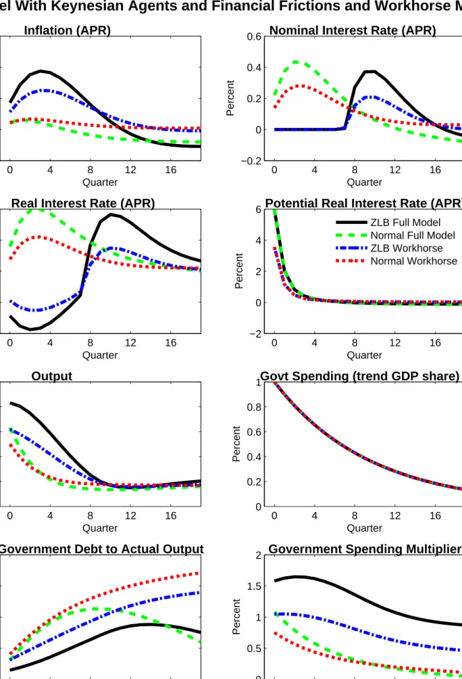
The implications of the stylized model prove useful in interpreting the behavior of the govern-ment spending multiplier in more empirically-realistic models. In Section 3, we analyze a workhorse model that is very similar to the estimated models of Christiano, Eichenbaum and Evans (2005) and Smets and Wouters (2007). Section 4 extends the workhorse model by including both “Keyne-sian”hand-to-mouth agents and …nancial frictions. These additional features boost the multiplier by amplifying the e¤ects of government spending shocks on the potential real interest rate; more-over, as argued by Galí, López-Salido, and Vallés (2007), the inclusion of Keynesian households

can help account for the positive response of private consumption to a government spending shock documented in structural VAR studies by e.g., Blanchard and Perotti (2002) and Perotti (2007).4 Given the relevance of initial conditions that determine the duration and depth of the liquidity trap for the spending multiplier, we analyze the multiplier against the backdrop of a “severe recession scenario” that attempts to capture some of the features of the U.S. experience during the recent …nancial crisis. For each model variant, such a scenario is constructed by a sequence of adverse consumption demand shocks that depress output by about 8 percent relative to steady state, and that generate a liquidity trap lasting eight quarters.

In our workhorse model, the multiplier implied by a standard-sized 1 percent of GDP increase in government spending is 1.0 in the …rst four quarters following the shock The multiplier is 1.6 in the augmented model when the share of “Keynesian”households –those that consume their entire after-tax income –equals 50 percent, which would seem at the upper end of the plausible range. Under either model variant, the multiplier is considerably larger and more persistent that under normal conditions in which monetary policy would rates interest rates immediately, and the outsized output e¤ects imply a smaller rise in government debt. Even so, the multiplier declines noticeably as the …scal spending package exceeds 2-3 percent of GDP, re‡ecting that stimulus of that magnitude is su¢ cient to reduce the duration of the liquidity trap by a couple of quarters; for example, the multiplier drops from 1.0 to 0.7 in the workhorse model. Moreover, implementation lags can markedly reduce the multiplier. Thus, against the backdrop of an eight quarter liquidity trap, there may be substantial bene…ts of increasing some forms of spending that have short implementation lags; but arguments favoring such programs based on an outsized multiplier would seem to apply only for spending packages fairly modest in scale.

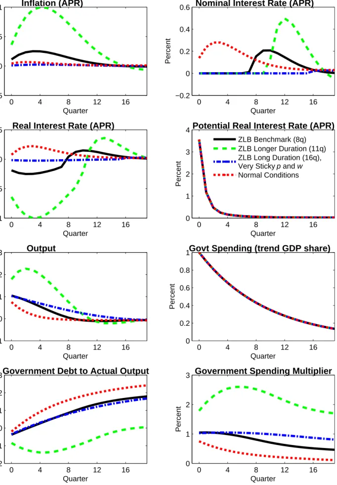
The government spending multiplier under our benchmark calibration increases markedly as the liquidity trap duration extends much beyond two years, mainly re‡ecting that expected in‡ation becomes much more responsive to shocks. With the high multiplier, government debt falls sharply, so that the …scal expansion more than pays for itself. However, while such conditions of deep recession provide a strong rationale for …scal activism, our analysis shows that the multiplier under these conditions tends to drop sharply in the level of government spending. For example, in the workhorse model with an 11 quarter liquidity trap, the multiplier is 3.3 for small increases in 4 _{As discussed in recent papers by Leeper, Walker and Yang (2009) and Ramey (2009), identi…ed VARs can}

produce misleading results if some of the …scal expansion is anticipated. Accordingly, Fisher and Peters (2009) identify government spending shocks with statistical innovations to the accumulated excess returns of large U.S. military contractors, and …nd that positive spending shocks are associated with an output multiplier above unity and increases in hours and consumption.

government spending, but declines to 1.2 as spending rises above 2 percent of GDP. Intuitively, just as small adverse shocks can exert a large contractionary impact in a long-lived liquidity trap and deep recession, small …scal expansions may be highly e¤ective in mitigating the recession; but with a shallower recession, the bene…ts of additional stimulus drop substantially.

We conduct extensive sensitivity analysis to assess how the relationship between the multiplier and level of government spending is a¤ected by the slopes of the price- and wage-setting schedules. Our benchmark calibration implies a fairly sluggish price and wage adjustment, with the slopes of the price- and wage-setting schedules at the lower end of empirical estimates: for example, price contracts have an e¤ective duration of ten quarters.5 Ifbothprices and wages were more responsive, the multiplier could be very high even for a liquidity trap lasting under two years; under such conditions, …scal policy would be a very potent tool for reversing the sizeable de‡ationary pressures that would occur in the wake of recession.6 However, the multiplier also drops abruptly with the size of the …scal stimulus, as greater stimulus shortens the duration of the liquidity trap. Thus, with four quarter price and wage contracts, the multiplier exceeds10in our workhorse model for a very small increase in spending, but drops to unity when government spending is boosted more than 1 percent of GDP. Given the resilence of short-run expected in‡ation during the past recession, we are somewhat skeptical of calibrations that imply such extreme variations in the multiplier across spending levels. But at the least, our analysis underscores that the multiplier tends to decline sharply in the level of government spending under exactly the same conditions that are favorable to a high multiplier, i.e., when expected in‡ation is highly responsive.

Taken together, our results suggest a somewhat nuanced view of the role of …scal policy in a liquidity trap. For an economy facing a deep recession that appears likely to keep monetary policy constrained by the zero bound for well over two years, there is a strong argument for increasing government spending on a temporary basis. Consistent with the views originally espoused by Keynes, this temporary boost can have much larger e¤ects than under usual conditions, and comes at a low cost to the Treasury. But as the multiplier can drop quickly with the level of …scal spending, larger spending programs may su¤er from sharply diminishing returns, and may increase government debt at the margin. Against the backdrop of a shorter-lived liquidity trap of less than two years, the multiplier is probably only slightly above unity even in the ideal situation in 5 _{We stress that the implied slope of the Phillips Curve is consistent with empirical estimates (albeit at the lower}

end). In this paper, we …nd it convenient to simply map a given slope of the Phillips curve into an e¤ective contract duration under the assumption that marginal costs are identical across …rms. However, the same slope of the Phillips curve can be consistent with a much shorter price contract duration if capital is …rm-speci…c, as shown by e.g. Galí, Gertler, and López-Salido (2001) and Altig, Christiano, Eichenbaum and Lindé (2010).

6

which …scal stimulus can be implemented immediately. Such an environment clearly presents more risks that a …scal spending program will fall short of the objective of producing a large output gain at minimal public cost, especially if the stimulus plan is large in scale and has substantial implementation lags.

2. A stylized New Keynesian model

As in Eggertsson and Woodford (2003), we use a standard log-linearized version of the New Key-nesian model that imposes a zero bound constraint on interest rates. Our framework allows exit from the liquidity trap to be determined endogenously, rather than …xed arbitrarily, an innovation that is crucial in showing how the multiplier varies with the level of …scal spending.

2.1. The Model

The key equations of the model are:

xt=xt+1jt ^(it t+1jt rtpot); (1) t= t+1jt+ pxt; (2) it= max ( i; t+ xxt); (3) rpot_t = 1 ^ 1 1 mc^ gy(gt gt+1jt) + (1 gy) c( t t+1jt) (4) where ^, p, and mc are composite parameters de…ned as:

^ = (1 gy)(1 c) (5) p= (1 _p)(1 _p) p mc (6) mc= ₁ + 1 ^ +1 (7)

and where xt is the output gap, t is the in‡ation rate,it is the short-term nominal interest rate, and rpot_t is the potential (or “natural”) real interest rate. All variables are measured as percent or percentage point deviations from their steady state level.7

7

We use the notation yt+jjt to denote the conditional expectation of a variable y at period t+j based on

information available at t, i.e., yt+jjt = Etyt+j: The superscript ‘pot’ denotes the level of a variable that would

Equation (1) expresses the “New Keynesian” IS curve in terms of the output and real interest rate gaps. Thus, the output gap xt depends inversely on the deviation of the real interest rate (it t+1jt) from its potential rate rpott , as well as directly on the expected output gap in the following period. The parameter ^determines the sensitivity of the output gap to the real interest rate; as indicated by (5), it depends on the household’s intertemporal elasticity of substitution in consumption , the steady state government spending share of outputgy, and a (small) adjustment factor c which scales the consumption taste shock t. The price-setting equation (2) speci…es current in‡ation to depend on expected in‡ation and the output gap, where the sensitivity to the latter is determined by the composite parameter p. Given the Calvo-Yun contract structure, equation (6) implies that p varies directly with the sensitivity of marginal cost to the output gap _mc; and inversely with the mean contract duration (₁1

p). The marginal cost sensitivity

equals the sum of the absolute value of the slopes of the labor supply and labor demand schedules that would prevail under ‡exible prices: accordingly, as seen in equation (7), _mc varies inversely with the Frisch elasticity of labor supply 1, the composite parameter ^ determining the interest-sensitivity of aggregate demand, and the labor share in production(1 ):

Equation (4) indicates that the potential real interest rate is driven by two exogenous shocks, including a consumption taste shock tand government spending shockgt. Each shock, if positive, raises the marginal utility of consumption associated with any given output level, which puts upward pressure on the real interest rate if the shock is front-loaded.8 The consumption taste shock and government spending shock are assumed to follow an AR(1) process with the same persistence parameter(1 );e.g., the taste shock follows:

t= (1 ) t 1+" ;t; (9)

Given the same stochastic structure for the shocks, it is evident from equation (4) that these shocks a¤ect the potential real interest rate in an identical way.

The log-linearized equation for the stock of government debt –assuming for simplicity that the steady state government debt stock is zero –is given by:

bt= (1 +r)bt 1+gy(gt lt t) t; (10) 8 _{The e¤ect of each shock on the marginal utility of consumption}

ctcan be expressed: c;t= 1 ^ct+ c(1 gy) ^ t= 1 ^ (gygt yt) 1 gy + c(1 gy) t (8)

wherelt is labor hours, t is the real wage, bt is end-of-period government debt, and t is a lump-sum tax (with bothbt and t expressed as a share of steady state GDP). The government derives tax revenue from a …xed tax on labor income L, and from the time-varying lump-sum tax t. The tax rate L is set so that government spending is …nanced exclusively by the distortionary labor tax in the steady state. Lump-sum taxes adjust according to the reaction function:

t=' t 1+'bbt 1; (11)

Given that agents are Ricardian and that only lump-sum taxes adjust dynamically, the …scal rule only a¤ects the evolution of the stock of debt and lump-sum taxes, with no e¤ect on other macro variables. In Section 3, we consider the implications of rules in which distortionary taxes adjust dynamically.

Our benchmark calibration is fairly standard. The model is calibrated at a quarterly frequency. We set the discount factor = 0:995; and the steady state net in‡ation = :005; this implies a steady state interest rate of i = :01 (one percent at a quarterly rate, or four percent at an annualized rate). We set the intertemporal substitution elasticity = 1 (i.e., logarithmic period utility); the capital share parameter = 0:3; the Frisch elasticity of labor supply 1 = 0:4; the government share of steady state output gy = 0:2; and the scale parameter on the consumption taste shock c= 0:01: We examine a range of values of the price contract duration parameter p to highlight the senstivity of the …scal multiplier to the Phillips Curve slope p:It is convenient to assume that monetary policy would completely stabilize output and in‡ation in the absence of a zero bound constraint, which can be regarded as a limiting case in which the coe¢ cient on in‡ation in the interest rate reaction function becomes arbitrarily large. The parameters of the tax rule are set so that '_b = .01, and ' = .98. Importantly, the very small value of the coe¢ cient '_b implies that the contribution of lump-sum taxes to the response of government debt is extremely small in the …rst couple of years following a shock (so that almost all variation in tax revenue comes from ‡uctuations in labor tax revenues). Finally, the preference and government spending shocks are assumed to follow the AR(1) process in equation (9) with persistence of 0:9, so that = 0:1:

2.2. Impulse Responses to a Front-Loaded Rise in Government Spending

The e¤ects of …scal policy in a liquidity trap depend on agents’ perceptions about how long the liquidity trap would last in the absence of …scal stimulus, as well as the severity of the associated

recession.9 Thus, we must …rst specify a shock(s) that pushes the economy into a liquidity trap, and then consider how …scal policy operates against the backdrop of these initial conditions. Clearly, a number of di¤erent shocks could cause the “notional” interest rate – the level of the interest rate if monetary policy were unconstrained –to fall persistently below zero, and consequently generate a liquidity trap.

For simplicity, we follow the recent literature –including Eggertson and Woodford(2003), and Eggertson (2009), and Adam and Billi (2008) – by assuming that the liquidity trap is caused by an adverse taste shock t that sharply depresses the potential real interest ratertpot:The response of rpot_t to the adverse taste shock is depicted by the solid line in Figure 1a. Given the assumption that monetary policy would fully stabilize in‡ation and the output gap if feasible, the nominal interest rate it simply tracks rpott provided that the implied nominal rate is non-negative (i.e., it = r_tpot, recalling that both variables are measured as percentage point deviations from baseline). The concurrence of the nominal and potential real interest rate is apparent in Figure 1a beginning in period Tn, which is the …rst period in whichrpott exceeds i= 1 percent (the …gure shows the annualized interest rate, so -4 percent). However, becauser_tpot< i prior toTn, equations (1)-(3) imply that the nominal interest rate must equal its lower bound of i. The taste shock is scaled so that the liquidity trap lasts for Tn= 8 quarters.

The solid lines in Figure 2 shows the e¤ects of the taste shock on the output gap, in‡ation, the real interest rate, and government debt (relative to baseline GDP). To highlight the role of expected in‡ation in amplifying the e¤ects of the shock, it is useful to begin by illustrating the e¤ects in a limiting case in which in‡ation (and hence expected in‡ation) is constant. This is achieved by assuming that the average duration of price contracts is arbitrarily long, so that p (in equation 2) is close to zero.10 The left column of Figure 2 shows this limiting case. The real interest rate declines in lockstep with the nominal interest rate (i.e., byi= 4 percent). However, because the potential interest rate declines by more, and remains persistently below i; output falls persistently below potential. The government debt/GDP ratio increases substantially, mainly because revenue from the labor income tax declines in response to lower labor demand and falling real wages.

We next consider the e¤ect of a one percentage point of (steady state) GDP rise in government 9 _{In the more empirically realistic models considered in Sections 3 and 4, the underlying shock process is chosen}

to roughly match the decline in U.S. GDP during the recent recession. However, in this section we simply scale the taste shock to generate a liquidity trap of the same duration (8 quarters) as in the models considered subsequently.

1 0 _{The parameter}

p is set equal to .9995, implying a mean duration of price contracts of 2000 quarters, and a

spending against this backdrop. As seen in Figure 1a, the higher government spending simply o¤sets some of the decline in rpot_t induced by the negative taste shock, so that the path of rpot_t shifts upward in a proportional manner. Because the government spending hike is too small to a¤ect the duration of the liquidity trap, monetary policy continues to hold the nominal interest rate unchanged for Tn = 8 quarters. As seen in the left column of Figure 2, this invariance of the nominal rate implies that the higher government spending has no e¤ect on the path of the real interest rate (dashed lines) over this period. Accordingly, the output gap is less negative in response to the combined shocks, since the real interest rate remains unchanged even though the potential real interest rate path is higher. The (partial) e¤ect of the government spending rise – the di¤erence between the response to the combined shocks and taste shock alone – is depicted by the dash-dotted line(s) in the …gure. Recalling that government spending has no e¤ect on the output gap outside of the liquidity trap, and only a¤ects potential output, the spending multiplier is clearly larger in a liquidity trap. The higher government spending has virtually no e¤ect on the path of government debt: with the outsized multiplier, tax revenues rise enough to …nance the …scal expansion.

The government spending multiplier _g1

y

dyt

dgt, i.e., the percentage increase in output in response to

a one percent of baseline GDP rise in government spending, is about 0.7 in this case. The multiplier is the sum of the output gap response of nearly0:5shown in the …gure, plus the e¤ect on potential output (not shown):The multiplier is ampli…ed substantially more when expected in‡ation responds to shocks, as illustrated in the right column of Figure 2 for a calibration implying a mean duration of price contracts of 5 quarters ( _p= 0:8). In this case, the negative output gap due to the taste shock causes in‡ation to fall persistently (solid lines). With expected in‡ation falling more than the nominal interest rate, the real interest rate rises, which reinforces the contraction in output. Thus, the same-sized fall inrpot_t has much larger adverse e¤ects on output when expected in‡ation reacts. Conversely, in addition to boosting rpot_t ; higher government spending causes expected in‡ation to rise, and hence exerts a more stimulative e¤ect on output than when expected in‡ation remains constant. The peak output gap response of 1:8 seen in the …gure implies a spending multiplier of 2:1, and translates into a substantial and persistent reduction in government debt.

2.3. The Multiplier and the Size of Fiscal Spending

In the log-linearized model that ignores the zero bound constraint, the government spending mul-tiplier is invariant to the size of the change in spending. By contrast –as we next proceed to show

– the multiplier in a liquidity trapdeclines in the level of government spending. Intuitively, this behavior re‡ects that the multiplier varies positively with the duration of the liquidity trap, and that the duration shortens as the level of spending rises.

Because government spending and taste shocks have the same linear e¤ects on rpot_t , and only r_tpot matters for the output gap and in‡ation response, it is convenient to simply analyze how rpot_t a¤ects those variables in a liquidity trap. Solving the IS curve forward yields:

xt= ^ TXn 1 j=0 ( i rpot_t+jjt) + ^ Tn X j=1 t+jjt+xTtjt (12)

The output gapxtin the current period depends on four terms. First, it depends on thecumulative gap between the nominal interest rate i and the potential real interest rate over the interval in which the economy remains in a liquidity trap. This cumulative interest rate gapPTn 1

j=0 ( i r pot t+jjt) can be interpreted as indicating how shocks to the potential real interest rate would a¤ect the output gapif expected in‡ation remained constant. Second, the output gap depends on cumulative expected in‡ation over the liquidity trap (or equivalently, the log change in the price levellog(PT n) log(Pt)); as indicated above, the e¤ects of shocks to the potential real rate on the output gap can be ampli…ed through changes in expected in‡ation. Third, the current output gap also depends on the expected output gap xTnjt when the economy exits the liquidity trap, though both the

terminal output gap and in‡ation terms drop under the assumption that monetary policy completely stabilizes the economy (xTnjt = T njt = 0). Finally, the exit date Tn is determined endogenously

as the …rst period in which the expected potential real interest rate exceeds i: Thus:

Tn= min j (r

pot

t+jjt> i) (13)

In general, this exit date depends both on the size and persistence of the shocks to r_tpot: The relation between the exit date andrpot_t under our baseline calibration –in which both the taste and government spending shocks follow an AR(1) with persistence equal to (1 ) = 0:9 – is shown in Figure 1b. Because the exit date is only a¤ected as r_tpot exceeds certain threshold values, it is a step function in the level of r_tpot (rising as r_tpot assumes more negative values): Thus, a slightly larger adverse taste shock that caused r_tpot to drop more than shown in Figure 1a would leave the duration of the liquidity trap unchanged at 8 quarters; but a large enough adverse shock would extend the duration of the trap, and a su¢ ciently smaller shock would shorten it.

In the limiting case in which expected in‡ation remains constant, we can derive a simple closed form solution for the multiplier. Becauserpot_t follows an AR(1) with persistence parameter 1- _v;

equation (12) implies that the output gapxt equals: xt= ^ TXn 1 j=0 ( i (1 _v)jr_tpot) = ^iTn+ ^rtpot 1 (1 _v)Tn v <0 (14)

For changes in government spending that are small enough to keep the liquidity trap duration unchanged atTnperiods, the multiplier_g1_ydy_dgtt is derived by di¤erentiating equation (14) with respect togt;and adding the e¤ect on potential output: (

dypot_t dgt ) 1 gy dyt dgt = 1 gy d(yt ytpot+y pot t ) dgt = 1 gy (dxt dgt +dy pot t dgt ) = ^1 (1 v) Tn v 1 gy dr_tpot dgt + 1 gy dypot_t dgt (15) The …rst term – the output gap component – is positive. It varies directly with the duration of the underlying liquidity trap Tn (induced by the taste shock), re‡ecting that …scal policy can only a¤ect the output gap over the period in which the economy remains in the trap. The second term

1 gy

dypot_t

dgt is equal to the spending multiplier in the ‡exible price equilibrium, as well as during normal

times given our assumption that monetary policy, if unconstrained, keeps output at potential. The latter may be expressed as _g1

y dypot_t dgt = 1 mc^ <1 (since mc^ = 1 + ( + )^ 1 >1): Substituting _g1 y drtpot dgt = 1 ^(1 1

mc^) v into equation (15), the multiplier can be expressed in the

simple form: 1 gy dyt dgt = 1 (1 1 mc^ )(1 _v)Tn ₍₁₆₎

The solid lines in the upper left panel of Figure 3 show how the marginal multiplier varies with the duration of the liquidity trap, where the latter is indicated by the tick marks along the upper axis. The multiplier associated with a tiny increment to government spending in an 8 quarter liquidity trap is about 0.7, but rises to about 0.8 against the backdrop of an 11 quarter liquidity trap (caused by a larger contractionary taste shock than in Figure 1a). The multiplier increases monotonically with the duration of the trap, but in a concave manner; and importantly, the multiplier remains less than or equal to unity provided that the liquidity trap is of …nite duration, however long.

These results provide a key stepping stone for understanding how the multiplier varies with the size of the increase in government spending. While the foregoing analysis examined the e¤ects of tiny increments to government spending against the backdrop of di¤erent initial conditions (i.e., associated with liquidity traps of varying length), we now take “initial conditions” – summarized by a given-sized taste shock – as …xed, and assess how increases in government spending a¤ect

the multiplier by reducing the duration of the liquidity trap. For a liquidity trap of duration Tn induced by the taste shock, the government spending multiplier remains constant at the value implied by equation (15) until government spending exceeds a threshold level gt(0) that boosts the potential real interest rate just enough to shorten the liquidity trap by one period (with this threshold determined by equation 13). The multiplier then jumps down to the level implied by a Tn 1period trap, where it remains constant for su¢ ciently small additional increments to spending. In this vein, the upper left panel of Figure 3 can be reinterpeted as showing how the multiplier varies with alternative levels of government spending. For concreteness, we assume that the liquidity trap is generated by the same adverse taste shock shown in Figure 1a, so that the “0” government spending level on the lower horizontal axis implies an 8 quarter liquidity trap (shown by the tick mark on the upper horizontal axis). For a government spending hike of less than 1.2 percent of GDP, the duration of the liquidity trap remains unchanged atTn= 8 quarters, and the multiplier of about 0.7 equals to the impact multiplier shown in Figure 2. If government spending increases more than 1.2 percent, but less than 3.1 percent, the liquidity trap is shortened by one period, and the multiplier falls discontinuously (to the value implied by equation (15) with Tn = 7). The multiplier continues to decline in a step-wise fashion – with equation (13) implicitly determining the threshold levels of spending at which the multiplier drops discontinuously – until leveling o¤ at a constant value of _g1

y

dytpot

dgt corresponding to a spending level high enough to keep

the economy from entering a liquidity trap.11 Given that the multiplier declines with spending, the average change in output per unit increase in government spending _g1

y

yt

gt lies well above the

marginal response _g1

y

dyt

dgt;to di¤erentiate between these concepts in the …gure, the former is labeled

the “average multiplier,”and the latter the “marginal multiplier”(in a slight abuse of terminology, since the multiplier is inherently a marginal concept).

The relationship between the multiplier and level of government spending can be given an alternative graphical interpretation using Figure 1a. Recall that absent any …scal response, the adverse taste shock would depress the path of the potential real interest rate as shown by the solid line (labeled “taste shock only”). The e¤ect on the output gap is proportional to PTn 1

j=0 ( i

r_tpot_+jjt);which is simply the sum of the bold vertical line segments between iand the path ofrpot_t+j (the “interest rate gaps”) implied by the taste shock through period Tn 1: Our assumption that the economy would gradually recover even in the absence of a …scal response is re‡ected in the substantial narrowing of the interest rate gap at longer horizons, which in turn allows modest …scal 1 1 _{As seen in the …gure, cuts in government spending exert a progressively more negative marginal impact as they}

stimulus to shrink the duration of the trap. Even so, the 1 percent of GDP rise in government spending shown by the dashed line leaves the liquidity trap duration unchanged, implying that the the higher government spending narrows the gap between between i and rpot_t+j over a full Tn = 8 periods. The quantitative e¤ect on the output gap of incremental spending is equal to ^1 (1 v)8

v

dr_tpot

dgt dgt > 0: But as government spending rises above the threshold of 1.2 percent of

GDP, the potential interest rate atTn 1 rises above i, and the liquidity trap duration shortens to 7 quarters. Thus, increments to spending in the range of 2 percent of GDP (the dash-dotted line) have no e¤ect on the interest rate gap at Tn 1;as the increase in the potential real rate due to the spending increment is completely o¤set by monetary policy. Accordingly, the …scal impulse only shrinks the interest rate gaps for 7 periods, and the incremental e¤ect on the output gap falls to ^1 (1 v)7

v

dr_tpot dgt dgt:

The “outsized”multiplier in a liquidity trap implies that small increases in government spending have essentially no impact on government debt. This is shown in the upper right panel of Figure 3, which plots the response of government debt after four quarters (relative to baseline GDP) as a function of the level of government spending. However, larger spending increments clearly boost government debt, re‡ecting that the multiplier falls as spending rises.

The variation in the multiplier with the level of spending is more pronounced in the plausible case in which the Phillips Curve is upward-sloping. When expected in‡ation responds, movements in the potential real interest rater_tpothave larger e¤ects on the output gap than implied by equation (14), so that the same taste shock has a larger contractionary e¤ect, and higher government spending has a more stimulative e¤ect. To see how the e¤ects of variation in r_tpot are magni…ed, equations (1) and (2) can be solved forward (imposing the zero bound constraint that it= i ) to express in‡ation in terms of current and future interest rate gaps:

t= ^ p TXn 1

j=0

(j)( i r_tpot_+jjt); (17)

where the weighting function (j) is given by

(j) = 1 (j 1) + j₂; (18)

with the initial condition (0) = 1, and where 1 and 2 are determined as:

1+ 2 = 1 + + ^ p; (19)

Given that p > 0, the coe¢ cients (j) premultiplying the interest rate gap grow exponentially with the duration of the liquidity trap Tn. Moreover, the contour is extremely sensitive to p, as illustrated in Figure 4a for several values of p associated with price contraction durations ranging from four to ten quarters.

The convex pattern of weights re‡ects that de‡ationary pressure associated with any given-sized interest rate gap ( i r_tpot_+jjt) is compounded as the liquidity trap lengthens by the interaction between the response of the output gap and expected in‡ation. A small interest rate gap of "at Tn 1would reduce the output gapxTn 1by ^";as in‡ation would be expected to return to baseline at Tn: But because the lower output gap at Tn 1 also reduces in‡ation by p^"; the same-sized interest rate gap of atTn 2 would imply a fall in xTn 2 of2^"+ p^

2_{", with}

p^2" re‡ecting the contribution from lower expected in‡ation. This nonlinear e¤ect on the output gap arising from the expected in‡ation channel contributes to a self-reinforcing spiral as the duration of the liquidity trap lengthens.

Thus, consistent with recent analysis by Eggertson (2008 and 2009), Christiano, Eichenbaum, and Rebelo (2009), and Woodford (2010), the multiplier can be ampli…ed substantially relative to normal circumstances in a long-lived liquidity trap, and to the extent that the Phillips Curve slope is relatively high. To illustrate this in our model, the lower left panel of Figure 3 plots the impact government spending multiplier under alternative speci…cations of the parameter _p implying price contracts with a mean duration between 4 and 10 quarters. With short enough price contracts, the multiplier increases in a convex manner with the duration of the liquidity trap, in contrast to the concave relation when expected in‡ation is less responsive. For example, in a liquidity trap lasting 11 quarters (see the tick marks on the upper axis), the multiplier is about 6 with …ve quarter contracts, and 17 with four quarter contracts.

However, under precisely the same conditions in which the government spending multiplier is very large – a long-lived trap, and shorter-lived price contracts – the multiplier drops quickly as government spending increases. Intuitively, the multiplier is large under these conditions because …scal stimulus helps reverse the strong de‡ationary pressure arising from from the adverse taste shock: recalling Figure 4a, this de‡ationary pressure can increase dramatically as the liquidity trap duration lengthens. But insofar as the duration of the recession is abbreviated by the stimulus, the de‡ationary pressure abates, and the bene…ts of additional stimulus diminish substantially. The lower left panel of Figure 3 shows how the impact marginal multiplier varies with the level of

government spending assuming that the taste shock induces an eight quarter liquidity trap.12 The multiplier associated with four quarter price contracts drops from about 3-1/2 for a spending level of 1 percent of GDP to about 1-1/2 for spending increments above 3 percent of GDP. The dropo¤ is even more precipitous when the initial liquidity trap is longer-lived. By contrast, the marginal multiplier for the case of 10 quarter price contracts is relatively ‡at, decreasing only gradually in the level of spending.

It is important to emphasize that the precise relationship between the multiplier and level of government spending depends on the characteristics of the underlying preference shock: recalling equation (13), the duration of the liquidity trap depends on all of the shocks a¤ecting the potential real interest rate. As discussed above in the context of Figure 1a, the economy is expected to recover eventually even in the absence of any …scal impetus, and real interest rate gap to narrow as a result. Given this eventual improvement, even fairly modest increases in government spending can boost the potential real interest rate enough to shorten the duration of the liquidity trap, which helps account for the rapid dropo¤ in the multiplier when expected in‡ation is highly responsive.13 The lower right panel shows the implications for government debt. Small increments to govern-ment spending can reduce the governgovern-ment debt substantially when price contracts are shorter-lived. But the policy response reduces the bene…t of additional stimulus, causing the marginal impact on government debt to turn positive as spending rises. With longer-lived price contracts (the …gure shows 10 quarter contracts), government debt rises even for relatively low levels of spending.

2.4. E¤ects of Implementation Lags

We conclude this section by examining the implications of lags between the announcement of higher …scal spending and its implementation. In particular, we assume that the government announces a new stimulus plan immediately in response to the adverse preference shock, but that it takes some time for spending to peak. To capture such delays, we assume that government spending follows an AR(2) as in Uhlig (2009):

gt gt 1= g1(gt 1 gt 2) g2gt 1+"g;t; (21) 1 2

As in the upper left panel, the “0” spending level on the lower horizontal axis implies an 8 quarter liquidity trap (denoted by the tick marks on the upper horizontal axis).

1 3

The two-state Markov framework adopted by Eggertson (2008 and 2009), Christiano, Eichenbaum, and Rebelo (2009), and Woodford (2010) provides a great deal of clarity in identifying factors that can potentially account for a high multiplier, which is the focus of their analysis. But given that the depth of the recession – and associated fall in the potential real interest rate –is assumed to be constant in the liquidity trap state, the multiplier also turns out to be constant in a liquidity trap irrespective of the level of spending (i.e., until spending rises enough to snap the economy out of the liquidity trap entirely).

This representation makes clear that there is some persistence in the growth rate of government spending, even though the level is stationary due to the “error correction” term _g2.

The solid lines in Figure 4b show the e¤ects of a rise in government spending that peaks after eight quarters (achieved by setting _g1 = :90 and _g2 = 0:025) against the backdrop of the same adverse preference shock considered previously (again depicted by the dashed lines).14 Given the implementation lag, the higher spending depressesrpot_t over the entire period in which the economy is in the liquidity trap, while leaving the duration of the trap unchanged at 8 quarters. As seen by equation (4), the expectation that government spending will grow in the future depresses the potential real interest rate rpot_t by encouraging saving. Interestingly, the response of output is signi…cantly negative, re‡ecting that aggregate demand is weaker over the entire period in which the economy is in the liquidity trap. The negative output response induces a larger deterioration of the …scal balance, and consequent boost in the government debt/GDP ratio.

The rather dramatic consequences for the multiplier shown in the …gure are dependent on the monetary policy speci…cation; it can be shown that the output response is in fact uniformly positive under a less aggressive monetary policy rule. Even so, implementation lags may have substantial implications for the multiplier, with the spending multiplier shrinking considerably if the bulk of the higher spending occurs after monetary policy is no longer constrained by the zero bound.

3. An Empirically-Validated New Keynesian Model with Capital

In this section, we present a fully-‡edged model with endogenous capital accumulation. Our objec-tives are to assess whether the factors identi…ed as playing a major role in in‡uencing the multiplier in the simple New Keynesian model continue to be important in a more empirically realistic frame-work, as well as to provide a more reasonable quantitative assessment of the multiplier.

Our “workhorse” model is a slightly simpli…ed variant of the models developed and estimated by Christiano, Eichenbaum and Evans (2005), and Smets and Wouters (2003, 2007). Christiano, Eichenbaum and Evans (2005) show that their model can account well for the dynamic e¤ects of a monetary policy innovation during the post-war period. Smets and Wouters (2003, 2007) consider a much broader set of shocks, and estimate their model using Bayesian methods. They argue that it is able to …t many key features of U.S. and euro area-business cycles.

3.1. The Model

As outlined below, our model incorporates nominal rigidities by assuming that labor and product markets exhibit monopolistic competition, and that wages and prices are determined by staggered nominal contracts of random duration (following Calvo (1983) and Yun (1996)). The model includes an array of real rigidities, including habit persistence in consumption, and costs of changing the rate of investment. Monetary policy follows a Taylor rule, and …scal policy speci…es that taxes respond to government debt.

3.1.1. Firms and Price Setting

We assume that a single …nal output good Yt is produced using a continuum of di¤erentiated intermediate goodsYt(f). The technology for transforming these intermediate goods into the …nal output good is constant returns to scale, and is of the Dixit-Stiglitz form:

Yt= Z 1 0 Yt(f) 1 1+ p_df 1+ p (22) where p >0.

Firms that produce the …nal output good are perfectly competitive in both product and factor markets. Thus, …nal goods producers minimize the cost of producing a given quantity of the output index Yt, taking as given the pricePt(f) of each intermediate good Yt(f). Moreover, …nal goods producers sell units of the …nal output good at a pricePtthat can be interpreted as the aggregate price index: Pt= Z 1 0 Pt(f) 1 p _df p (23) The intermediate goods Yt(f) for f 2 [0;1] are assumed to be produced by monopolistically competitive …rms, each of which produces a single di¤erentiated good. Each intermediate goods producer faces a demand function for its output good that varies inversely with its output price Pt(f);and directly with aggregate demandYt:

Yt(f) = Pt(f) Pt (1+ p) p Yt (24)

Each intermediate goods producer utilizes capital services Kt(f) and a labor index Lt(f) (de-…ned below) to produce its respective output good. The form of the production function is Cobb-Douglas:

Firms face perfectly competitive factor markets for hiring capital and the labor index. Thus, each …rm chooses Kt(f) and Lt(f), taking as given both the rental price of capital RKt and the aggregate wage index Wt (de…ned below). Firms can costlessly adjust either factor of production. Thus, the standard static …rst-order conditions for cost minimization imply that all …rms have identical marginal cost per unit of output.

The prices of the intermediate goods are determined by Calvo-Yun style staggered nominal contracts. In each period, each …rmf faces a constant probability,1 _p, of being able to reoptimize its price Pt(f). The probability that any …rm receives a signal to reset its price is assumed to be independent of the time that it last reset its price. If a …rm is not allowed to optimize its price in a given period, we follow Christiano, Eichenbaum and Evans (2005) by assuming that it adjusts its price by a weighted combination of the lagged and steady state rate of in‡ation, i.e., Pt(f) = tp1 1 pPt 1(f) where 0 p 1: A positive value of p introduces structural inertia into the in‡ation process.

3.1.2. Households and Wage Setting

We assume a continuum of monopolistically competitive households (indexed on the unit inter-val), each of which supplies a di¤erentiated labor service to the production sector; that is, goods-producing …rms regard each household’s labor servicesNt(h),h2[0;1], as an imperfect substitute for the labor services of other households. It is convenient to assume that a representative labor aggregator combines households’labor hours in the same proportions as …rms would choose. Thus, the aggregator’s demand for each household’s labor is equal to the sum of …rms’ demands. The labor indexLthas the Dixit-Stiglitz form:

Lt= Z 1 0 Nt(h) 1 1+w dh 1+ w (26) where w > 0. The aggregator minimizes the cost of producing a given amount of the aggregate labor index, taking each household’s wage rate Wt(h) as given, and then sells units of the labor index to the production sector at their unit costWt:

Wt= Z 1 0 Wt(h) 1 w dh w (27) It is natural to interpret Wt as the aggregate wage index. The aggregator’s demand for the labor hours of household h – or equivalently, the total demand for this household’s labor by all

goods-producing …rms –is given by Nt(h) = Wt(h) Wt 1+w w Lt (28)

The utility functional of a typical member of household h is

Et 1 X j=0 j f₁ 1 Ct+j(h) {Ct+j 1 c tg1 0 1 + Nt+j(h) 1+ g (29)

where the discount factor satis…es0 < <1:The period utility function depends on household h’s current consumptionCt(h), as well as lagged aggregate per capita consumption to allow for the possibility of external habit persistence (Smets and Wouters 2003). As in the simple model con-sidered in the previous section, a positive taste shock t raises the marginal utility of consumption associated with any given consumption level. The period utility function also depends inversely on hours workedNt(h):

Household h’s budget constraint in periodt states that its expenditure on goods and net pur-chases of …nancial assets must equal its disposable income:

PtCt(h) +PtIt(h) + 1 2 IPt (It(h) It 1(h))2 It 1(h) + PB;tBG;t+1 BG;t+ Z s t;t+1 BD;t+1(h) BD;t(h) (30) = (1 N;t)Wt(h)Nt(h) + (1 K)RK;tKt(h) + KPtKt(h) + t(h) Tt(h)

Thus, the household purchases the …nal output good (at a price of Pt);which it chooses either to consumeCt(h) or investIt(h) in physical capital. The total cost of investment to each household h is assumed to depend on how rapidly the household changes its rate of investment (as well as on the purchase price). Our speci…cation of investment adjustment costs as depending on the square of the change in the household’s gross investment rate follows Christiano, Eichenbaum, and Evans (2005). Investment in physical capital augments the household’s (end-of-period) capital stockKt+1(h)according to a linear transition law of the form:

Kt+1(h) = (1 )Kt(h) +It(h) (31) In addition to accumulating physical capital, households may augment their …nancial assets through increasing their government bond holdings (PB;tBG;t+1 BG;t); and through the net acquisition of state-contingent bonds. We assume that agents can engage in frictionless trading of a com-plete set of contingent claims. The term R_{s t;t+1}BD;t+1(h) BD;t(h) represents net purchases of

state-contingent domestic bonds, with _t;t+1 denoting the state price, and BD;t+1(h) the quantity of such claims purchased at time t. Each member of household h earns after-tax labor income (1 N;t)Wt(h)Nt(h), after-tax capital rental income of (1 K)RK;tKt(h); and a depreciation allowance of KPtKt(h). Each member also receives an aliquot share t(h)of the pro…ts of all …rms, and pays a lump-sum tax ofTt(h) (this may be regarded as taxes net of any transfers).

In every period t, each member of household h maximizes the utility functional (29) with respect to its consumption, investment, (end-of-period) capital stock, bond holdings, and holdings of contingent claims, subject to its labor demand function (28), budget constraint (30), and transition equation for capital (31). Households also set nominal wages in Calvo-style staggered contracts that are generally similar to the price contracts described above. Thus, the probability that a household receives a signal to reoptimize its wage contract in a given period is denoted by1 _w. In addition, we specify a dynamic indexation scheme for the adjustment of the wages of those households that do not get a signal to reoptimize, i.e., Wt(h) = !_tw₁ 1 wWt 1(h);where !t 1 is gross nominal wage in‡ation in period t 1: Dynamic indexation of this form introduces some structural persistence into the wage-setting process.

3.1.3. Fiscal and Monetary Policy and the Aggregate Resource Constraint

Government purchasesGtare assumed to follow an exogenous stochastic process given by eq. (21). Government purchases have no e¤ect on the marginal utility of private consumption, nor do they serve as an input into goods production. Government expenditures are …nanced by a combination of labor, capital, and lump-sum taxes. The government does not need to balance its budget each period, and issues nominal debt to …nance budget de…cits according to

PB;tBG;t+1 BG;t =PtGt Tt N;tWtLt K(RK;t Pt)Kt: (32) In eq. (32), all quantity variables are aggregated across households, so that BG;t is the aggregate stock of government bonds, Kt is the aggregate capital stock, and Tt = (

R1

0 Tt(h)dh) aggregate lump-sum taxes. In our benchmark speci…cation, the labor (and capital) tax rate is held …xed to abstract from the e¤ects of time-varying tax distortions on equilibrium allocations. Accordingly, lump-sum taxes adjust endogenously according to a tax rate reaction function that allows taxes to respond both to government debt (as in Section 2) and the the gross budget de…cit. In log-linearized form:

wherebG;t = ₄B_PG;t

tY: Although the form of the tax rate reaction function has no e¤ect on equilibrium

allocations given that all agents are Ricardian (as assumed in this section), we also perform sensi-tivity analysis in which the distortionary tax rate on labor income adjusts according to equation (33), in which case N;t replaces t:

Monetary policy is assumed to be given by a Taylor-style interest rate reaction function similar to equation (3) except allowing for a smoothing coe¢ cient _i:

it= maxf i;(1 i) ( t+ xxt) + iit 1g (34) Finally, total output of the service sector is subject to the resource constraint:

Yt=Ct+It+Gt+ I;t (35)

where _I;t is the adjustment cost on investment aggregated across all households (from eq. 30, I;t 12 I

(It(h) It 1(h))2 It 1(h) ).

3.1.4. Solution and Calibration

To analyze the behavior of the model, we log-linearize the model’s equations around the non-stochastic steady state. Nominal variables, such as the contract price and wage, are rendered stationary by suitable transformations. To solve the unconstrained version of the model, we compute the reduced-form solution of the model for a given set of parameters using the numerical algorithm of Anderson and Moore (1985), which provides an e¢ cient implementation of the solution method proposed by Blanchard and Kahn (1980).

When we solve the model subject to the non-linear monetary policy rule (34), we use the techniques described in Hebden, Lindé and Svensson (2009). An important feature of the Hebden, Lindé and Svensson algorithm is that the duration of the liquidity trap is endogenous, and is a¤ected by the size of the …scal impetus. Their algorithm consists of adding a sequence of current and future innvoations to the linear component of the policy rule to guarantee that the zero bound constraint is satis…ed given the economy’s state vector. The innovations are assumed to be correctly anticipated by private agents at each date, and in the case where they are all positive HLS shows that the solution satis…es(34). This solution method is easy to use, and well-suited to examine the implications of the zero bound constraint in models with large dimensional state spaces; moreover, it yields identical results to the method of Jung, Terinishi, and Watanabe (2005) under the assumption of perfect foresight.

As in Section 2, we set the discount factor = 0:995;and steady state (net) in‡ation =:005; implying a steady state nominal interest rate of i=:01at a quarterly rate. The subutility function over consumption is logarithmic, so that = 1;and the parameter determining the degree of habit persistence in consumption_{ is set at0:6 (similar to the empirical estimate of Smets and Wouters 2003). The Frisch elasticity of labor supply 1 of0:4is well within the range of most estimates from the empirical labor supply literature (see e.g. Domeij and Flodén,2006).

The capital share parameter is set to 0:35: The quarterly depreciation rate of the capital stock = 0:025, implying an annual depreciation rate of10 percent. We set the cost of adjusting investment parameter _I = 3, which is somewhat smaller than the value estimated by Christiano, Eichenbaum, and Evans (2005) using a limited information approach; however, the analysis of Erceg, Guerrieri, and Gust (2006) suggests that a lower value may be better able to capture the unconditional volatility of investment.

We maintain the assumption of a relatively ‡at Phillips curve by setting the price contract duration parameter _p = 0:9. As in Christiano, Eichenbaum and Evans (2005), we also allow for a fair amount of intrinsic persistence by setting the price indexation parameter p = 0:9. It bears emphasizing that our choice of _p does not necessarily imply an average price contract duration of 10 quarters. Altig et al. (2010) show in a model very similar to ours that a low slope of the Phillips curve can be consistent with frequent price reoptimization if capital is …rm-speci…c, at least provided that the markup is not too high, and it is costly to vary capital utilization; both of these conditions are satis…ed in our model, as the steady state markup is 10 percent ( p = :10), and capital utilization is …xed. Speci…cally, our choice of _p implies a Phillips curve slope of about 0:007. For reasons discussed in further detail in Section 3.1.5, this slope coe¢ cient is a bit lower than the median estimates of recent empirical studies. For example, the median estimates of Adolfson et al(2005), Altig et al. (2010), Galí and Gertler (1999), Galí, Gertler, and López-Salido, Lindé (2005), and Smets and Wouters (2003;2007) cluster in the range of 0.009-.014; even so, our slope coe¢ cient is well within the con…dence intervals provided by these studies.

Given strategic complementarities in wage-setting across households, the wage markup in‡u-ences the slope of the wage Phillips curve. Our choices of a wage markup of W =1=3 and a wage contract duration parameter of _w = 0:85 along with a wage indexation parameter of w = 0:9 - imply that wage in‡ation is about as responsive to the wage markup as price in‡ation is to the price markup.

govern-ment debt to GDP ratio is0:5, close to the total estimated U.S. federal government debt to output ratio at end-2009. The steady state capital income tax rate, K, is set to0:2;while the lump-sum tax revenue to GDP ratio is set to0:02. The government’s intertemporal budget constraint implies that labor income tax rate N equals0:27in steady state. The parameters in the …scal policy rule in equation (33) are set to' = 1; '_b = 0:05 and '_d= 0:10;implying that the tax rule is not very aggressive. Importantly, given the low share of government revenue accounted for by lump-sum taxes and low sensitivity of lump-sum taxes to government debt/de…cits, most of the variation in the primary government budget de…cit re‡ects ‡uctuations in revenue from the capital and labor income tax (due to variations in the tax base).

Finally, the parameters of the monetary policy rule are set as _i = 0:7, = 3and _x = 0:25: These parameter choices are supported by simple regression analysis using instrumental variables over the 1993:Q1-2008:Q4 period. This analysis suggests that the response of the policy rate to in‡ation and the output gap has increased in recent years, which helps account for somewhat higher response coe¢ cients than typically estimated when using sample periods which include the 1970s and 1980s.

3.1.5. Initial Economic Conditions

As emphasized in Section 2, the e¤ects of …scal policy depend on the perceived depth and duration of the underlying liquidity trap. Accordingly, we begin by using our workhorse model to generate initial macroeconomic conditions that capture some key features of the recent U.S. recession, in-cluding a sharp and persistent fall in output, some decline in in‡ation, and a protracted period of near-zero policy rates.

The solid lines in Figure 5a depict this “severe U.S. recession” scenario under the benchmark calibration of our model. The scenario is generated by a sequence of three unanticipated negative taste shocks t that begin in 2008:Q3 and continue through 2009:Q1. Each shock t follows an AR(2) to allow for some persistence in the growth rate.15 The shock innovations are scaled to induce a maximum output contraction of about 8 percent relative to steady state. Although the initial shock is too small to push the economy into a liquidity trap, the subsequent shocks deepen the recession and generate a liquidity trap. Upon the arrival of the …nal shock in 2009:Q1, agents expect that the short-term nominal interest rate will remain at its lower bound of zero for 8 quarters

1 5

Paralleling the case in which government spending requires implementation lags, we assume that t follows t t 1= ₁( t 1 t 2)- ₂ t 1+" ;t;where ₁ = 0.2 and ₂ =0.05.

through 2010:Q4 (to highlight the zero bound constraint, the short-term nominal interest rate and in‡ation rates are shown in levels). In‡ation falls from its steady state level of 2 percent to a trough of slightly below zero, and remains close to zero for about a year.

The peak output contraction in this scenario comes close to matching the maximum decline in U.S. output relative to trend that occurred following the intensi…cation of the …nancial crisis in 2008:Q3 (the detrended U.S. output series is depicted by cross-hatches). The implication of a prolonged liquidity trap seems consistent with historical experience thus far, as actual policy rates have remained near zero since late 2008 (the cross-hatches show realized values of the federal funds rate). Moreover, given that the perceived duration of the liquidity trap plays a crucial role in determining the e¤ects of …scal stimulus, we also compare the expected duration of the liquidity trap based on our model simulation with an empirical proxy for the expected path of the policy rate based on overnight index swap rates. These projections are available 1-24 months ahead, and 36 months ahead. As seen in the lower panel, the “projected”path of the federal funds rate in the …rst quarter of 2009 –shortly after the current federal funds rate target was reduced to nearly zero –is below 1 percent for a horizon extending out eight quarters.16 Although there are di¢ culties with interpreting this path as measuring the expected policy rate due to e.g., time-varying risk premia, this evidence suggests that the implications of our benchmark calibration are not unreasonable; in addition, we investigate the sensitivity of our results to the duration of the liquidity trap.

As seen in Figure 5a, the decline in price in‡ation implied by our benchmark calibration is somewhat larger than in the corresponding data (the price in‡ation measure is the core CPI in‡ation rate, and is depicted by cross-hatches). In fact, a striking feature of the recession is that both actual in‡ation and in‡ation forecasts have responded very little to large and persistent output declines. The right panel of Figure 5b plots the median forecastpath of expected in‡ation over the next six quarters from the Survey of Professional Forecasters, beginning in 2008-Q3 (the solid line) and continuing through 2009-Q2. Clearly even short-term in‡ation expectations remained quite stable as the recession deepened.

Although our benchmark calibration implies a larger decline in in‡ation than occurred during the …nancial crisis episode, it bears emphasizing that it impliesmuch less movement in in‡ation (and expected in‡ation) than other commonly-adopted calibrations. As noted previously, our chosen values of both the contract duration parameters and the coe¢ cient on in‡ation in the monetary rule are towards the higher side of empirical estimates. To highlight this, Figure 5a also reports 1 6 _{The data are from Bloomberg. Monthly OIS rates are averaged to obtain the quarterly values shown in the}

results for two alternative calibrations. In the case labelled “more ‡exible p and w,” the mean duration of price and wage contracts is reduced to four quarters;while another alternative labelled “loose rule” adopts the standard Taylor rule coe¢ cients in the monetary policy rule (i.e., the parameters and _x in equation (34) are set to 1.5 and 0.125, respectively, compared with3 and 0:25 under our benchmark). Under each of these alternatives, the taste shock is rescaled (reduced modestly) to account for roughly the same-sized output contraction as in the benchmark, and to imply an eight quarter liquidity trap. In‡ation declines by considerably more under either of these alternative calibrations. Overall, we take these results as providing support for our benchmark calibration relative to these alternatives, while acknowledging the possibility suggested by …tting the recent recession that even our benchmark may perhaps overstate the response of in‡ation to highly persistent economic shocks.

3.2. Dynamic E¤ects of Government Spending

The solid lines in Figure 6 (labeled “ZLB benchmark”) show the e¤ects of a front-loaded increase in government expenditures equal to 1 percent of steady state output against the backdrop of the negative taste shocks described above above. The government spending shock follows an AR(1) with a persistence of 0.9. The impulse response functions shown are computed as the di¤erence between this scenario which includes both the consumption taste shocks and government spending shock, and the previous scenario (i.e., the benchmark in Figure 5a) with only the taste shocks. While the government spending shock occurs in 2009:Q1 –at which point agents expect the liquidity trap would last 8 quarters in the absence of stimulus–this corresponds to “period 0”in the …gure.17 The …scal expansion is assumed to be …nanced by lump-sum taxes as speci…ed by equation (33)

As in the stylized model analyzed in Section 2, the …scal policy expansion implies larger and more persistent e¤ects on output relative to a normal situation in which policy is unconstrained (the dotted line). The outsized e¤ects on output re‡ect that higher government spending boosts the potential real interest rate, while the (ex ante) real interest rate falls as nominal interest rates do not respond and expected in‡ation rises. The lower right panel shows the government spending multiplier. The impact multiplier is simply de…ned as _g1

y

yt

gt; i.e. the increase in output per unit

increase in government spending (both relative to steady state). More generally, the multiplier at horizon K is de…ned as _g1

y

PK

0 yt+K

PK

0 gt+K:The implied government spending multiplier equals unity in

1 7 _{The American Reinvestment}