Research Article
Impulse Elimination and Fault-Tolerant Preview Controller
Design for a Class of Descriptor Systems
Chen Jia ,
1Fucheng Liao ,
1and Jiamei Deng
21Department of Information and Computing Science, School of Mathematics and Physics, University of Science and Technology Beijing, Beijing 100083, China
2School of Computing, Creative Technologies, and Engineering, Leeds Beckett University, Leeds LS1 3HE, UK Correspondence should be addressed to Fucheng Liao; [email protected]
Received 13 September 2019; Revised 18 November 2019; Accepted 27 November 2019; Published 24 December 2019
Academic Editor: Filippo Cacace
Copyright © 2019 Chen Jia et al. This is an open access article distributed under the Creative Commons Attribution License, which permits unrestricted use, distribution, and reproduction in any medium, provided the original work is properly cited. In this paper, a fault-tolerant preview controller is designed for a class of impulse controllable continuous time descriptor systems with sensor faults. Firstly, the impulse is eliminated by introducing state prefeedback; then an algebraic equation and a normal control system are obtained by restricted equivalent transformation for the descriptor system after impulse elimination. Next, the model following problem in fault-tolerant control is transformed into the optimal regulation problem of the augmented system which is constructed by a general method. And the final augmented system and its corresponding performance index function are obtained by state feedback for the augmented system constructed above. The controller with preview effect for the final augmented system is attained based on the existing conclusions of optimal preview control; then, the fault-tolerant preview controller for the original system is obtained through integral and backstepping. The relationships between the stabilisability and detectability of the final augmented system and the corresponding characteristics of the original descriptor system are also strictly discussed. The effectiveness of the proposed method is verified by numerical simulation.
1. Introduction
A descriptor system is also called a singular system, dif-ferential-algebraic system, semistate system, implicit system, etc. An important characteristic distinguishing a descriptor system from a normal system is that impulse behavior may exist in the system response. The emergence of impulse often causes the system to fail to function properly or damage, so we must find ways to eliminate impulse.
Cobb [1] first obtained the sufficient and necessary con-dition for the existence of state feedback to eliminate impulse in a regular descriptor system if the system is impulse controllable. In reference [2], the impulse was eliminated by state feedback, and a design method of state feedback gain matrix was pro-posed. Lovass-Nagy et al. [3] pointed out that it is feasible to eliminate impulse by using output feedback if and only if the system is impulse controllable and impulse observable, and the output feedback gain matrix was designed based on dynamic decomposition. Dai [4] and Chu and Cai [5] considered the problem of impulse elimination for descriptor linear systems
based on P-D state feedback and P-D output feedback, re-spectively. The problem of robust impulse elimination for uncertain systems was considered in references [6, 7].
Preview control is a control method that utilises the future information of the desired signal or disturbance signal to improve the transient response of the system, suppress external disturbance, and improve the tracking performance of the system. After decades of development, preview control has basically formed a complete theoretical system [8–12], and some research results [13–16] have been published by combining with the theory of descriptor systems.
In reference [13], the concept of preview control for de-scriptor systems was proposed, and preliminary studies were carried out. Liao et al. [14] converted a class of linear continuous time descriptor impulse-free systems into a normal system and an algebraic equation through restricted equivalent trans-formation, and the controller was designed according to the conclusion of reference [10]. Cao and Liao [15] transformed a class of linear discrete time descriptor systems with state delay into delay-free descriptor systems by using discrete lifting
Volume 2019, Article ID 3857275, 13 pages https://doi.org/10.1155/2019/3857275
technique, and the design method of optimal preview controller was given based on reference [13]. The preview control of de-scriptor systems was extended to multiagent generalized sys-tems, and a new simulation idea was presented in reference [16]. In the actual control system, when the actuator, sensor, or other original components of the system fails, the traditional feedback controller may lead to unsatisfactory performance or even lose stability, so the research of fault-tolerant control has been widely valued. Model following control is an important theoretical method in fault-tolerant control and does not need fault diagnosis unit. Its main idea is to introduce a reference model in which the desired signal is the output of the reference model and the input of the reference model (called the ref-erence input) is often known and then design the controller of the fault system to realize the output tracking for the reference model. In recent years, there have been some achievements in fault-tolerant control of descriptor systems [17–21], but most of them were based on robust fault-tolerant control. At present, the research results of model following control for descriptor systems are relatively few.
Although the preview control theory and the fault-tol-erant control theory have made many achievements, it needs to be pointed out that there is seldom a result about the combination of the preview control and the fault-tolerant control. In order to expand the research direction of preview control theory, we consider applying it to fault-tolerant control, especially when the fault information is known to respond for the system in advance, eliminate the impact of the fault signal on the system as soon as possible, and realize the tracking of the reference output.
The paper is organized as follows: The problem formulation is presented in Section 2. Section 3 introduces the impulse elimination and the restricted equivalent transformation. Section 4 details the construction of augmented system. Section 5 shows the conditions for the existence of the controller. In Section 6, two simulation examples are given to confirm the validity of the theoretical result, and Section 7 provides the conclusion.
2. Problem Formulation
Consider a class of continuous time descriptor systems with impulse modes
Ex_(t) �Ax(t) +Bu(t), y(t) �Cx(t) +Dfs(t),
(1)
where x(t) is the state vector ofn dimensions,u(t)is the input vector ofrdimensions,y(t)is the output vector ofm
dimensions, andfs(t)is the known sensor fault signal ofh
dimensions.E,A,B,C,Dare known constant matrices with appropriate dimensions, respectively.Eis a singular matrix and satisfies rank(E) �q<n.
The fault-free reference model is described by
_
xm(t) �Amxm(t) +Bmum(t),
ym(t) �Cmxm(t),
(2)
wherexm(t)is the state vector ofnmdimensions,um(t)is the known bounded input vector ofrmdimensions,ym(t)is the output vector of m dimensions. Am, Bm, Cm are known
constant matrices with appropriate dimensions, respectively. The reference model describes the ideal dynamic perfor-mance of the closed-loop system, in which the output vector of the reference model corresponds to the desired signal in the traditional control theory. Notice that the dimensions of
xm(t)andx(t)can be different and the dimensions ofum(t) andu(t)can also be different.
The tracking error signal is defined as the following:
e(t) �y(t) − ym(t). (3) The objective of this paper is to design a fault-tolerant controller with preview function for system (1) to eliminate the influence of fault signalfs(t), so that the outputy(t)of system (1) can track the outputym(t)of reference model (2) asymptotically, namely,
lim
t⟶∞e(t) �t⟶∞limy(t) − ym(t)�0. (4)
For this purpose, we construct the quadratic perfor-mance index function
J�
∞
0
eT(t)Qee(t) +x_T(t)Qxx_(t) +u_T(t)Ru_(t)
dt, (5)
whereQe,Qx, andRare symmetric positive definite matrices.
Remark 1. It is noted that bringing u_(t) into the perfor-mance index function can make the closed-loop system contain an integrator, which is helpful to eliminate static error [10]; introducing x_(t)can shorten the time required for the closed-loop system to stabilise. The weight matrices in (5) are mutually restricted and need to be selected according to the actual needs. If it is necessary to improve the response speed of the system, the corresponding ele-ments inQecan be increased or the corresponding elements inQxcan be reduced. However, if the amount of change is too large, the number of system oscillations will be increased, the adjustment time will be prolonged, or even the closed-loop system will diverge. If it is necessary to effectively suppress the overshoot and the energy consumption caused, the corresponding elements inRcan be increased, but this will make the system respond slower.
The following assumptions are further made for systems (1) and (2).
A1. Suppose (E, A) is regular, (E, A, B) is impulse controllable.
Remark 2. Impulse controllability is the important condition for eliminating impulse in descriptor systems. According to reference [22], we know the following rank criterions:
(i) (E, A)is impulse-free if and only if
rank E 0
A E
�n+rank(E). (6)
(ii) (E, A, B)is impulse controllable if and only if
rank E 0 0
A E B
A2. Suppose (E, A, B) is stabilisable, and the matrix
A B C 0
is of full row rank.
A3. Suppose the coefficient matrixAmof system (2) is
stable, namely, the eigenvalues of theAm have a neg-ative real part [23].
A4. Suppose the reference input signal um(t) is a
piecewise continuously differentiable function satisfying lim
t⟶∞um(t) �um,
lim
t⟶∞u_m(t) �0,
(8)
where um is a constant vector. Moreover,
um(τ)(t≤τ≤t+lr)is previewable at any momentt,lr
is the preview length ofum(t).
A5. Suppose the fault signalfs(t)is a piecewise con-tinuously differentiable function satisfying
lim t⟶∞fs(t) �fs, lim t⟶∞ _ fs(t) �0, (9)
where fs is a constant vector. Moreover,
fs(τ)(t≤τ≤t+lf) is previewable at any moment t
andlf is the preview length offs(t).
Remark 3. A2, A4, and A5 are the basic assumptions in the preview control theory [10, 23, 24]. A2 is one of the conditions to ensure the existence of the controller; A4 and A5 are the assumptions of previewable signals, a situation in which the signal is unpreviewable if the preview length is zero.
Remark 4. Consider the rolling system (as an automatic control system). When the sensor detects a fault (for ex-ample, the distance between rolls deviates from the normal set value) on a roll ahead, the accumulation of the billet in the fault position can be prevented by adjusting the con-veying speed of the billet in rolling [8, 25]. This can be regarded as a control system with previewable fault in-formation, in which the fault information ahead detected by the sensor is the previewable fault information.
3. Impulse Elimination and Restricted
Equivalent Transformation
Firstly, the impulse is eliminated by introducing state pre-feedback based on the impulse controllability of the original system, and then the restricted equivalent transformation of the descriptor system after eliminating impulse is carried out to obtain an algebraic equation and a normal control system. According to Theorem 6.2.1 in reference [22], a state prefeedback can be found to make the closed-loop system (1) under its action impulse-free when A1 holds. Let such state prefeedback as
u(t) �Kx(t) +v(t), (10) wherev(t)∈Rris the auxiliary input signal,K∈Rr×nis the
state prefeedback gain matrix.
Under the action of (10), system (1) becomes
Ex_(t) � (A+BK)x(t) +Bv(t), y(t) �Cx(t) +Dfs(t),
(11)
and system (11) is impulse-free [22]. Obviously, the input
u(t) in (1) can be derived if only the inputv(t) in (11) is obtained.
Since system (11) is impulse-free and rank(E) �q, there exist nonsingular matricesQ1 andP1, such that [16]
Q1EP1� Iq 0 0 0 , Q1(A+BK)P1� A1 0 0 In−q ⎡ ⎢ ⎣ ⎤⎥⎦. (12)
Making nonsingular linear transform to system (11) by using matrixP1, that is,
x(t) �P1x(t), (13) we get EP1x_(t) � (A+BK)P1x(t) +Bv(t), y(t) �CP1x(t) +Dfs(t), ⎧ ⎨ ⎩ (14)
taking the left transformation matrixQ1over both sides of system (14), we can obtain
_ x1(t) �A1x1(t) +B1v(t), 0�x2(t) +B2v(t), y(t) �C1x1(t) +C2x2(t) +Dfs(t), ⎧ ⎪ ⎪ ⎪ ⎨ ⎪ ⎪ ⎪ ⎩ (15)
which is the restricted equivalence type of system (11), where
x(t) � x1(t) x2(t) , x1(t)∈Rq, x 2(t)∈Rn−q, Q1B� B1 B2 , CP1�C1 C2.
Solvex2(t)from the second form in (15) and substitute it into the third form in (15) to get a normal control system:
_ x1(t) �A1x1(t) +B1v(t), y(t) �C1x1(t) − C2B2v(t) +Dfs(t), ⎧ ⎨ ⎩ (16)
and the next step is to study system (16).
Remark 5. The restricted equivalent transformation does not change the dynamic characteristics of the system, in-cluding regularity, stabilisability, detectability, impulsive-ness, etc. Without losing generality, we can study system (11) through system (16).
4. Construction of Augmented System
According to the method of preview control theory, an aug-mented system including the output error, the state equation of the normal control system, and the state equation of the ref-erence model can be obtained by deriving both sides of formula (3), the state equation of system (16) and (2), respectively, in addition, takinge(t)as the output vector [10, 23],
_ X(t) �AX (t) +Bv_(t) +Bmu_m(t) +Df_s(t), e(t) �CX (t), ⎧ ⎨ ⎩ (17) where X(t) � e(t) _ x1(t) _ xm(t) ⎡ ⎢ ⎢ ⎢ ⎢ ⎢ ⎢ ⎢ ⎣ ⎤⎥⎥⎥⎥⎥⎥⎥⎦, A� 0 C1 −Cm 0 A1 0 0 0 Am ⎡ ⎢ ⎢ ⎢ ⎢ ⎢ ⎢ ⎢ ⎢ ⎣ ⎤⎥⎥⎥⎥⎥⎥⎥⎥⎦, B� −C2B2 B1 0 ⎡ ⎢ ⎢ ⎢ ⎢ ⎢ ⎢ ⎢ ⎢ ⎣ ⎤⎥⎥⎥⎥⎥⎥⎥⎥⎦, Bm� 0 0 Bm ⎡ ⎢ ⎢ ⎢ ⎢ ⎢ ⎢ ⎢ ⎣ ⎤⎥⎥⎥⎥⎥⎥⎥⎦, D� D 0 0 ⎡ ⎢ ⎢ ⎢ ⎢ ⎢ ⎢ ⎢ ⎣ ⎤⎥⎥⎥⎥⎥⎥⎥⎦, C�I 0 0. (18)
Remark 6. The output of system (1) isy(t), and the output of system (2) isym(t); then, we can gete(t) �y(t) − ym(t) at the current timet. Therefore, it is reasonable to use the output error e(t) as the output of the augmented system.
Next, the state vector and input vector of the augmented system (17) are used to represent the performance index function (5).
In the light of formula (10), namely,
_ x(t) _ u(t) ⎡ ⎢ ⎢ ⎢ ⎣ ⎤⎥⎥⎥⎦� _ x(t) Kx_(t) +v_(t) ⎡ ⎢ ⎢ ⎢ ⎣ ⎤⎥⎥⎥⎦� In 0 K Ir ⎡ ⎢ ⎢ ⎢ ⎣ ⎤⎥⎥⎥⎦ _ x(t) _ v(t) ⎡ ⎢ ⎢ ⎢ ⎣ ⎤⎥⎥⎥⎦, (19) and from the above process of restricted equivalent trans-formation we can get
(20)
Combining (19) and (20) we can obtain
Substituting (21) into the performance index function (5), J� ∞ 0 eT(t)Qee(t) +x_T(t)Qxx_(t) +u_T(t)Ru_(t) dt � ∞ 0 eT(t)Qee(t) + x_(t) _ u(t) T Qx 0 0 R x_(t) _ u(t) ⎡ ⎣ ⎤⎦dt � ∞ 0 eT(t)Qee(t) dt + ∞ 0 _ x1(t) _ v(t) T Iq 0 0 −B2 0 Ir ⎡ ⎢ ⎢ ⎢ ⎢ ⎢ ⎢ ⎢ ⎢ ⎢ ⎣ ⎤⎥⎥⎥⎥⎥⎥⎥⎥⎥⎦ T P1 0 KP1 Ir T Qx 0 0 R ⎛ ⎜ ⎜ ⎜ ⎜ ⎜ ⎜ ⎜ ⎝ · P1 0 KP1 Ir Iq 0 0 −B2 0 Ir ⎡ ⎢ ⎢ ⎢ ⎢ ⎢ ⎢ ⎢ ⎢ ⎢ ⎣ ⎤⎥⎥⎥⎥⎥⎥⎥⎥⎥⎦ _ x1(t) _ v(t) ⎞⎟⎟⎟⎟⎟⎠dt. (22) Defining Q Φ ΦT R ⎡ ⎢ ⎢ ⎣ ⎤⎥⎥⎦� Iq 0 0 −B2 0 Ir ⎡ ⎢ ⎢ ⎢ ⎢ ⎢ ⎢ ⎢ ⎢ ⎢ ⎢ ⎢ ⎢ ⎢ ⎢ ⎢ ⎢ ⎢ ⎢ ⎢ ⎢ ⎣ ⎤⎥⎥⎥⎥⎥⎥⎥⎥⎥ ⎥⎥⎥⎥⎥⎥⎥⎥ ⎥⎥⎥⎦ T P1 0 KP1 Ir ⎡ ⎢ ⎣ ⎤⎥⎦ T Q x 0 0 R ⎡ ⎢ ⎣ ⎤⎥⎦ · P1 0 KP1 Ir ⎡ ⎢ ⎣ ⎤⎥⎦ Iq 0 0 −B2 0 Ir ⎡ ⎢ ⎢ ⎢ ⎢ ⎢ ⎢ ⎢ ⎢ ⎢ ⎢ ⎢ ⎢ ⎢ ⎢ ⎢ ⎢ ⎢ ⎢ ⎢ ⎢ ⎣ ⎤⎥⎥⎥⎥⎥⎥⎥⎥⎥ ⎥⎥⎥⎥⎥⎥⎥⎥ ⎥⎥⎥⎦, (23) because P1 0 KP1 Ir is nonsingular and Iq 0 0 −B2 0 Ir ⎡ ⎢ ⎢ ⎢ ⎢ ⎢ ⎢ ⎣ ⎤⎥⎥⎥⎥⎥⎥⎦is of full column rank, so Q Φ ΦT R
is symmetric positive definite, then, Q andR are symmetric positive definite [26].
Modifying (22) further yields
J� ∞ 0 eT(t)Qee(t) + _ x1(t) _ v(t) ⎡ ⎣ ⎤⎦ T Q Φ ΦT R ⎡ ⎣ ⎤⎦ x_1(t) _ v(t) ⎡ ⎣ ⎤⎦ ⎡ ⎢ ⎢ ⎣ ⎤⎥⎥⎦dt � ∞ 0 eT(t)Qee(t) + _ x1(t) _ v(t) ⎡ ⎣ ⎤⎦ T I 0 R−1ΦT I T ⎧ ⎨ ⎩ ⎫ ⎬ ⎭ Q− ΦR−1ΦT 0 0 R ⎡ ⎢ ⎣ ⎤⎥⎦ I 0 R−1ΦT I _ x1(t) _ v(t) ⎡ ⎣ ⎤⎦ ⎧ ⎨ ⎩ ⎫ ⎬ ⎭ ⎡ ⎢ ⎢ ⎣ ⎤⎥⎥⎦dt � ∞ 0 eT(t)Qee(t) + _ x1(t) _ v(t) +R−1ΦTx_ 1(t) ⎡ ⎢ ⎣ ⎤⎥⎦ T Q− ΦR−1ΦT 0 0 R ⎡ ⎢ ⎣ ⎤⎥⎦ x_1(t) _ v(t) +R−1ΦTx_ 1(t) ⎡ ⎢ ⎣ ⎤⎥⎦ ⎡ ⎢ ⎢ ⎢ ⎣ ⎤⎥⎥⎥⎦dt � ∞ 0 eT(t)Qee(t) +x_ T 1(t) Q − ΦR −1 ΦT x_1(t) +v_(t) +R−1ΦTx_1(t)TRv_(t) +R−1ΦTx_1(t) dt � ∞ 0 XT(t) Qe Q− ΦR−1ΦT 0 ⎡ ⎢ ⎢ ⎢ ⎢ ⎢ ⎢ ⎢ ⎢ ⎢ ⎢ ⎢ ⎢ ⎢ ⎢ ⎣ ⎤⎥⎥⎥⎥⎥⎥⎥⎥⎥⎥⎥⎥⎥⎥⎦X(t) + v_(t) +R −1 ΦTx_1(t) TRv_(t) +R−1ΦTx_1(t) ⎧ ⎪ ⎪ ⎪ ⎨ ⎪ ⎪ ⎪ ⎩ ⎫ ⎪ ⎪ ⎪ ⎬ ⎪ ⎪ ⎪ ⎭ dt � ∞ 0 XT(t)QX (t) +w_T(t)Rw_(t) dt, (24) where Q� Qe Q− ΦR−1ΦT 0 ⎡ ⎢ ⎢ ⎢ ⎢ ⎢ ⎢ ⎢ ⎢ ⎢ ⎢ ⎢ ⎢ ⎢ ⎢ ⎣ ⎤⎥⎥⎥⎥⎥⎥⎥⎥⎥⎥⎥⎥⎥⎥⎦, _ w(t) �v_(t) +R−1ΦTx_1(t). (25)
Remark 7. Due to the matrix Q Φ
ΦT R
is symmetric positive definite and the congruent transformation does not change the positive definiteness of matrices, we can know thatQ− ΦR−1ΦTis positive definite andQ is semipositive definite.
Formula (25) givesv_(t) �w_(t) − R−1ΦTx_
1(t), and then
substituting it into system (17) gives
_ X(t) �AX (t) +Bw_(t) +Bmu_m(t) +Df_s(t), e(t) �CX (t), ⎧ ⎨ ⎩ (26) where A� 0 C1+C2B2R−1ΦT −C m 0 A1− B1R−1ΦT 0 0 0 Am ⎡ ⎢ ⎢ ⎢ ⎢ ⎢ ⎢ ⎢ ⎢ ⎢ ⎢ ⎢ ⎢ ⎢ ⎢ ⎢ ⎢ ⎣ ⎤⎥⎥⎥⎥⎥⎥⎥⎥⎥⎥⎥⎥⎥⎥⎥⎥⎦. (27)
At this point, the problem is turned into an optimal regulation problem for system (26) and the performance index function (23). Similar to reference [10], we can obtain the following theorem.
Theorem 1. If A4 and A5 hold, then when(A, B)is stabi-lisable and(Q1/2,A)is detectable, the optimal preview control
input of the system (26) which minimizes the performance index function (23) can be expressed as
_
w(t) � −R−1BTPX(t) − R−1BTg(t), (28)
where P is a semipositive definite matrix satisfying the al-gebraic Riccati equation
A T P+PA− PBR−1BTP+Q �0, (29) g(t) � lf 0 exp σ ATc PDf_s(t+σ) dσ + lr 0 exp σ ATc PBmu_m(t+σ) dσ, (30)
and the matrix in the following form
Ac�A− BR−1BTP, (31)
is stable.
Owing to that the system (26) and the performance index function (23) have the same form with the corresponding parts in reference [10], the derivation is completely similar. It is omitted here.
5. Conditions for the Existence of the Controller
Theorem 1 requires (A, B) is stabilisable and (Q1/2,A) is detectable; next, we discuss the circumstances which the original system (1) needs to satisfy so that the above con-ditions are established.
Lemma 1. Under the assumption of A3,(A, B)is stabilisable if and only if (A1− B1R−1ΦT, B1) is stabilisable and the
matrix A1 B1
C1 −C2B2
is of full row rank.
Proof. On the basis of the PBH criterion [27], (A, B) is stabilisable if and only if for any complex numberssatisfying Re(s)≥0, the matrix
(32)
is of full row rank. The matrixsI− Amis nonsingular when
Re(s)≥0 is known from the stability ofAm established by
A3. Therefore, based on the structure ofUc, we can see that
Uc is of full row rank if and only if
Ψ� sIm − C1+C2B2R −1 ΦT −C2B2 0 sIq− A1− B1R −1 ΦT B1 ⎡ ⎢ ⎢ ⎢ ⎢ ⎢ ⎣ ⎤⎥⎥⎥⎥⎥⎦, (33)
is of full row rank. Two cases of the matrixΨare discussed. (i) Whens�0, rank(Ψ) �rank C1+C2B2 R−1ΦT C 2B2 A1− B1R−1ΦT −B 1 ⎡ ⎢ ⎢ ⎣ ⎤⎥⎥⎦ �rank 0 Im Iq 0 ⎡ ⎣ ⎤⎦ A1 B1 C1 −C2B2 ⎡ ⎣ ⎤⎦ Iq 0 −R−1ΦT −I r ⎡ ⎢ ⎣ ⎤⎥⎦ �rank A1 B1 C1 −C2B2 ⎡ ⎣ ⎤⎦. (34) (ii) When Re(s)≥0 ands≠0,
rank(Ψ) �m+ranksIq− A1− B1R−1ΦT B1. (35)
Above all, if(A1− B1R−1ΦT, B
1)is stabilisable and the
matrix A1 B1
C1 −C2B2
is of full row rank, then the matrixΨis of full row rank for any complex number s satisfying Re(s)≥0. Conversely, if the matrixΨis of full row rank for any complex number s satisfying Re(s)≥0, then the ma-trixes in (i) and (ii) are of full row rank, and then
sIq− (A1− B1R−1ΦT) B1
s�0
�− (A1− B1R−1ΦT) B1
is of full row rank from the case (ii); thus, we can get the conclusion that (A1− B1R−1ΦT, B
1)is stabilisable by
com-bining it with the case (ii). This accomplishes the proof of the
Lemma 1.
□
Lemma 2. (A1− B1R−1ΦT, B
1) is stabilisable if and only if
(E, A, B)is stabilisable.
Proof. According to that the state feedback does not change the stability of the control system [22] and Lemma 2 in [17],
this lemma holds.
□
Lemma 3. The matrix A1 B1
C1 −C2B2
is of full row rank if and only if the matrix A BC
0
is of full row rank. Proof. Due to
Q1 0 0 Im A B C 0 In 0 K Ir P1 0 0 Ir � A1 0 B1 0 In−q B2 C1 C2 0 ⎡ ⎢ ⎢ ⎢ ⎢ ⎢ ⎢ ⎢ ⎢ ⎢ ⎢ ⎢ ⎢ ⎢ ⎢ ⎢ ⎣ ⎤⎥⎥⎥⎥⎥⎥⎥⎥⎥⎥⎥⎥⎥⎥⎥⎦, (36) in which the matrices Q1 0
0 Im , In 0 K Ir , P1 0 0 Ir are nonsingular; hence, rank A B C 0 �rank A1 0 B1 0 In−q B2 C1 C2 0 ⎡ ⎢ ⎢ ⎢ ⎢ ⎢ ⎢ ⎢ ⎢ ⎢ ⎢ ⎢ ⎢ ⎢ ⎢ ⎢ ⎣ ⎤⎥⎥⎥⎥⎥⎥⎥⎥⎥⎥⎥⎥⎥⎥⎥⎦, (37) so then rank A BC 0 �rank A1 B1 C1 −C2B2 +n− q. This accomplishes the proof of Lemma 3.
Synthesizing Lemma 1 to Lemma 3, we can get the
following theorem:
□
Theorem 2. Under the assumption of A3,(A, B) is stabi-lisable if and only if (E, A, B)is stabilisable and the matrix
A B C 0
is of full row rank.
Theorem 3. If A3 holds andQe,Qx, andR are symmetric positive definite matrices, then (Q1/2,A)is detectable.
Proof. Based on the PBH criterion [27], (Q1/2,A) is de-tectable if and only if for any complex number ssatisfying Re(s)≥0, the matrixUo� sIm+q+nm− A Q1/2 ⎡ ⎢ ⎣ ⎤⎥⎦is of full column rank. Note that (38) From the structure of Uo and the nonsingularity of
sInm− Am, Qe1/2, (Q− ΦR −1
ΦT)1/2 (Remark 7 shows that
(Q− ΦR−1ΦT)1/2 is positive definite), we can obtain
(39)
Theorem 3 is proved.
Applying Theorems 2 and 3 in Theorem 1 and solving
u(t), we get the final result of this paper.
□
Theorem 4. If A1 to A5 hold,Qe,Qx, andRare symmetric positive definite matrices, then the algebraic Riccati equation (29) has a unique symmetric semipositive definite solutionP, and the optimal preview control input of the system (1) which minimizes the performance index function (5) can be expressed as u(t) �u(0) + K− Kxx(t) − Kx mxm(t) − xm(0) − Ke t 0 e(σ)dσ− f1(t) − f2(t), (40) where f1(t),f2(t),Kx,Kx m, andKe are f1(t) �R−1BT lr 0exp σ ATc PBmum(t+σ) − um(σ)dσ, f2(t) �R−1BT lf 0 exp σ ATc PD f s(t+σ) − fs(σ)dσ, R−1BTP� Ke Kx 1 Kxm , Kx� R−1 ΦT+K x1 0 P−11, (41)the stable matrixAcis shown as (31);u(0)andxm(0)are the initial values that can be arbitrarily taken.
Proof. According to Theorems 2 and 3, the conditions of Theorem 4 guarantee the validity of Theorem 1. Therefore, the optimal preview control input of the system (26) which minimizes the performance index function (23) is expressed as (28).
By partitioning the gain matrixR−1BTPin (28) as (41), in whichKe∈Rr×r, K x1∈R r×q, and K xm∈R r×nm, (28) can be written as _ w(t) � −Kee(t) − Kx 1 _ x1(t) − Kx mx_m(t) − R−1BTg(t), (42) then integrating the both sides on the interval of[0, t], we get
w(t) �w(0) − Ke t 0 e(σ)dσ− Kx1x1(t) − x1(0) − Kx mxm(t) − xm(0)− R−1BT t 0 g(s)ds. (43)
It is easy to know that v(t) �w(t) − R−1ΦTx
1(t) and
v(0) �w(0) − R−1ΦTx1(0) from (25), putting them into (43) yields v(t) �v(0) − Ke t 0 e(σ)dσ− R−1ΦT+Kx 1 x1(t) − x1(0) − Kx mxm(t) − xm(0)− R−1BT t 0 g(s)ds. (44) Noting Kx� R −1 ΦT+K x1 0
P−11, we get the below
result because of x(t) �P1x(t) �P1 x1(t) x2(t) : Kxx(t) � R−1 ΦT+K x1 0 P−11x(t) � R−1 ΦT+K x1 0 x1(t) x2(t) ⎡ ⎢ ⎣ ⎤⎥⎦ �R−1ΦT+Kx1x1(t), (45) then Kxx(0) � (R−1ΦT+K x1)x1(0) when taking t�0 in
the above formula and substituting it in (44), we can obtain
v(t) �v(0) − Ke t 0 e(σ)dσ− Kx[x(t) − x(0)] − Kx mxm(t) − xm(0)− R−1BT t 0 g(s)ds. (46)
The state prefeedback (10) givesu(0) �Kx(0) +v(0)by takingt�0 and substituting it and (46) in (10) yields
u(t) �u(0) − Ke t 0 e(σ)dσ+ K− Kx[x(t) − x(0)] − Kx mxm(t) − xm(0)− R−1BT t 0 g(s)ds. (47) Moreover, t 0 g(s)ds� t 0 lf 0 exp σ ATc PDf_s(s+σ) dσds + t 0 lr 0 exp σ ATc PBmu_m(s+σ) dσds � lf 0 exp σ ATc PD t 0 _ fs(s+σ)ds dσ + lr 0 exp σ ATc PBm t 0 _ um(s+σ)ds dσ � lf 0 exp σ ATc PD f s(t+σ) − fs(σ) dσ + lr 0 exp σ ATc PBmum(t+σ) − um(σ) dσ, (48) substituting it in (47) obtains the desired conclusion.
□
Remark 8. In (40),−Kxx(t)is the state feedback which is used to guarantee the closed-loop system of (1);−Kxmxm(t)
acts on the closed-loop system as feedforward compensation term; −Ket
0e(σ)dσ is the integral of the output tracking
error (i.e., integrator) which is applied to eliminate the steady-state tracking error.f1(t)andf2(t)are the preview compensation for the fault signal and the reference input signal, respectively, which are served to improve the tran-sient response of system.
The controller given by (40) is called a fault-tolerant preview controller.
6. Numerical Simulation
Example 1. Consider the descriptor system such as (1), where E� 1 1 1 2 4 2 0 2 0 ⎡ ⎢ ⎢ ⎢ ⎢ ⎢ ⎢ ⎢ ⎢ ⎢ ⎢ ⎢ ⎢ ⎢ ⎣ ⎤⎥⎥⎥⎥⎥⎥⎥⎥⎥⎥⎥⎥⎥⎦, A� −2 −1 1 −3 2 5 1 0.7 3 ⎡ ⎢ ⎢ ⎢ ⎢ ⎢ ⎢ ⎢ ⎢ ⎢ ⎢ ⎢ ⎢ ⎢ ⎣ ⎤⎥⎥⎥⎥⎥⎥⎥⎥⎥⎥⎥⎥⎥⎦, B� 0 0 1 ⎡ ⎢ ⎢ ⎢ ⎢ ⎢ ⎢ ⎢ ⎢ ⎢ ⎢ ⎢ ⎢ ⎢ ⎣ ⎤⎥⎥⎥⎥⎥⎥⎥⎥⎥⎥⎥⎥⎥⎦, C�1 0 0, D�1, (49)
the fault signal fs(t) is
fs(t) � 0, 0≤t≤15, 10(t− 15), 15<t≤15.1, 1, t>15.1. ⎧ ⎪ ⎪ ⎨ ⎪ ⎪ ⎩ (50)
rank E 0 A E �4≠n+rank(E), rank E 0 0 A E B �5�n+rank(E). (51)
Thus, impulse terms are certain to appear in the state response, and it is verified that the system is impulse con-trollable. Therefore, there are state feedback controllers which can eliminate the system impulse.
Suppose in the reference model (2)
Am� −1 0.2 0 −0.7 , Bm� 1 0 , Cm�1 1, (52)
the reference inputum(t)is
um(t) � 0, 0≤t≤2, 5(t− 2), 2<t≤4, 10, t>4. ⎧ ⎪ ⎪ ⎨ ⎪ ⎪ ⎩ (53)
Note that the output vectorym(t)is the ideal value of system (2).
The calculation shows that the above system satisfies these assumptions of A1 to A5 in this paper. Taking the state prefeedback gain matrix K�0.5 1 7 in (10) makes system (11) impulse-free. Selecting nonsingular matricesQ1
andP1, respectively, Q1� 0.0769 0.4615 −0.4615 −1.3077 0.6538 −0.1538 0.3077 −0.1538 0.1538 ⎡ ⎢ ⎢ ⎢ ⎢ ⎢ ⎢ ⎢ ⎢ ⎢ ⎣ ⎤⎥⎥⎥⎥⎥⎥⎥⎥⎥⎦, P1� 1.0769 −1.4308 −1 0 1 0 −0.0769 0.4308 1 ⎡ ⎢ ⎢ ⎢ ⎢ ⎢ ⎢ ⎢ ⎢ ⎢ ⎣ ⎤⎥⎥⎥⎥⎥⎥⎥⎥⎥⎦, (54)
and the restricted equivalent transformation of the impulse-free descriptor system (11) is carried out. Then, the corre-sponding matrices in (15) are obtained, respectively.
A1� −2.2308 2.2923 0.4231 1.9308 , B1� −0.4615 −0.1538 , B2�0.1538, C1�1.0769 −1.4308, C2� −1. (55)
Choosing the weight matrix of performance index function (5) asQe�100,Qx�1, andR�0.1, the matrices defined in (23) can be calculated as
Q� 1 .1657 −1.5740 −1.5740 4.3217 ⎡ ⎢ ⎣ ⎤⎥⎦, R�0.0473, Φ� 0 .1775 −0.2864 ⎡ ⎢ ⎣ ⎤⎥⎦, (56) then Q� 100 0 0 0 0 0 0.5 −0.5 0 0 0 −0.5 2.5890 0 0 0 0 0 0 0 0 0 0 0 0 ⎡ ⎢ ⎢ ⎢ ⎢ ⎢ ⎢ ⎢ ⎢ ⎢ ⎢ ⎢ ⎢ ⎢ ⎢ ⎢ ⎢ ⎢ ⎢ ⎢ ⎢ ⎢ ⎢ ⎢ ⎢ ⎢ ⎢ ⎢ ⎢ ⎢ ⎢ ⎢ ⎢ ⎢ ⎢ ⎢ ⎢ ⎢ ⎢ ⎢ ⎢ ⎢ ⎢ ⎢ ⎢ ⎢ ⎢ ⎢ ⎢ ⎢ ⎢ ⎢ ⎢ ⎢ ⎢ ⎢ ⎣ ⎤⎥⎥⎥⎥⎥⎥⎥⎥⎥ ⎥⎥⎥⎥⎥⎥⎥⎥ ⎥⎥⎥⎥⎥⎥⎥⎥ ⎥⎥⎥⎥⎥⎥⎥⎥ ⎥⎥⎥⎥⎥⎥⎥⎥ ⎥⎥⎥⎥⎥⎥⎥⎥ ⎥⎥⎥⎥⎥⎥⎦ , (57)
and we can get the augmented system (26), where
A� 0 0.5 −0.5 −1 −1 0 −0.5 −0.5 0 0 0 1 1 0 0 0 0 0 −1 0.2 0 0 0 0 −0.7 ⎡ ⎢ ⎢ ⎢ ⎢ ⎢ ⎢ ⎢ ⎢ ⎢ ⎢ ⎢ ⎢ ⎢ ⎢ ⎢ ⎢ ⎢ ⎢ ⎢ ⎢ ⎢ ⎢ ⎢ ⎢ ⎢ ⎢ ⎢ ⎢ ⎢ ⎢ ⎢ ⎢ ⎢ ⎢ ⎢ ⎢ ⎢ ⎢ ⎢ ⎢ ⎢ ⎢ ⎢ ⎢ ⎢ ⎢ ⎢ ⎢ ⎢ ⎢ ⎢ ⎢ ⎢ ⎢ ⎢ ⎣ ⎤⎥⎥⎥⎥⎥⎥⎥⎥⎥ ⎥⎥⎥⎥⎥⎥⎥⎥ ⎥⎥⎥⎥⎥⎥⎥⎥ ⎥⎥⎥⎥⎥⎥⎥⎥ ⎥⎥⎥⎥⎥⎥⎥⎥ ⎥⎥⎥⎥⎥⎥⎥⎥ ⎥⎥⎥⎥⎥⎥⎦ , B� 0.1538 −0.4615 −0.1538 0 0 ⎡ ⎢ ⎢ ⎢ ⎢ ⎢ ⎢ ⎢ ⎢ ⎢ ⎢ ⎢ ⎢ ⎢ ⎢ ⎢ ⎢ ⎢ ⎢ ⎢ ⎢ ⎢ ⎢ ⎢ ⎢ ⎢ ⎢ ⎢ ⎢ ⎢ ⎢ ⎢ ⎢ ⎢ ⎢ ⎢ ⎢ ⎢ ⎢ ⎢ ⎢ ⎢ ⎢ ⎢ ⎢ ⎢ ⎢ ⎢ ⎢ ⎢ ⎢ ⎢ ⎢ ⎢ ⎢ ⎢ ⎣ ⎤⎥⎥⎥⎥⎥⎥⎥⎥⎥ ⎥⎥⎥⎥⎥⎥⎥⎥ ⎥⎥⎥⎥⎥⎥⎥⎥ ⎥⎥⎥⎥⎥⎥⎥⎥ ⎥⎥⎥⎥⎥⎥⎥⎥ ⎥⎥⎥⎥⎥⎥⎥⎥ ⎥⎥⎥⎥⎥⎥⎦ , Bm� 0 0 0 1 0 ⎡ ⎢ ⎢ ⎢ ⎢ ⎢ ⎢ ⎢ ⎢ ⎢ ⎢ ⎢ ⎢ ⎢ ⎢ ⎢ ⎢ ⎢ ⎢ ⎢ ⎢ ⎢ ⎢ ⎢ ⎢ ⎢ ⎢ ⎢ ⎢ ⎢ ⎢ ⎢ ⎢ ⎢ ⎢ ⎢ ⎢ ⎢ ⎢ ⎢ ⎢ ⎢ ⎢ ⎢ ⎢ ⎢ ⎢ ⎢ ⎢ ⎢ ⎢ ⎢ ⎢ ⎢ ⎢ ⎢ ⎣ ⎤⎥⎥⎥⎥⎥⎥⎥⎥⎥ ⎥⎥⎥⎥⎥⎥⎥⎥ ⎥⎥⎥⎥⎥⎥⎥⎥ ⎥⎥⎥⎥⎥⎥⎥⎥ ⎥⎥⎥⎥⎥⎥⎥⎥ ⎥⎥⎥⎥⎥⎥⎥⎥ ⎥⎥⎥⎥⎥⎥⎦ , D� 1 0 0 0 0 ⎡ ⎢ ⎢ ⎢ ⎢ ⎢ ⎢ ⎢ ⎢ ⎢ ⎢ ⎢ ⎢ ⎢ ⎢ ⎢ ⎢ ⎢ ⎢ ⎢ ⎢ ⎢ ⎢ ⎢ ⎢ ⎢ ⎢ ⎢ ⎢ ⎢ ⎢ ⎢ ⎢ ⎢ ⎢ ⎢ ⎢ ⎢ ⎢ ⎢ ⎢ ⎢ ⎢ ⎢ ⎢ ⎢ ⎢ ⎢ ⎢ ⎢ ⎢ ⎢ ⎢ ⎢ ⎢ ⎢ ⎣ ⎤⎥⎥⎥⎥⎥⎥⎥⎥⎥ ⎥⎥⎥⎥⎥⎥⎥⎥ ⎥⎥⎥⎥⎥⎥⎥⎥ ⎥⎥⎥⎥⎥⎥⎥⎥ ⎥⎥⎥⎥⎥⎥⎥⎥ ⎥⎥⎥⎥⎥⎥⎥⎥ ⎥⎥⎥⎥⎥⎥⎦ . (58)
So far, it is easy to verify that the conditions of Theorem 4 are all satisfied. Therefore, the solution of Riccati equation (29) and the correlation matrices of fault-tolerant preview controller (40) can be obtained, respectively:
P� 105.3344 36.1561 −17.2761 −47.4797 −54.0968 36.1561 14.4391 −9.6098 −19.8172 −23.1086 −17.2761 −9.6098 24.0013 20.1537 26.1131 −47.4797 −19.8172 20.1537 30.7438 37.1758 −54.0968 −23.1086 26.1131 37.1758 45.5940 ⎡ ⎢ ⎢ ⎢ ⎢ ⎢ ⎢ ⎢ ⎢ ⎢ ⎢ ⎢ ⎢ ⎢ ⎢ ⎢ ⎢ ⎢ ⎢ ⎢ ⎢ ⎢ ⎢ ⎢ ⎢ ⎢ ⎢ ⎢ ⎢ ⎢ ⎢ ⎢ ⎢ ⎢ ⎢ ⎢ ⎢ ⎢ ⎢ ⎢ ⎢ ⎢ ⎢ ⎢ ⎢ ⎢ ⎢ ⎢ ⎢ ⎢ ⎢ ⎢ ⎢ ⎢ ⎢ ⎢ ⎣ ⎤⎥⎥⎥⎥⎥⎥⎥⎥⎥ ⎥⎥⎥⎥⎥⎥⎥⎥ ⎥⎥⎥⎥⎥⎥⎥⎥ ⎥⎥⎥⎥⎥⎥⎥⎥ ⎥⎥⎥⎥⎥⎥⎥⎥ ⎥⎥⎥⎥⎥⎥⎥⎥ ⎥⎥⎥⎥⎥⎥⎦ , Ac� −7.0711 −0.7242 5.7240 3.0909 4.4421 21.2132 3.1727 −19.1721 −12.2728 −16.3262 7.0711 2.2242 −5.2240 −4.0909 −5.4421 0 0 0 −1 0.2 0 0 0 0 −0.7 ⎡ ⎢ ⎢ ⎢ ⎢ ⎢ ⎢ ⎢ ⎢ ⎢ ⎢ ⎢ ⎢ ⎢ ⎢ ⎢ ⎢ ⎢ ⎢ ⎢ ⎢ ⎢ ⎢ ⎢ ⎢ ⎢ ⎢ ⎢ ⎢ ⎢ ⎢ ⎢ ⎢ ⎢ ⎢ ⎢ ⎢ ⎢ ⎢ ⎢ ⎢ ⎢ ⎢ ⎢ ⎢ ⎢ ⎢ ⎢ ⎢ ⎢ ⎢ ⎢ ⎢ ⎢ ⎢ ⎢ ⎣ ⎤⎥⎥⎥⎥⎥⎥⎥⎥⎥ ⎥⎥⎥⎥⎥⎥⎥⎥ ⎥⎥⎥⎥⎥⎥⎥⎥ ⎥⎥⎥⎥⎥⎥⎥⎥ ⎥⎥⎥⎥⎥⎥⎥⎥ ⎥⎥⎥⎥⎥⎥⎥⎥ ⎥⎥⎥⎥⎥⎥⎦ , Ke�45.9619, Kx1�7.9574 −40.4563, Kx�11.7074 −34.7989 11.7074, Kx m� − 26.5912 −35.3735, (59) where Pis symmetric positive definite andAc is stable.
The initial conditions are as follows:
u(0) �0,
x(0) �0 0 0T, xm(0) �0 0T,
(60)
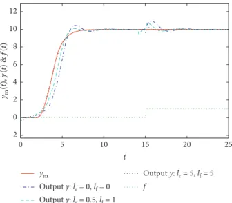
and selecting the sampling period to beT�0.1, the method in reference [18] is used for simulation. Figures 1 and 2 show the output response and tracking error when both the reference input signal and the fault signal are previewable, respectively.
The simulation results show that the effect of output tracking is noticeable under the preview compensations. By adopting the fault-tolerant preview control, the adverse effects caused by the fault signal can be effectively sup-pressed, and the response speed of the system output to the ideal value is accelerated.
If the fault signal is zero vector (i.e., no fault occurs), the controller designed here is still valid. Figures 3 and 4 reveal the output response and tracking error of the system in this case, respectively.
The simulation results illustrate that the tracking effect of the output vector of the original system to the ideal output vectors of the reference system is still noticeable under the action of reference input preview.
Example 2. Consider a fault-free system in the form of (1) with the following parameters [28, 29]:
E� 1 0 0 0 0 0 0 1 0 0 0 0 0 0 1 0 0 0 0 0 0 0 1 0 0 0 0 0 0 0 1 0 0 0 0 0 ⎡ ⎢ ⎢ ⎢ ⎢ ⎢ ⎢ ⎢ ⎢ ⎢ ⎢ ⎢ ⎢ ⎢ ⎢ ⎢ ⎢ ⎢ ⎢ ⎢ ⎢ ⎢ ⎢ ⎢ ⎢ ⎢ ⎢ ⎢ ⎢ ⎢ ⎢ ⎢ ⎢ ⎢ ⎢ ⎢ ⎢ ⎢ ⎢ ⎢ ⎢ ⎢ ⎢ ⎢ ⎢ ⎢ ⎢ ⎢ ⎢ ⎢ ⎢ ⎢ ⎢ ⎢ ⎢ ⎢ ⎢ ⎢ ⎢ ⎢ ⎢ ⎣ ⎤⎥⎥⎥⎥⎥⎥⎥⎥⎥ ⎥⎥⎥⎥⎥⎥⎥⎥ ⎥⎥⎥⎥⎥⎥⎥⎥ ⎥⎥⎥⎥⎥⎥⎥⎥ ⎥⎥⎥⎥⎥⎥⎥⎥ ⎥⎥⎥⎥⎥⎥⎥⎥ ⎥⎥⎥⎥⎥⎥⎥⎥ ⎥⎥⎥⎦ , A� 0 0 1 0 0 0 1 0 0 0 0 0 0 1 0 1 0 0 0 0 0 1 0 0 0 0 0 0 1 0 1 0 0 0 0 1 ⎡ ⎢ ⎢ ⎢ ⎢ ⎢ ⎢ ⎢ ⎢ ⎢ ⎢ ⎢ ⎢ ⎢ ⎢ ⎢ ⎢ ⎢ ⎢ ⎢ ⎢ ⎢ ⎢ ⎢ ⎢ ⎢ ⎢ ⎢ ⎢ ⎢ ⎢ ⎢ ⎢ ⎢ ⎢ ⎢ ⎢ ⎢ ⎢ ⎢ ⎢ ⎢ ⎢ ⎢ ⎢ ⎢ ⎢ ⎢ ⎢ ⎢ ⎢ ⎢ ⎢ ⎢ ⎢ ⎢ ⎢ ⎢ ⎢ ⎢ ⎢ ⎣ ⎤⎥⎥⎥⎥⎥⎥⎥⎥⎥ ⎥⎥⎥⎥⎥⎥⎥⎥ ⎥⎥⎥⎥⎥⎥⎥⎥ ⎥⎥⎥⎥⎥⎥⎥⎥ ⎥⎥⎥⎥⎥⎥⎥⎥ ⎥⎥⎥⎥⎥⎥⎥⎥ ⎥⎥⎥⎥⎥⎥⎥⎥ ⎥⎥⎥⎦ , B� 1 0 0 0 0 0 0 0 1 1 0 0 ⎡ ⎢ ⎢ ⎢ ⎢ ⎢ ⎢ ⎢ ⎢ ⎢ ⎢ ⎢ ⎢ ⎢ ⎢ ⎢ ⎢ ⎢ ⎢ ⎢ ⎢ ⎢ ⎢ ⎢ ⎢ ⎢ ⎢ ⎢ ⎢ ⎢ ⎢ ⎢ ⎢ ⎢ ⎢ ⎢ ⎢ ⎢ ⎢ ⎢ ⎢ ⎢ ⎢ ⎢ ⎢ ⎢ ⎢ ⎢ ⎢ ⎢ ⎢ ⎢ ⎢ ⎢ ⎢ ⎢ ⎢ ⎢ ⎢ ⎢ ⎢ ⎣ ⎤⎥⎥⎥⎥⎥⎥⎥⎥⎥ ⎥⎥⎥⎥⎥⎥⎥⎥ ⎥⎥⎥⎥⎥⎥⎥⎥ ⎥⎥⎥⎥⎥⎥⎥⎥ ⎥⎥⎥⎥⎥⎥⎥⎥ ⎥⎥⎥⎥⎥⎥⎥⎥ ⎥⎥⎥⎥⎥⎥⎥⎥ ⎥⎥⎥⎦ , C� 0 1 0 0 0 0 0 0 0 1 0 0 0 0 0 0 0 1 ⎡ ⎢ ⎢ ⎢ ⎢ ⎢ ⎢ ⎢ ⎢ ⎢ ⎢ ⎢ ⎢ ⎢ ⎣ ⎤⎥⎥⎥⎥⎥⎥⎥⎥⎥⎥⎥⎥⎥⎦. (61)
The system has impulse behavior and is impulse controllable.
Suppose the parameters in the reference model (2) are the same as Example 1 except
Cm� 1 0 0 1 0 0 ⎡ ⎢ ⎢ ⎢ ⎢ ⎢ ⎢ ⎢ ⎢ ⎢ ⎢ ⎢ ⎢ ⎢ ⎣ ⎤⎥⎥⎥⎥⎥⎥⎥⎥⎥⎥⎥⎥⎥⎦, (62)
and we can turn the model following problem into a stability problem by choosingxm(0) �0 0T,um(t)≡0. Let u(0) �0 0T, x(0) �5 5 5 5 5 5T, K� 0 0 0 −1 0 0 0 0 0 0 0 1 , Qe�10, Qx�10, R�1, lr�0. (63)
ym ( t ), y ( t ) & f ( t ) ym Output y: lr = 0, lf = 0 Output y: lr = 0.5, lf = 1 Output y: lr = 5, lf = 5 f −2 0 2 4 6 8 10 12 5 10 15 20 25 0 t
Figure1: Closed-loop output response with reference input preview and fault signal preview.
Tracking error e: lr = 0, lf = 0 Tracking error e: lr = 0.5, lf = 1 Tracking error e: lr = 5, lf = 5 –5 –4 –3 –2 –1 0 1 2 e ( t ) 5 10 15 20 25 0 t
Figure2: Output tracking error with reference input preview and fault signal preview.
ym ( t ) & y ( t ) –2 0 2 4 6 8 10 12 5 10 15 20 25 0 t ym Output y: lr = 0 Output y: lr = 0.5 Output y: lr = 5
Figure 5 shows the vector componentx1(t)drawn based on the methods of this paper and references [28, 29]. It can be seen that the control method in this paper can reduce overshoot and accelerate the system response.
7. Conclusion
In this paper, the controller design problem of impulse controllable descriptor systems with sensor failure is studied through the combination of model following control theory and preview control theory. Key features of the proposed method are summarized as follows: (i) the preview control theory is applied to the tolerant control, and the fault-tolerant preview controller improves the transient response of the closed-loop system; (ii) the impulse elimination and
the transformation for the quadratic performance index function are carried out for the more general descriptor systems based on reference [23], which is an extension of reference [10]. Our future research topics will focus on the fault-tolerant adaptive preview controller design for the hybrid systems based on references [30, 31].
Data Availability
Data sharing is not applicable to this article as no data sets were generated or analysed during the current study.
Conflicts of Interest
The authors declare that they have no conflicts of interest.
Acknowledgments
This work was supported by the National Key R&D Program of China (2017YFF0207401), innovative talents training fund of University of Science and Technology Beijing, and the Oriented Award Foundation for Science and Techno-logical Innovation, Inner Mongolia Autonomous Region, China (no. 2012).
References
[1] D. Cobb, “Feedback and pole placement in descriptor variable systems,” International Journal of Control, vol. 33, no. 6, pp. 1135–1146, 1981.
[2] G. Duan and A. Wu, “Impulse elimination via state feedback in descriptor systems,”Dynamics of Continuous, Discrete and Impulsive Systems, vol. 13, no. 1, pp. 722–729, 2006. [3] V. Lovass-Nagy, D. L. Powers, and R. J. Schilling, “On
reg-ularizing descriptor systems by output feedback,” IEEE Transactions on Automatic Control, vol. 39, no. 7, pp. 1507– 1509, 1994.
[4] L. Dai, “Impulsive modes and causality in singular systems,” International Journal of Control, vol. 50, no. 4, pp. 1267–1281, 1989.
[5] D. Chu and D. Cai, “Regularization of singular systems by output feedback,” Journal of Computational Mathematics, vol. 18, no. 1, pp. 43–60, 2000.
[6] C. Lin, J. Wang, D. Wang, and C. B. Soh, “Robustness of uncertain descriptor systems,” Systems and Control Letters, vol. 31, no. 3, pp. 129–138, 1997.
[7] D. Wang and P. Bao, “Robust impulse control of uncertain singular systems by decentralized output feedback,” IEEE Transactions on Automatic Control, vol. 45, no. 4, pp. 795– 800, 2000.
[8] T. Tsuchiya and T. Egami, Digital Preview and Predictive Control, Beijing Science and Technology Press, Beijing, China, 1994.
[9] M. Tomizuka and D. E. Rosenthal, “On the optimal digital state vector feedback controller with integral and preview actions,” Journal of Dynamic Systems, Measurement, and Control, vol. 101, no. 2, pp. 172–178, 1979.
[10] F. Liao, Y. Y. Tang, H. Liu, and Y. Wang, “Design of an optimal preview controller for continuous-times systems,” International Journal of Wavelets, Multiresolution and In-formation Processing, vol. 9, no. 4, pp. 655–673, 2011.
Tracking error e: lr = 0 Tracking error e: lr = 0.5 Tracking error e: lr = 5 5 10 15 20 25 0 t –5 –4 –3 –2 –1 0 1 2 e ( t )
Figure4: Output tracking error with reference input preview and
no fault occurs. x1 ( t ) a b c –2 0 2 4 6 1 2 3 4 5 6 7 8 9 10 0 t
Figure5: Response of the vector componentx1(t)under different
[11] A. Kojima and S. Ishijima, “.H∞ performance of preview control systems,”Automatica, vol. 39, no. 4, pp. 693–701, 2003.
[12] K. Takaba, “Robust preview tracking control for polytopic uncertain systems,” inProceedings of the 37th IEEE Conference on Decision and Control (Cat. No. 98CH36171), vol. 2, pp. 1765–1770, Tampa, FL, USA, December 1998.
[13] F. Liao, Y. Zhang, and Z. Gu, “Design of optimal preview controller for a class of linear discrete singular systems,” Control Engineering of China, vol. 16, no. 3, pp. 299–303, 2009. [14] F. Liao, Z. Ren, M. Tomizuka, and J. Wu, “Preview control for impulse-free continuous-time descriptor systems,” In-ternational Journal of Control, vol. 88, no. 6, pp. 1142–1149, 2015.
[15] M. Cao and F. Liao, “Design of an optimal preview controller for linear discrete-time descriptor systems with state delay,” International Journal of Systems Science, vol. 46, no. 5, pp. 932–943, 2015.
[16] Y. Lu, F. Liao, J. Deng, and C. Pattinson, “Cooperative optimal preview tracking for linear descriptor multi-agent systems,” Journal of the Franklin Institute, vol. 356, no. 2, pp. 908–934, 2019.
[17] B. Marx, D. Koenig, and D. Georges, “Robust fault-tolerant control for descriptor systems,”IEEE Transactions on Auto-matic Control, vol. 49, no. 10, pp. 1869–1875, 2004. [18] F. Shi and R. J. Patton, “Fault estimation and active fault
tolerant control for linear parameter varying descriptor sys-tems,”International Journal of Robust and Nonlinear Control, vol. 25, no. 5, pp. 689–706, 2015.
[19] Z. Wang, M. Rodrigues, D. Theilliol, and Y. Shen, “Actuator fault estimation observer design for discrete-time linear pa-rameter-varying descriptor systems,”International Journal of Adaptive Control and Signal Processing, vol. 29, no. 2, pp. 242–258, 2015.
[20] D. Kharrat, H. Gassara, A. E. Hajjaji, and M. Chaabane, “Adaptive observer and fault tolerant control for takagi-sugeno descriptor nonlinear systems with sensor and actuator faults,” International Journal of Control, Automation and Systems, vol. 16, no. 3, pp. 972–982, 2018.
[21] K. Han and J. Feng, “Data-driven robust fault tolerant linear quadratic preview control of discrete-time linear systems with completely unknown dynamics,” International Journal of Control, p. 11, 2019.
[22] D. Yang, Q. Zhang, B. Yao et al.,Singular Systems, Science Press, Beijing, China, 2004.
[23] F. Liao, C. Jia, U. Malik, X. Yu, and J. Deng, “The preview control of a class of linear systems and its application in the fault-tolerant control theory,”International Journal of Systems Science, vol. 50, no. 5, pp. 1017–1027, 2019.
[24] T. Katayama and T. Hirono, “Design of an optimal servo-mechanism with preview action and its dual problem,” In-ternational Journal of Control, vol. 45, no. 2, pp. 407–420, 1987.
[25] Q. Huang, J. Qin, A. Liang, and H. Li,Practical Technology for Steel Rolling Production, Metallurgical Industry Press, Beijing, China, 2004.
[26] G. Duan,Analysis and Design of Descriptor Linear Systems, Springer, New York, NY, USA, 2010.
[27] C. T. Chen,Linear System Theory and Design, Oxford Uni-versity Press, New York, NY, USA, 3rd edition, 1999. [28] B. Zhang, “Eigenstructure assignment for linear descriptor
systems via output feedback,”Asian Journal of Control, vol. 21, no. 2, pp. 759–769, 2019.
[29] G. Duan and R. J. Patton, “Eigenstructure assignment in descriptor systems via proportional plus derivative state feedback,” International Journal of Control, vol. 68, no. 5, pp. 1147–1162, 1997.
[30] K. Sun, S. Mou, J. Qiu, T. Wang, and H. Gao, “Adaptive fuzzy control for nontriangular structural stochastic switched nonlinear systems with full state constraints,”IEEE Trans-actions on Fuzzy Systems, vol. 27, no. 8, pp. 1587–1601, 2019. [31] J. Qiu, K. Sun, I. J. Rudas, and H. Gao, “Command filter-based adaptive NN control for MIMO nonlinear systems with full-state constraints and actuator hysteresis,”IEEE Transactions on Cybernetics, 11 pages, 2019.
Hindawi www.hindawi.com Volume 2018
Mathematics
Journal of Hindawi www.hindawi.com Volume 2018 Mathematical Problems in Engineering Applied Mathematics Hindawi www.hindawi.com Volume 2018Probability and Statistics
Hindawi
www.hindawi.com Volume 2018
Hindawi
www.hindawi.com Volume 2018
Mathematical PhysicsAdvances in
Complex Analysis
Journal ofHindawi www.hindawi.com Volume 2018
Optimization
Journal of Hindawi www.hindawi.com Volume 2018 Hindawi www.hindawi.com Volume 2018 Engineering Mathematics International Journal of Hindawi www.hindawi.com Volume 2018 Operations Research Journal of Hindawi www.hindawi.com Volume 2018Function Spaces
Abstract and Applied Analysis Hindawi www.hindawi.com Volume 2018 International Journal of Mathematics and Mathematical Sciences Hindawi www.hindawi.com Volume 2018Hindawi Publishing Corporation
http://www.hindawi.com Volume 2013 Hindawi www.hindawi.com
World Journal
Volume 2018 Hindawiwww.hindawi.com Volume 2018Volume 2018
Numerical Analysis
Numerical Analysis
Numerical Analysis
Numerical Analysis
Numerical Analysis
Numerical Analysis
Numerical Analysis
Numerical Analysis
Numerical Analysis
Numerical Analysis
Numerical Analysis
Numerical Analysis
Advances inAdvances in Discrete Dynamics in Nature and SocietyHindawi www.hindawi.com Volume 2018 Hindawi www.hindawi.com Differential Equations International Journal of Volume 2018 Hindawi www.hindawi.com Volume 2018