Diagnostic in Poisson Regression Models

 

© 2012 Università del Salento –  http://siba-ese.unile.it/index.php/ejasa/index

DIAGNOSTIC IN POISSON REGRESSION MODELS

Zakariya Y. Algamal

*

(1)_{Department of Statistics and Informatics, Mosul university, Iraq} Received 08 March 2011; Accepted 02 April 2012

Available online 14 October 2012

Abstract: Poisson regression model is one of the most frequently used statistical methods as a standard method of data analysis in many fields. Our focus in this paper is on the identification of outliers, we mainly discuss the deviance and Pearson χ2 as diagnostic statistics in identification. Simulation and real data are presented to assess the performance of the diagnostic statistics.

Keywords: Poisson regression, deviance, Pearson χ2, outliers.

1.

Introduction

Poisson regression models have received much attention in econometrics and medicine literature as model for describing count data that assume integer values corresponding to the number of events occurring in a given interval. The Poisson regression model is the most basic model, where the mean of the distribution is a function of the explanatory variables. This model has the defining characteristic that the conditional mean of the outcome is equal to the conditional variance [5]. Outliers are observations that do not follow the statistical distribution of the majority of the data. Outlier detection is a primary step in regression analysis and has attracted enormous attention in the literature over many years including Cook and Weisberg (1982), and Rousseeuw and Leroy (1987). There are a number of different statistics used by statistician to ordinary least squares regression. Leverage in Poisson regression is assessed by the hat values

i

h

.

DFBETA

and

DFFIT

are helpful for detecting influence in Poisson regression.

DFBETA

is calculated by finding the difference in an estimate before and after a particular

observation is removed. The same in

DFFIT

except the calculating difference will be in

predicted values.

The deviance plays an important role in assessing the fit of the model and statistical tests for parameters in the model, and also provides one method for calculating residuals that can be used

for detecting outliers [4]. Guria and Roy (2008) used the deviance for detecting outliers in logistic regression. Our focus in this paper is on the identification of outliers, we mainly discuss

the deviance and Pearson χ2 _{as diagnostic statistics in identification. The structure of the paper is}

the following. We briefly present in section 2 the estimation of the Poisson regression parameters for both deleted and undeleted observation. In section 3, we introduced the deviance and Pearson

χ2 criteria to detect the outliers. Simulation and real data examples are covered in section 4 and 5

respectively. Section 6 shows the conclusion.

2.

Background and Notation for the Poisson Regression Models

In Poisson regression model, hereafter PR, the number of events

y

has a Poisson distribution

with a conditional mean that depends on individual characteristics according to the structural model: ) x ( Exp ) x y ( E _{i i i} i = = ʹ′β θ (1)

Taking the exponential of

x

β

forces the expected count

µ

to be positive, which is required for

the Poisson distribution [5]. If a discrete random variable

y

follows the Poisson distribution,

then: ,.... 2 , 1 , 0 y , ! y e ) y Y ( p = = θy = θ − (2)

In order to estimate the PR estimator, we use the maximum likelihood estimation. By taking the

log-likelihood with θ_i =Exp(xʹ′_iβ), we get:

∑

= β = = β n 1 i i i i n 2 1 n 2 1,y ,...,y ,x ,x ,...,x ) logp(Y y ,x ) y ( L log (3)

{

}

∑

= − β ʹ′ + β ʹ′ − = β n 1 i i i i i ) y (x ) log(y !) x ( Exp ) ( L log (4)

The maximum likelihood estimator is then defined as:

) ( L log max arg ˆ_{ML= β} β _β (5)

So, the maximizing value for

β

is found by computing the first derivative of the (4) and setting

[

y Exp(x )

]

x 0 ) ( L log i n 1 i i i = β ʹ′ − = β ∂ β ∂

∑

= (6)

The second derivatives, Hessian matrix, is given below:

i i n 1 i i 2 x x ) x ( Exp ) ( L log ʹ′ β ʹ′ − = βʹ′ ∂ β ∂ β ∂

∑

= (7)

Since the equation (6) is nonlinear in

β

, one must use an iterative algorithm. A common choice

that work well is the Newton-Raphson method as: ML (m+1)

β

= ML (m)

β

−(

H

(m))−1 (m)

S

(8)

Where S is the first derivative of the log-likelihood [10],[11]. To see the influence of the deletion

of the kth observation on the PR, we consider the log-likelihood function as following:

{

}

∑

≠ = − β ʹ′ + β ʹ′ − = β n k , 1 i i i i i k Exp(x ) y (x ) log(y !) ) ( L log (9) then

[

]

i n k , 1 i i i ) k ( _{y Exp(x ) x} S

∑

≠ = β ʹ′ − = (10) x x ) x ( Exp _i n k , 1 i i ) k (

H

=−

∑

ʹ′β ʹ′ ≠ = (11)

Starting with an initial solution then the Newton-Raphson become:

S

H

(k) 1 (k) ) k )( m ( ML ) k )( 1 m ( ML ( ) − + − =

β

β

(12)

3.

Single Case Deletion Diagnostic

To show the amount of change in PR estimates that would occurred if the kth _{observation is}

deleted. Two diagnostic statistics are proposed, change in deviance and change in Pearson χ2 to

detect the outliers. Such diagnostic statistics are one that examine the effected of deleting single

case on the overall summary measures of fit. Let χ2_p denotes the Pearson χ2 statistics and χ2_p(k)

Pregibon (1981) [7] , it can be shown that the decrease in the value of the χ2_p statistic due to

deletion of the kth case is:

n

,...,

3

,

2

,

1

k

,

) k ( 2 p 2 p ) k ( 2 p

=

−

=

Δ

χ χ χ − (13) The χ2_p is defined as [6]: ) ˆ var( / )) x ( Exp y ( 2 n 1 i i i 2 p=

∑

− ʹ′β µ

χ

= (14)

And the χ2_p for the

k

th deleted case is:

) ˆ var( / )) x ( Exp y ( 2 n k , 1 i i i ) k ( 2 p =

∑

− ʹ′β µ

χ

≠ = − (15)

The one-step linear approximation for change in deviance when the kth case is deleted is:

) k ( ) k (

D

D

D

=

−

−

Δ

(16)

Because the deviance is used to measure the goodness of fit of a model, a substantial decrease in

the deviance after the deletion of the kth observation is indicate that is observation is a misfit.

The deviance of the PR model with and without the kth observation is respectively [4]:

)} ˆ y ( ) ˆ y ( log y { 2 D n _{i i} 1 i i i i − −µ µ =

∑

= (17) where µˆ_i =Exp(x_iʹ′βˆ): )} ˆ y ( ) ˆ y ( log y { 2 D n _{i i}( k) k , 1 i i( k) i i ) k ( − ≠ = − µ − − µ =

∑

(18)

A large value of

Δ

D

(k) indicates that the kth observation is an outlier.

A simulation study was conducted to investigate the behavior of the deviance and chi-square Pearson diagnostic statistics under various modeling scenarios. We considered data simulated

from a PR with sample size n and p explanatory variables for the cases (n,p)=(10,1),(25,2) and

(50,2). The first case represents a simple PR with X following uniform [0,1] distribution and

β=(0,1). The second and third case represent a multiple PR with

x

₁

and

x

₂ have uniform [0,1]

distribution and β=(0,1). The percentage of contamination was set to be 10%, 4% and 4%

respectively in order to make one or two observations from the response variable sever from

shift-mean outlier (the 10th observation from the first case, the 25th observation from the second

case, and observations 29 and 48 from the third case). For brevity, the

Δ

D

(k) and

Δ

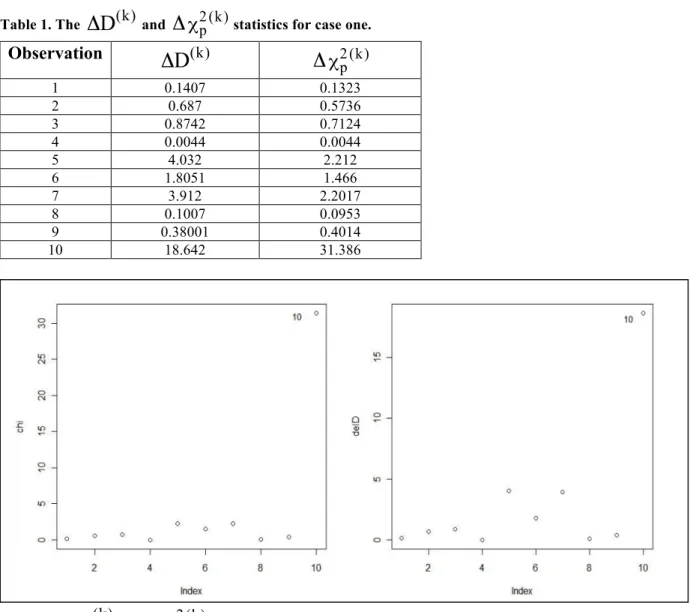
χ2_p(k) are

presented only in summary in table 1 for the first case, while the rest case results are shown in figure 2 and figure 3.

Table 1. The

Δ

D

(k) and

Δ

χ2_p(k) statistics for case one. Observation

D

(k)

Δ

Δ

χ2_p(k) 1 0.1407 0.1323 2 0.687 0.5736 3 0.8742 0.7124 4 0.0044 0.0044 5 4.032 2.212 6 1.8051 1.466 7 3.912 2.2017 8 0.1007 0.0953 9 0.38001 0.4014 10 18.642 31.386

Figure 1.

Δ

D

(k) and

Δ

_χ2_p(k) for the first case.

The deviance for the full model was (25.37). The 10th observation will be outlier since it has

642

.

18

D

(k)

=

Δ

and

Δ

χ2_p(k)

=

31

.

386

. Figure 1 shows the

Δ

D

(k) and

Δ

χ2p(k) for this case.  

 

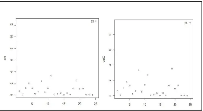
  Figure 2.

Δ

D

(k) and

Δ

_χ2_p(k) for the second case.

From figure (2) we can conclude that the observation 25 will be outlier since its deletion will

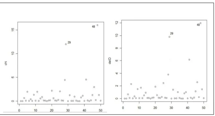
decrease the deviance and Pearson χ2 by (10.3) and (13.4). Again from figure (3), we can

considered observations 29 and 48 are outliers since they have large

Δ

D

and

Δ

χ2_p among the

Figure 3.

Δ

D

(k) and

Δ

_χ2_p(k) for the third case.

5.

Numerical Results

The performance of the delta deviance and delta Pearson χ2 diagnostic statistics was studied in a

real data example. Andersen (2008) [1] described data for Canadian Equality, Security, and

Community Survey of 2000. He used only Quebec respondents in the analysis where (n=949).

The response variable is the number of voluntary associations to which respondents belonged. The explanatory variables are gender (with women as the reference category), Canadian born (the reference category is "not born in Canada"), and language spoken in the home (divided into English, French, and other, with French coded as the reference category). He used Cook's distance which indicates that there are two observations (31 and 786) may be particularly

problematic. Also, he pointed that the analysis of the

DFBETA

indicates that the influence of

these two observations is largely with respect to the effect of Canadian born variable. To assess

our diagnostic statistics performance, we used this example. Table (2) shows the

Δ

D

(k) and

χ

Δ

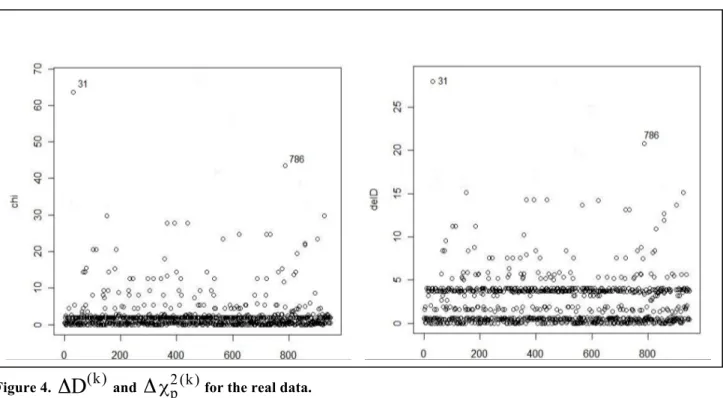
2p(k) only for the two observations (31 and 949), where the full model deviance is 2427.632.

Figure 4 shows the overall look about our analysis.

Table 2. The

Δ

D

(k) and

Δ

χ2_p(k) for the real data. Observation

D

(k)

Δ

Δ

χ2p(k)

31 28.00042 63.5904

786 20.813 43.595

  Figure 4.

Δ

D

(k) and

Δ

χ2_p(k) for the real data.

 

6.

Conclusion

All of the diagnostic statistics described in this paper use one-step approximations to measure the effect of single case deletion on the Poisson regression model parameters. As we can see from figure 1 that the observation 10 considered outlier by our diagnostics statistics and this corresponds the fact that case 10 has already sever from shifting in mean comparing with the rest observations. The same with observation 25 from figure 2 and observations 29 and 48 from figure 3.

As mentioned in section 5 and from figure 4, the observations 31 and 786 considered outliers

using delta deviance and delta Pearson χ2 diagnostic statistics, this is the same decision that made

by Andersen (2008) using

DFBETA

. It should be noted here that the DFFIT pointed out that

the observation 31 has the value 0.0114 which is less than the traditional cut-off value 0.129 and that the observation 786 has the value 0.312 which is greater than the traditional cut-off value. Here we could conclude that our diagnostic statistics well done in identifying outliers.

References

[1]. Andersen, R. (2008). Modern methods for robust regression. New York: SAGE

Publication.

[2]. Cook, R. D. and Weisberg, S. (1982). Residuals and influence in regression. New York:

Chapman & Hall.

[3]. Guria, S. and Roy, S. S. (2008). Diagnostics in logistic regression models. Journal of the

Korean Statistical Society, 37, 89-94.

[4]. Jong, P. and Heller, G. Z. (2009). Generalized linear models for insurance data. London: Cambridge University Press.

[5]. Long, J. S. (1997). Regression models for categorical and limited dependent variables.

New York: SAGE Publication.

[6]. McCullagh, P. and Nelder, J.A. (1989). Generalized linear models. 2nd ed. London:

Chapman & Hall.

[7]. Pregibon, D. (1981). Logistic regression diagnostics. The Annals of Statistics, 9, 4,

705-724.

[8]. Rousseeuw, P. J. and Leroy, A. M. (1987). Robust regression and outliers detection. New

York: John Wiley.

[9]. Seber, G. A. F. and Lee, A. J. (2003). Linear regression analysis. 2nd ed. New Jersey:

John Wiley.

[10]. Winkelmann, R. (2008). Econometric analysis of count data. 5th ed. Leipzing: Springer.

[11]. Yan, X. and Su, X. G. (2009). Linear regression analysis, theory and computing.