Finding and Tracking Multi-Density Clusters in
Online Dynamic Data Streams
Conor Fahy and Shengxiang Yang,
Senior Member, IEEE
,
Abstract—Change is one of the biggest challenges in dynamic stream mining. From a data-mining perspective, adaptingand tracking change is desirable in order to understand how and why change has occurred. Clustering, a form of unsupervised learning, can be used to identify the underlying patterns in a stream. Density-based clustering identifies clusters as areas of high density separated by areas of low density. This paper proposes a Multi-Density Stream Clustering (MDSC) algorithm to address these two problems; the multi-density problem and the problem of discovering and tracking changes in a dynamic stream. MDSC consists of two on-line components; discovered, labelled clusters and an outlier buffer. Incoming points are assigned to a live cluster or passed to the outlier buffer. New clusters are discovered in the buffer using an ant-inspired swarm intelligence approach. The newly discovered cluster is uniquely labelled and added to the set of live clusters. Processed data is subject to an ageing function and will disappear when it is no longer relevant. MDSC is shown to perform favourably to state-of-the-art peer stream-clustering algorithms on a range of real and synthetic data-streams. Experimental results suggest that MDSC can discover qualitatively useful patterns while being scalable and robust to noise.
Index Terms—Data stream clustering, multi-density clustering, concept drift, concept evolution, swarm intelligence, change detection
F
1
I
NTRODUCTIONA
NALYSING data-streams in real-time is a natural and necessary progression from traditional batch data-mining. Clustering data streams requires additional consid-erations to traditional clustering. As in all stream-mining tasks, speed and memory constraints exist; often only a single pass of the data is afforded and it is not practical to store all processed data. In non-stationary streams changeis a further consideration. A stream-clustering algorithm should be able to detect and adapt to change. Ideally, this change would be tracked and a ‘narrative’ could be inferred from the pattern-changes over time. Furthermore, by understanding and tracking the underlying patters, we can identifydeviationsfrom these patterns - an indication of change or anomaly.
Change in a stream can happen in a number of ways; Let S = [xt]∞
t=0 denote a stream where xis a vector in d dimensions at timet. LetY represent the set ofkdiscovered clusters:Y ={y1, . . . , yk}. We can represent the assignment of a pointxito a clusteryj ∈Y over time as a conditional probabilityPt(y
j|xi); the probability of xi belonging to a cluster yj at timet. One possible change in a data-stream can occur in the form of concept drift. This occurs if the characteristics of the data change, i.e., if the underlying process generatingxchanges. For example, sampling from source distribution Cj decreases and sampling fromCj+1 increases. Typically, this kind of drift is referred to as virtual drift, a change inP(x). A second type of drift is known as real drift: a change inP(y|x). For example, at timetpointxi is assigned to clusteryj, but att+δ,xiis assigned to cluster
Manuscript received 4 September, 2018; Revised 13 January, 2019 and 22 March, 2019; accepted 5 May 2019. (Corresponding author: Shengxiang Yang)
The authors are with the Centre for Computational Intelligence (CCI), School of Computer Science and Informatics, De Montfort University, The Gateway, Leicester LE1 9BH, U.K. (email:{conor.fahy, syang}@dmu.ac.uk).
ym. This would occur, in this example, if clustersyjandym have drifted into different positions in the feature space.
Another possible change is concept evolution. Concept evolution occurs when an entirely new cluster ym, i.e., ym 6∈ Y, appears in the stream. Assuming a fixed k can lead to a poorer clustering performance. Concept evolution is a particular challenge as it relates to one of the most fundamental questions in clustering - how many clusters are present in the data? This is difficult in dynamic environ-ments as this number will change over time. Density based clustering methods can discover the natural clusters in data without requiring their number to be specified a-priori.
Density based methods identify clusters as areas of the feature space with high density separated by areas of low density. Dense areas are described using micro-clusters. A micro-cluster is ad-dimensional sphere with a centrecand a radiusr. Micro-clusters have a maximum radius of, where r ≤. A data point is assigned to a micro-cluster if it falls within the area of the micro-cluster. The set of micro-clusters that are connected form the macro-cluster. This allows for arbitrarily shaped clusters to discover dense areas of the feature space.
The maximum radius permitted for each micro-cluster, the-neighbourhood, defines the concept of ‘dense’. This is a sensitive parameter; if it is too large, multiple concepts will be clustered as one. If too small, no clusters will form at all. Furthermore, if this parameter is global, i.e., each cluster is constrained by the same value of , then performance will degrade when the stream contains clusters of varying densities. As an example, a Gaussian source distribution that generates n points with a low variance will be more ‘dense’ than the same process with a large variance. A global imposes limitations on the type of clusters that can be discovered. For example, embedded or overlapping clusters will be missed if only using a single concept of density.
Recent proposals to capture multi-density clusters [3], [10] in a data-stream (and clustering data streams in general [6], [13], [18]) rely on a number of sensitive user-defined parameters. The values of these parameters greatly affect the clustering performance and not much consideration is given to their practicality in a non-stationary environment. For example, how should these parameters be tuned? If we follow traditional methods, we could use a portion of the stream as a test set and use this to find the best set of parameters. However, in a dynamic environment, it is likely that the best values for these parameters will change over time.
Motivated by these challenges, we propose a Multi Density Stream Clustering (MDSC) algorithm. In MDSC, clusters are discovered with an adaptive , local to each cluster. Each newly incoming data point is treated as a single micro-cluster which attempts to merge with existing, live clusters. If the micro-cluster can not merge with an already discovered cluster, it attempts to merge with a micro-cluster in the outlier buffer. Otherwise, it joins the buffer as a new micro-cluster. This buffer is checked periodically for new clusters. A micro-cluster will age if no new data is added and it will eventually disappear if it is no longer relevant. This mechanism of ageing micro-clusters and an outlier buffer allows concept drift to be tracked and noise to be effectively treated. The interval at which the buffer is checked and the rate at which micro-clusters age are determined by a single user-defined parameter. A second user-defined parameter determines the age at which micro-clusters are considered no longer relevant and removed. These are the only user parameters and their values will depend on the velocity of the stream and the granularity the user wishes to examine it.
A swarm intelligence approach is used to discover new clusters in the buffer. The process is inspired by the nest-building behaviour of certain species of ant. Micro-clusters form ‘nests’ with similar micro-clusters. The similarity be-tween each nest is estimated in an iterative, decentralised way, similar to the collective memory of an ant colony in the form of pheromone trails. Clusters are formed based on these nests and their similarity. We use an ant-inspired swarm-intelligence, as opposed to other swarm intelligence approaches (for example fire-fly [40], PSO [31], or artificial bee-colony [23]) because of this path-building ‘memory’ mechanism in the form of pheromone trails.
In summary, the main contributions of this paper are: • The parameter in MDSC is adaptive and local to
each cluster allowing for the discovery of clusters with varying densities.
• Discovered clusters are maintained online and la-belled in order to track changes. Streams can be anal-ysed in real time or at higher levels of granularity. The rest of the paper is organised as follows: Section 2 provides an overview of related work in the literature. Section 3 presents our proposed algorithm in detail. Section 4 outlines our experimental set-up. An analysis on the algorithm’s scalability and robustness to noise is reported in Section 6, a sensitivity analysis in Section 7 and an analysis of the time and space requirements is presented in Section
8. Discussion and conclusions are offered in Sections 9 and 10, respectively.
2
R
ELATEDW
ORKStream-clustering algorithms typically adopt the two-phase online/offline approach proposed inCluStream[1]. The au-thors suggest that a stream clustering algorithm could con-sist of an on-line phase which summarises the data and an off-line phase which clusters the summaries. CluStream in-troduced the concept of the micro-cluster to summarise the data. A micro-cluster is a temporal extension to the cluster-feature vector proposed in BIRCH [38]. In CluStream, data is summarised online and the offline clustering of the micro-clusters is based on the k-means algorithm [17]. Density based methods have been extended for data-streams using the two-phase approach [13], [6], [34], [35]. Density based clustering [11] is an attractive method for clustering data streams because it is robust to noise, the number of clusters does not have to be specified a-priori, and arbitrarily shaped clusters can be discovered - as opposed to hyper-elliptical shapes as in k-means and its variants.
MR-Stream[35] partitions the search space into discrete cells and uses a tree structure to store this space partitioning. New data points are assigned to a cell and the tree structure is updated on-line. The off-line clustering is performed on the summarised tree.ClusTree[24] also uses a tree structure to maintain summaries of the data stream and the sum-maries are clustered using the k-means algorithm. Similar to MR-Stream,D-Stream[34] partitions the search space into discrete grid sections. Newly arriving data is mapped onto a grid and then clustered offline.
DenStream [6] is a popular stream clustering algorithm and widely used as a benchmark [3], [13], [15]. Data points are read online and summarised as micro-clusters. Den-Stream uses the time-dampened window model to give higher weights to recent data and when a clustering request is made by a user, these micro-clusters are clustered off-line using a traditional density-based clustering algorithm [11]. However, as noted in [15], the off-line clustering is computationally expensive and, furthermore, the off-line clustering only happens at the request of the user. This presents a dilemma because frequent requests could better discover changes in the stream but they are costly. Infre-quent requests are less costly but could potentially miss changes in the stream. Efforts have been made to address this problem by merging the on-line and off-line phases into a single on-line phase inCEDAS[18],FlockStream[15],
SOStream[20] andSVStream[36].
CEDAS[18] uses a graph structure to store the relation-ship between on-line micro-clusters, micro-clusters act as nodes in a graph and their edges form the the macro-cluster. Micro-clusters are either an outlier or part of a cluster and all are time-weighted. A micro-cluster has an ‘energy’ level and if it is not updated, it loses this energy until it is considered no longer relevant and is removed. SOStream is based on DBSCAN [11] and self-organising maps while SVStream [36] is based on the one-class support vector do-main description classification method [33].FlockStream[15] is a bio-inspired swarm intelligence approach which also combines the online/offline approach into a single online
phase. FlockStream is modelled on the flocking behaviour of birds as proposed in Reynolds’ Boids [29].There are many more techniques for density clustering that are similar to the ones described here and a comprehensive review of density based stream clustering is given in [4]. A common shortcoming among all of these algorithms is their inability to detect clusters of varying densities.
The reason for this restriction to a single concept of density is the use of global parameters for each cluster. Algorithms which use micro-clusters as the summarisation mechanism [6], [13], [15] define the micro-cluster parameters globally. The-neighbourhood defines the maximum radius for a micro-cluster and the minPoints parameter defines how many points a micro-cluster must contain before it can be defined as ‘dense’. These parameters apply to every discovered cluster. Solutions have been proposed to the multi-density problems in stationary batch data. Most are extensions of the DBSCAN algorithm [11]. However, these algorithms are not suitable for data streams because they require more than a single pass of the data or require prohibitively high computational time.
Methods for discovering multi-density clusters in streams have been proposed in MuDi [3] and ADStream
[10]. Both combine a density-based and grid-based approach to clustering data streams. They use the two phase on-line/offline approach. MuDi proposes a further extension to DBSCAN called M-DBSACN which is used to form multi-density clusters. ADStream uses a combination of multi-density clustering and affinity propagation clustering [16] to find clusters off-line based on the data mapped to the grid. Among other parameters, the size of each grid is an im-portant consideration as it defines the concept of ‘dense’. In each of these algorithms it is a sensitive, global user-defined parameter.
We previously proposed Ant Colony Stream Clustering (ACSC) [13], a swarm inspired clustering method. ACSC extends some of the fundamental micro-cluster concepts introduced in Denstream [6]. These micro-clusters are con-sidered as ‘ants’ which self-organise to form ‘nests’ with similar ants. Established nests form the macro-cluster. It uses the two-phase approach which makes it impossible to automatically track clusters and furthermore, it was re-stricted to finding clusters of a single level of density. We further proposed ACMDSC [14] as a potential method to discover multi-density clusters but this method also relies on the two phase approach and requires sensitive, static parameters. The proposed approach in this paper builds on the same DenStream fundamentals (outlined in the Section 3, Preliminaries) and uses some of the same concepts as ACSC (ants, nests , and pheromone trails) but outlines a novel clustering mechanism in order to cope with multi-density clusters in an on-line setting.
In summary, density based clustering has advantages in that arbitrary shaped clusters can be discovered (as opposed to just hyper-spherical), the number of clusters does not have to specified a-priori and data can be compactly sum-marised as micro-clusters. The majority of density stream clustering methods adopt the two phase, on-line/off-line approach whereby data is first summarised online and then clustered offline (CluStream [1], ClusTree [24], DenStream [6], D-Stream [34], MR-Stream [35], ACSC [13], and others).
The disadvantages of this approach are that a) the behaviour of clusters cannot be tracked over time and b) only clusters of a single density can be discovered. Recently, MuDi [3] and AD-Stream [10] have been proposed to discover multi-density clusters in streaming data, however they require sensitive, static parameters and use the two phase approach. The two-phase approach has been combined into a sin-gle online phase (Flockstream [15], CEDAS [18], SOStream [20], SVStream [36]) potentially (with small algorithmic ex-tensions) allowing for on-line tracking, however they are unable to deal with multi-density clusters. The method proposed in this paper aims to fill the space here; an online method allowing multi-density clusters to be discovered and tracked over time.
3
P
ROPOSEDM
ULTI-D
ENSITYS
TREAMC
LUSTER-ING
(MDSC) A
LGORITHM3.1 Preliminaries
We introduce the fundamental micro-cluster concepts origi-nally proposed in [6] and extended in [15], [13], [14].
A micro-cluster containingNpoints{X~i},i={1, ..., N}, is described using four components: N, the number of points contained in the micro-cluster, each of which is ann -dimensional vector; LS, the linear sum of these points (i.e.,
N
P
i=1 ~
Xi); SS, the squared sum of these points (i.e., N
P
i=1 ~ Xi2); and a time stamp lastEdit. LS and SS are n-dimensional vectors. From the first three components, we can obtain the centrecand radiusrof the micro-cluster [1], as follows:
c=LS N (1) r= s SS N − LS N 2 (2) The fourth component,lastEdit, records the most recent time a micro-cluster was updated.
Micro-clusters are increment-able so at time T a point
pin d dimensions can be absorbed into an existing micro-clusterm: m.N += 1 m.LSi =m.LSi+pi,∀i∈ {1,2, ..., d} m.SSi=m.SSi+p2i,∀i∈ {1,2, ..., d} m.lastEdit=T (3)
wherepiis theithdimension of pointp. Two existing micro-clustersmiandmjcan merge into a new micro-clustermk,
iff rmk ≤, wherermkis the radius ofmk, as follows: mk = (Ni+Nj, ~LSi+LS~j, ~SSi+SS~j, T) (4) Two micro-clusters mi and mk are said to be density reachable if:
dist(cmi, cmk)≤ (5)
where cmi andcmk are the centres ofmi and mk,
respec-tively, anddist(cmi, cmk)is the Euclidean distance between cmiandcmk. ThelastEditcomponent is used to calculate the
micro-cluster’s age:
age=T−lastEdit (6)
3.2 Finding New Clusters in the Buffer
During the initialisation step of the algorithm,λpoints are collected in the buffer and the initial clusters are discovered. Any points not belonging to a cluster are retained in the buffer. Once the clusters are live, incoming data points are processed and those points which are not assigned to an existing cluster are passed to the outlier buffer. This buffer is periodically checked. Clusters are discovered in two steps in an ant-inspired, swarm intelligence approach; initially, micro-clusters form ‘nests’ with similar micro-clusters and subsequently, similar nests are grouped to form the cluster. 3.2.1 Finding Nests
The step begins with a list of all micro-clusters currently stored in the buffer and a program variable -init. An appropriate value foris discovered adaptively using-init
as an initial ‘starting point’.
In the biological metaphor, the micro-clusters are ants and a nest is a grouping of similar ants. Ants are iteratively assigned to nests representing dense areas of the data. The first ant creates the first nest and subsequent ants can either join an existing nest or form a new one.
Each ant visits each nest in succession and evaluates the nest’s suitability by comparing itself with all ants currently in the nest. Formally, the similarity of anta with nest k is defined as follows: Sim(a, k) = 1 nk nk X j=1 dist(a, kj) (7)
where nest k already has nk ants present in it (i.e., k = {k1, k2, ..., knk}). Antajoins the most similar nestprovided
its similarity score is equal to or below the initial value of -init (-init is a program variable). If not, it forms a new nest.
As an ant evaluates each nest, it ‘remembers’ its sim-ilarity with each nest (Eq. (7)). Upon joining a nest or establishing a new nest, the similarity of the selected nest with all its neighbouring nests is updated. This similarity update happens in a decentralised, iterative way, similar to pheromone trails in an ant colony and these similarity scores are recorded in a matrix, which is referred to as the Pheromone Matrix (PM). The pheromone trail to each neighbouring nest is a rolling average updated whenever a new ant joins the nest. Formally, the pheromone trail between nestsk and l is the average of each ant iin nest k’s similarity (Eq. (7)) with nestl:
ph(k, l) = 1 nk nk X i=1 Sim(ki, l) (8)
wherenk is the number of ants in nestkandki is thei-th ant in nestk.
Once all the ants have been assigned to their respective nests, the contents of each nest are merged into a single micro-cluster (Eq. (4)) withno restriction on maximum radius
(i.e., = 1). The pseudo-code for this step is presented in Algorithm 1. Micro-clusters formed in this stage will vary in size, both in terms of radius and number of points contained. At the end of the step we have n nests, each
Algorithm 1Create Nests
Input:List of micro-clusters in buffer, parameter-init
Output:Nests and Pheromone Matrix
1: for<each micro-cluster m>do 2: if<nests>then
3: for<each nest n>do
4: Calculate similarity ofmton(Eq. (7))
5: if<similarity ≥ >then
6: Addmton
7: Update pheromone trail (Eq. (8))
8: else if<No suitable nest>then 9: Create a new nest
10: Addmto the new nest
11: Initialise pheromone trail
12: for<each created nest n>do 13: Mergeninto single micro-cluster
14: returnNests, Pheromone Matrix
containing a single micro-cluster and a PM describing the similarity between each pair of nests as follows:
PM= N1 N2 . . . Nn 0 ph(N1, N2) . . . ph(N1, Nn) N1 ph(N2, N1) 0 . . . N2 .. . ... . .. ... . . . ph(Nn, N1) . . . 0 Nn (9) 3.2.2 Creating Clusters
The previous step summarised the buffer contents into a fewer number of heterogeneous micro-clusters, represented as a set of nests. In this step, clusters are discovered incre-mentally, starting with the most dense. This allows for the discovery of embedded and overlapping clusters.
A new clusterC is seeded with the densest nest in the set of nests as follows:
seed= max
k∈N ests(k.N) (10) Taking this nest as the initial nest,initNest, we find its closest neighbour,closestNest, in the pheromone matrix, as follows: We merge these two nests into a single nest, the seed
nest. ClusterC’s-value is taken as the radius of this seed nest. Intuitively, clusters which are more sparse will have a greater distance between the initial nest and its closest neighbour (and consequently a larger). Conversely, more compact clusters will have a shorter distance and a smaller .
Along with , cluster C requires an additional value,
threshold, in order to group similar, density reachable nests which remain in the buffer. This determines if a nest added toCis abordernest. A border nest is a nest which is density reachable to C but has a density (N) of less thanα times the density ofinitNest. For example, ifinitNestcontains 100 points andα= 0.1, a border nest will contain 10 or fewer points.T hresholdis local toCand relative to the density of C, controlled by a static program-variableα. Formally;
Algorithm 2Initialise Cluster
Input:Nests, Pheromone MatrixP M, Parameterα Output:ClusterC
1: Find the densest nestinitN estin Nests (Eq. (10))
2: initialDensity=initN est.N
3: FindinitN est’s closest neighbourclosestN est(Eq. (12))
4: MergeinitN estandclosestN estinto new micro-cluster seed
5: Initialse new clusterC:=seed 6: C.:=rseed
7: C.threshold:=initialDensity∗α
8: RemoveinitN estandclosestN estfrom Nests and PM
9: returnC
Border Nest
𝑁 ≤ 𝑖𝑛𝑖𝑡𝑁𝑒𝑠𝑡. 𝑁 ∗ α
initNest
Cluster C
Fig. 1: Illustrative example of clusterC in black. Although the red micro-cluster is density reachable toC, it is only via a border nest so does not become part ofC.
This seeding process is outlined in Algorithm 2.
Nests in the buffer which are density reachable to a border nest in C and not reachable to any other nest in C are not added to C. They remain in the buffer. This is illustrated in Fig. 1. This mechanism promotes the formation of homogeneous, pure clusters by preventing two (or more) similar concepts being clustered as one due to a small num-ber of intermediary points. Furthermore, because nests are formed starting with the most dense (and therefore smallest ), overlapping and embedded clusters can be discovered.
closestN est=max(P M[:, initN est]) (12)
Once all nests which are density reachable to C are identified, the overall size ofCis calculated - this is simply the number of data points described by C. If this size is greater than a minimum cluster size (proportionate to λ), C is added to the set of online clusters. If C contains fewer points than the minimum cluster size, the clustering operation is undone and the original micro-clusters remain in the buffer.
Before addingCto the set of online clusters, it is given a unique ID. This is a global parameterclusterNum, which is assigned to a cluster and then incremented, i.e., the first cluster is labelled as 1, the second as 2, and so on.
Outlier and noise points will unlikely ever get clustered and, because they are subject to an ageing process, they will eventually disappear in the buffer.
The pseudo-code for finding clusters from the initial nests is outlined in Algorithm 3.
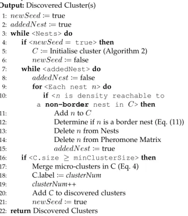
Algorithm 3Find Clusters
Input:Nests, Pheromone MatrixP M, parametersminClusterSize,clusterNum
Output:Discovered Cluster(s)
1: newSeed:=true
2: addedN est:=true
3: while<Nests>do
4: if<newSeed= true>then
5: C:=Initialise cluster (Algorithm 2)
6: newSeed:=false
7: while<addedNest>do 8: addedN est:=false
9: for<Each nest n>do
10: if <n is density reachable to a non-border nest in C>then
11: AddntoC
12: Determine ifnis a border nest (Eq. (11))
13: Deletenfrom Nests
14: Deletenfrom Pheromone Matrix
15: addedN est:=true
16: if<C.size ≥ minClusterSize>then 17: Merge micro-clusters in C (Eq. 4)
18: C.label:=clusterNum
19: clusterNum++
20: AddCto discovered clusters
21: newSeed:=true
22: returnDiscovered Clusters
3.3 Incoming Points
Online clusters are maintained as a set of connected micro-clusters. Each cluster has a unique id and a uniquevalue. A newly arriving pointpinddimensions is first converted to a micro-clustermas follows: m.N = 1 m.LSi=pi,∀i∈ {1,2, ..., d} m.SSi=pi2,∀i∈ {1,2, ..., d} m.lastEdit=T (13)
The incoming micro-cluster attempts to join an existing cluster, checking each one beginning with the most compact, i.e., the cluster with the smallest value. The new micro-cluster checks if it is density reachable (Eq. (5)) to any micro-cluster in the selected cluster. If so, it attempts to merge (Eq. (4)). If the merging operation is a success, the merged micro-cluster’s time-stamp is updated, otherwise, the newly-arrived micro-cluster is just added to the clus-ter (un-merged). If the newly arriving micro-clusclus-ter is not density reachable to any micro-cluster in any of the existing clusters, it is passed to the buffer. Here, it attempts to merge with a micro-cluster already present in the buffer, otherwise it joins the buffer as a new micro-cluster.
4
E
XPERIMENTALS
ETUPMDSC is evaluated in a number of ways. Initially, we evaluate MDSC’s performance on 4 real-data benchmark streams across three external metrics. We select 4 data-streams from different fields to examine the performance of the algorithm without any parameter tuning. We compare
the performance of MDSC with four peer density clustering algorithms. We then examine the algorithm’s performance with synthetic data-streams exhibiting concept drift, con-cept evolution and clusters with varying densities. Finally, we examine the qualitative performance of the discovered clusters on a data-stream we collected from an air-quality monitoring system in Leicester City, UK.
4.1 Peer Algorithms
MCSC is evaluated against four state-of-the-art peer algo-rithms; MuDi [3], CEDAS [18], DenStream [6] and ACSC [13]. Similar to MDSC, they each employ micro-clusters to identify dense areas of the stream. DenStream is one of the original density-based stream clsutering algorithms. Data is summarised online and clustered offline with DBSCAN [11]. ACSC is an ant-inspired approach using the tumbling window model. Clusters are discovered at fixed intervals. MuDi also finds clusters at fixed intervals, incoming points are assigned to a grid structure and when a grid’s density reaches a certain threshold, a micro-cluster is formed. These micro-clusters are clustered offline using an extension to DBSCAN which allows for the discovery of multi-density clusters. CEDAS uses a graph structure to find clusters, points are assigned to micro-clusters which act as nodes in a graph structure. Connected ‘nodes’ form the macro-cluster. 4.2 Data Sets
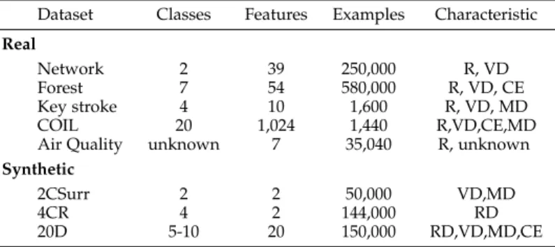
The performance of MDSC is compared to the peer algo-rithms across seven benchmark datasets. Though the data sets themselves are static, each point is read sequentially, simulating a stream. These streams are dynamic in that they exhibit concept drift and concept evolution. Three datasets are taken from the Non-Stationary Environment Archive used in [8] and made publicly available by the authors1.
Two of these datasets are synthetic and are composed of non-stationary 2-D Gaussian clusters.2CSurris composed of two clusters with different densities. One cluster is sta-tionary and the other is dynamic, exhibiting virtual concept drift (a change in P(x)). The other dataset, 4CR, consists of 4 clusters rotating anti-clockwise, an example of real virtual drift (a change in P(y|x)). The third dataset taken from this archive is a real-world problem based on the use of keystroke dynamics to recognise users by the natural pattern of their typing rhythm, which is likely to change over time. It is based on 4 different users typing a 10-key password 400 times. The 10 variables measure the flight-time between each key, i.e., the flight-time difference between a key being released and the next one being pressed, giving a total of 1,600 samples with 10 dimensions.
MDSC is also tested on the popular Network Intru-sion benchmark dataset used in [6], [13], [15], [18]. This dataset is composed of seven weeks of simulated network requests on the DARPA network. Requests can be ‘normal’ or ‘malicious’. The non-stationary ‘malicious’ class contains substantial drift as it is composed of 23 different types of attacks. The Forest Cover data-stream is another popular benchmarking data-stream. It is composed of 54 carto-graphic variables describing forest coverage in Roosevelt
1. https://sites.google.com/site/nonstationaryarchive/
TABLE 1: Description of datasets used in experiments. R = Real Data, VD = Virtual Drift, RD = Real Drift, MD = Multi-Density, CE = Concept Evolution
Dataset Classes Features Examples Characteristic
Real
Network 2 39 250,000 R, VD
Forest 7 54 580,000 R, VD, CE
Key stroke 4 10 1,600 R, VD, MD
COIL 20 1,024 1,440 R,VD,CE,MD
Air Quality unknown 7 35,040 R, unknown
Synthetic
2CSurr 2 2 50,000 VD,MD
4CR 4 2 144,000 RD
20D 5-10 20 150,000 RD,VD,MD,CE
National Forest of northern Colorado and is widely used in the stream-mining literature [1], [3], [24], [13] as it exhibits fairly rapid virtual drift. We also include a high-dimensional data-stream, COIL2. This is a dataset of 20 grey-scale images
in 1024 dimensions (32 by 32 pixels) and exhibits concept evolution.
In order to evaluate the performance of MDSC on a stream exhibiting all of the challenging stream character-istics: concept evolution, real drift, virtual drift and multi-density clusters, we generated a further synthetic data-stream with a dimensionality of 20. Clusters are Guassian and at periodic drift-intervals we shift the centre and the variance of each one to simulate drift and varying densities. At each drift interval, we randomly add or remove a cluster (within bounds) to simulate concept evolution. SynStream is a tool we developed to create this type of synthetic stream and we will offer this to the community for benchmarking and testing at due time.
A real-life stream is taken from UK-AIR database main-tained by the Department of Environment, Food and Rural Affairs (DEFRA)3. The data-stream is taken from a single
monitoring site in Leicester City and provides seven hourly air-quality measurements regarding Ozone (O3), Nitric Ox-ide (N O), Nitrogen Dioxide (N O2), Nitrogen Oxides (N Ox), Particulate Matter 2.5 (P M2.5), Non-volatile PM2.5 (P Mnv), and volatile PM2.5 (P Mv). These seven pollutants are mea-sured in micrograms (one-millionth of a gram) per cubic meter air orµg/m3. We examine data from January 1st 2014 to April 1st 2017.
In summary, we experiment on 5 real and 3 synthetic data-streams exhibiting real concept drift (both sudden and gradual), virtual concept drift (gradual and sudden), con-cept evolution, and multi-densities. We evaluate on streams with dimensionality ranging from 2 to 1,024. The details of each dataset is displayed in Table 1.
4.3 Performance Metrics
In the comparative study, we use three external metrics: the Purity, F-Measure (or F-Score) [22] and Rand Index [28]. We use external metrics because the ground truth is known and the performance is measured with respect to this ground
2. http://www.cs.columbia.edu/CAVE/software/softlib/coil-20.php
truth. In each of these metrics an ideal clustering will return a score of 1 and a bad solution will have a result close to 0. The purity metric measures the homogeneity of a cluster. The F-Measure is the harmonic mean of the precision and recall scores and the Rand Index measures the accuracy of the clustering solution. It measures the number of correct decisions and penalises false positives and false negatives.
In the following, R represents the clustering result re-turned by the algorithm. R contains n clusters. In every identified cluster Ri (i = {1,· · · , n}), Vi represents the most frequently appearing class label in cluster Ri, Vsumi is the number of instances ofViinRi, andVi
totalrepresents the total number of instances ofVi in the current window. From these, we define the following features for clusterRi:
precisionRi = Vi sum kRik (14) recallRi = Vi sum Vi total (15) ScoreRi= 2∗ precisionRi∗recallRi precisionRi+recallRi (16) Overall, Purity (P) and F-Measure (F) can now be ex-pressed in terms of the total number of clusters identified, as follows: P= 1 n n X i=1 precisionRi (17) F = 1 n n X i=1 ScoreRi (18)
The Rand Index (R) is calculated as follows: R= T P +T N
T P +F P +T N+F N (19) where TP, TN, FP, and FN denote the number of true positive, true negative, false positive and false negative decisions, respectively.
MuDi and CEDAS are deterministic but ACSC and MDSC are stochastic. We run each stochastic algorithm 50 times and report the mean value. To statistically evaluate the results, we compare MDSC’s scores with the closest (better or worse) performance from the peer algorithms. For the deterministic algorithm, we use the non-parametric One-Sample Wilcoxen Signed-Rank Test [37]. We reject the null hypothesis that the distribution of MDSC’s results are symmetric around the corresponding peer result with p <0.05. To compare with ACSC we use the Wilcoxen Rank Sum test [37] and reject the null hypothesis that both results come from the same distribution withp <0.05.
When evaluating MDSC on the air-quality stream (with no ground truth), we use an internal evaluation metric: the Silhouette Coefficient (SC) [30]. The SC is a measure of how similar a data instance is to its own cluster (cluster cohesion) compared to instances in other clusters (cluster separation). For each instance iwe denote by Athe cluster to which i belongs. We find the average similarity (we calla(i)) ofito all other instances inA:
a(i) = 1 kAk −1
X
j∈A,j6=i
dist(i, j) (20)
Next, for any cluster C which is not A, we find the average similarity fromitoCas follows:
d(i, C) = 1 kCk
X
j∈C
dist(i, j) (21)
After finding d(i, C)for all clusters (C 6= A), we take the
minimumdistanceb(i), formallyb(i) =min(d(i, C)). The cluster B with this minimum value is referred to as the Silhouette of A. The SC value s(i)is calculated as follows:
s(i) = b(i)−a(i)
max(a(i), b(i)) (22) The SC value for the whole cluster A is the mean of all instances i in A and the SC for the clustering solution R (whereR={K1, K2, ..., Kn}) is the mean of all Silhouette values inR(i.e., n1
n
P
i=0
s(Ki)). The SC value lies between−1 and1, where1represents a good clustering solution.
5
P
ERFORMANCEE
VALUATIONDatasets are transformed into data-streams by taking each individual instance in order. At eachλintervals, we evaluate the live clusters on the three external metrics: Purity, F1-Score and Rand Index. MuDi and CEDAS are deterministic, but MDSC and ACSC are stochastic. So, the results reported are the average over 50 runs, along with the results of their respective statistical tests, where “s+” and “s−” indicates MDSC performs significantly better than and significantly worse than thebest peer result, respectively, and “=” indi-cates no significant difference.
5.1 Comparative Evaluation
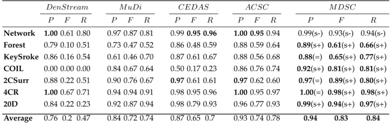
The comparative results are presented in Table 2. We first evaluate MDSC on four real data benchmarks. MDSC, on average,performs better than each peer algorithm despite requiring no parameter tuning for each specific stream.
Parameters for the peer algorithms are tuned (using the first n points in the stream as a training set) on each specific stream. On each stream we use a value of 4 forβ, so micro-clusters which have not been updated in 4λintervals are removed. We use λ = 100. Overall, purity levels are comparative with ACSC but each of four peer-algorithms are outperformed on the F1 and Rand Index metrics.
As these are real datasets, it is difficult to tell whether MDSC outperforms the peer algorithms because of the clustering mechanism itself or because the streams contain different densities. From the adaptivevalues, we can infer thatN etworkandF orestcontain a single level of density (Forest ≈ 0.2 and Network ≈ 0.11). However, on COIL andKeystroke, MDSC finds clusters with varying densities (0.005 to 0.26 on COIL, 0.002 to 0.01 on keyStroke). The progression of these streams using the three metrics is presented in Fig. 2 forCOILand Fig. 3 forKeyStroke.
To evaluate on streams that certainly contain different densities, we use two synthetic streams:2CSurrand20D. The comparative results are displayed in Table 2. MDSC outperforms the others on each of the three metrics.2CSurr consists of two clusters (one stationary and one dynamic) with different densities. The dynamic cluster is much more
TABLE 2: Average performance on each stream measured using Purity (P), F-Measure (F), Rand Index (R)
DenStream M uDi CEDAS ACSC M DSC
P F R P F R P F R P F R P F R Network 1.000.61 0.80 0.97 0.87 0.81 0.990.95 0.96 1.00 0.950.94 0.99(s-) 0.93(s-) 0.94(s-) Forest 0.79 0.10 0.51 0.73 0.47 0.52 0.86 0.48 0.59 0.88 0.59 0.64 0.89(s+) 0.61(s+) 0.66(s+) KeySroke 0.86 0.16 0.54 0.61 0.46 0.70 0.87 0.61 0.67 0.88 0.56 0.68 0.88(=) 0.65(s+) 0.77(s+) COIL 0.00 0.00 0.00 0.84 0.67 0.64 0.50 0.17 0.23 0.86 0.76 0.74 0.92(s+) 0.81(s+) 0.81(s+) 2CSurr 0.88 0.22 0.51 0.90 0.76 0.67 0.970.61 0.61 0.970.62 0.60 0.97(=) 0.89(s+) 0.80(s+) 4CR 1.000.67 0.71 0.94 0.94 0.91 0.98 0.95 0.96 1.000.95 0.97 1.00(=) 0.98(s+) 0.98(s+) 20D 0.84 0.22 0.23 0.92 0.87 0.94 0.98 0.79 0.93 0.96 0.77 0.93 0.99(s+) 0.94(s+) 0.97(s+) Average 0.76 0.2 0.47 0.84 0.72 0.74 0.87 0.65 0.7 0.93 0.74 0.78 0.94 0.83 0.84 0 2 4 6 8 10 12 14 0.5 1 Time
Pe
rformance
COIL Purity F1 Rand Index 1Fig. 2: Stream progression on the COIL stream.
0 2 4 6 8 10 12 14 16 0.5 Time
Pe
rformance
KeyStroke Purity F1 Rand Index 1Fig. 3: Stream progression on the Key Stroke stream.
compact and this is reflected in its-value of 0.012, much smaller than the other cluster with a density of0.029. We present a comparative performance with ACSC on this stream in Fig. 4. For illustrative purposes, we use a metric called ‘score’, which is simply the average of Purity, F1 and Rand Index, to show the progression. For these compar-isons, we use value of 0.02in ACSC. We use the second synthetic stream20Dto illustrate the problems with tuning a sensitive parameter such as this in a dynamic stream. 20D contains between 2 and 10 non-stationary clusters in 20 dimensions. The stream exhibits concept evolution, con-cept drift (both real and virtual) and clusters with varying densities, which was created using the previously described SynStream. We take a “training” set from the stream, which is the firstnsamples, and use the remaining stream as the “test”. The result is displayed in Table 3. If we take the first 1,000 points as a “test set”, the best value for is 0.03; if we take a test set of 5,000 points, the best value is much
0 5 10 15 20 25 30 35 40 45 50 0 0.2 0.4 0.6 0.8 1 Time
Score
Comparative Performance MDSC ACSC 1Fig. 4: Comparative performance on the 2CSurr stream. TABLE 3: Tuningparameter
1K 5K Full 0.1 0.62 0.72 0.73 0.09 0.62 0.72 0.74 0.08 0.60 0.75 0.77 0.07 0.62 0.76 0.74 0.06 0.63 0.74 0.73 0.05 0.63 0.74 0.74 0.04 0.65 0.68 0.72 0.03 0.67 0.62 0.70 0.02 0.66 0.55 0.69 0.01 0.47 0.50 0.64
larger at 0.07. Neither value gives the best performance over the entire stream: in this case the value that gives the best performance would be 0.08. This has implications in both the practicality of parameter tuning and also, which final result should be reported as a measure of the algorithm’s performance.
5.2 Tracking Clusters
To illustrate how discovered, online clusters can be tracked and their drift observed, we use two 2D data-streams for illustrative purposes: 2CSurr and 4CR. 2CSurr, as previously described, contains two clusters with varying densities and displays virtual concept drift. 4CR consists of 4 rotating clusters. The clusters rotate into positions pre-viously occupied by a different cluster, showing real drift. To illustrate this drift, we record the centre of discovered clus-ters at each time-step and display these centres in a scatter
IEEE TRANSACTIONS ON BIG DATA, VOL. XX, NO. XX, MONTH 2019
2CSurr Drift
9Fig. 5: Drift in 2CSurr stream. Blue cluster is stationary and red cluster drifting in direction of arrow. Center of clusters are recorded every time-step and the drift is captured and tracked. X Y 4CR Drift C 1 C 2 C 3 C 4
Fig. 6: Drift in 4CR, where the first 50,000 samples are presented. Underlying change represents a shift inP(y|X), the conditional probability of cluster y given position X. This underlying shift is tracked and can be seen in the overlap between each cluster’s trail.
plot. In the2CSurrstream, both clusters were tracked and their trails are displayed in Fig. 5. In 4CR, the clusters share a similar level of density, with={0.02,0.021,0.022,0.025}. We display the positions of each over the first 50,000 points in the stream. Clusters rotate into positions previously occupied by a different cluster so the underlying change represents a shift in P(y|x), the conditional probability of clustery given positionx. This underlying shift is tracked and can be seen in overlap between each cluster’s trail in Fig. 6.
5.3 Qualitative Evaluation
The previous data-steams are all labelled and we were able to objectively measure the performance of the algorithms according to the known ground-truth. In this section, we
quantitatively evaluate the algorithm on a real-world data stream in order to assess the utility of the discovered clus-ters. We use the internal metric Silhouette Coefficient to measure if the clusters are cohesive and well separated and we attempt to discover insights from these clusters and their behaviour over time. We evaluate the sensor readings from an Air-Quality monitoring site in the city of Leicester in the UK. We use this data to study the performance of MDSC only and not as a case-study in air-quality in Leicester since such a study would require data from a wider range of sites and would need to factor external influences, such as weather and wind etc.
The sensor records hourly measures of seven aspects of air quality. We take readings from January 2014 to April 2017
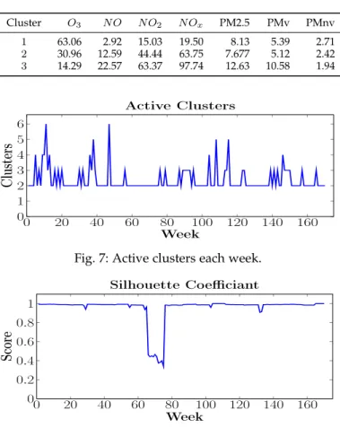
TABLE 4: Initial clusters in Week 1
Cluster O3 N O N O2 N Ox PM2.5 PMv PMnv 1 63.06 2.92 15.03 19.50 8.13 5.39 2.71 2 30.96 12.59 44.44 63.75 7.677 5.12 2.42 3 14.29 22.57 63.37 97.74 12.63 10.58 1.94 0 20 40 60 80 100 120 140 160 0 1 2 3 4 5 6 Week
Clusters
Active Clusters 1Fig. 7: Active clusters each week.
0 20 40 60 80 100 120 140 160 0 0.2 0.4 0.6 0.8 1 Week
Score
Silhouette Coeciant 1Fig. 8: Silhouette coefficient on the Air Quality stream. and read each point in the time order to simulate the original stream. To evaluate the stream on a weekly level, we setλ to 168 (24 hours by 7 days) andβ to 4. So, micro-clusters age every week and a micro-cluster which has not been updated for 4 weeks (roughly 1 month) is considered no longer relevant and removed. At each time-step, we record the mean, min and max values of each live cluster (i.e., the mean, min and max of the cluster’s constituent micro-clusters) and we record this for evaluation.
We examine the stream at a weekly level using appropri-ate values forλandβ, we could set these to different values for a monthly granularity (say,λ= 720, i.e., 24 hours times 30 days), daily (λ= 24), or real-time (λ= 1).
In week one, three clusters were discovered and their mean values are displayed in Table 4. Cluster 1 has high levels of Ozone (O3) but comparatively low levels of Ni-trates (N Ox) and Particulate Matter (P M2.5). Cluster 3 has a quarter of the levels ofO3but higher levels ofN Oxand P M2.5. Cluster 2’s levels lie between clusters 1 and 3. This suggest an inverse relationship between O3 andN Ox and P M2.5. Over the course of the stream (171 weeks), between 2 and 6 clusters are active each week. We use ‘active’ to mean that at least one new instance during the week was added to a live cluster. Clusters can still be live but inactive (no added points). The number of active clusters are displayed in Fig. 7 and the corresponding Silhouette Coefficient (SC) values are presented in Fig. 8.
The high SC scores suggest the live clusters are well separated and cohesive except for a ’wobble’ at approx-imately week 60. Of the active clusters, clusters 1 and 3
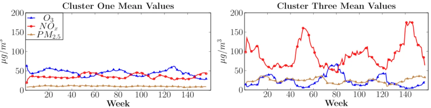
20 40 60 80 100 120 140 0 50 100 150 200 Week µg /m 3
Cluster One Mean Values O3 N Ox P M2.5 1 20 40 60 80 100 120 140 0 50 100 150 200 Week µg /m 3
Cluster Three Mean Values
1
Fig. 9: Mean values of persistent two clusters in Air Quality stream.
0 5 10 15 20 0 250 500 750 1,000 1,250 Time of Day Num ber in cluster
Total points clustered (weekly data)
Cluster 3 Cluster 1
1
Fig. 10: Relative sizes of cluster 1 and 3 and the hours they are most active.
are active throughout and represent the main underlying pattern. Their levels ofO3,N OxandP M2.5 are presented in Fig. 9. N Ox includes N O and N O2, andP M2.5 is the combined total of volatile and non-volatile P M2.5. So we reduce the seven measured variables to three just for clarity of display.
Looking at the progression of cluster 1, we can observe seasonal changes in the measured atmospheric gases. Levels ofO3 are higher in summer than in winter, the inverse of N Ox. These seasonal changes are tracked. Cluster 3 shows an exaggerated version of the same trend, much higher levels of N Ox and P M2.5 but lower levels of O3. It has been observed [19] that in an abundance of N Ox, O3 is ‘scavenged’ as it reacts withN Oxso this could explain the symmetry of the two levels in Cluster 3. The trends also suggest a correlation between N Ox and P M2.5. Both are comparatively low in cluster 1 and higher in cluster 3.
Clusters 1 and 3 capture the main underlying pattern of the stream. Cluster 1 represents a pattern of low levels of air pollution and is the largest cluster throughout. The relative sizes of each are presented in Fig. 10 along with the time-of-day they represent. The x-axis displays the 24 hours in a day and the y-axis represents the total number of potential hourly instances in the stream, in this case 1,197 (171 weeks ×7 days, 1,197 instances of 10am, for example). Cluster 1 can be seen to be much larger. For Cluster 3, its higher levels ofN Ox and P M2.5 occur more frequently at around 8am
and 6pm, typically rush-hour in a city. From this, we can infer that cluster 1 represents the ’usual’ levels of air quality, cluster 3 represents the rush-hour pattern and the remaining number of instances are distributed in clusters that represent anomalies or change. For example, cluster 5 was discovered in week 7 and represented a pattern of high particulate matter (≈26). This cluster was present until week 126 when it disappeared and was not replaced suggesting a change in the stream.
6
S
CALABILTY ANDR
OBUSTNESS TON
OISE6.1 Scalability
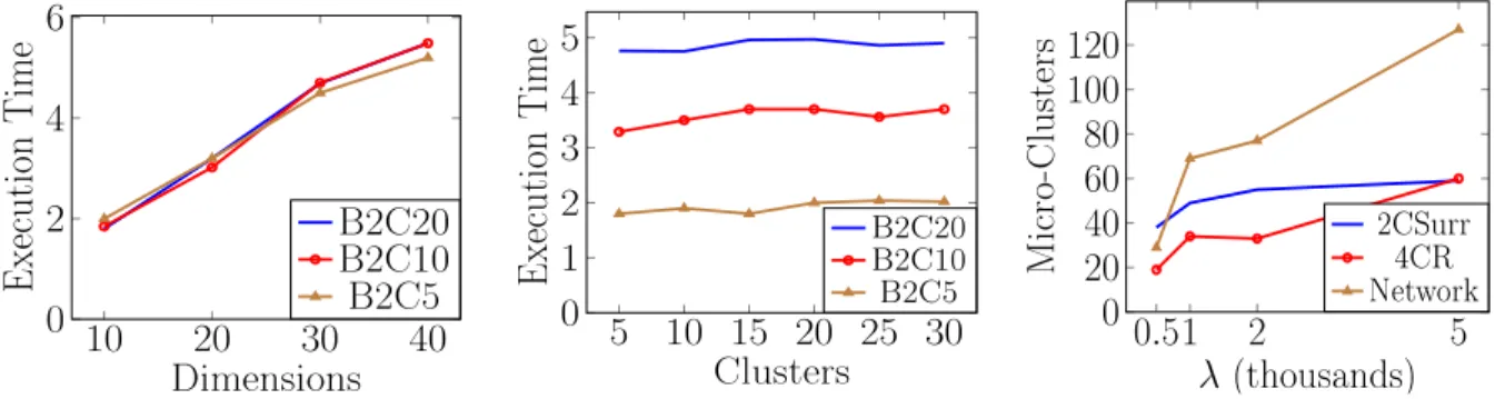
To evaluate the algorithm’s scalability, we generated syn-thetic data sets with varying dimensionality and number of clusters. As in [6], [13], the instances in each synthetic stream are drawn from a series of Gaussian distributions (each representing a cluster). The mean and variance of each distribution are shifted every 5,000 points during the generation process. We follow the notation used in [6] and [13] to describe the streams: ‘B’ indicates the number of data points (in hundreds of thousands), ‘C’ and ‘D’ indicate the number of clusters present and the dimensionality of each point, respectively. For example, B2C10D20 indicates the data set contains 200,000 data points of 20 dimensions, belonging to 10 different clusters.
The performance of the algorithm is measured in the execution time using aλ value of 10,000 and β = 5. The scalability of the algorithm, in terms of time, is evaluated against an increasing number of clusters and also increasing number of dimensions. In Fig. 11 (left), it can be seen that as the dimensionality increases, the execution time increases linearly, irrespective of the number of clusters, suggesting that the dimensionality is a more important factor than the number of clusters. This is confirmed when we fix the dimensionality and increase the number of natural clusters from 5 to 30, see Fig. 11 (centre). The stream takes roughly the same processing time as the number of cluster increases, with higher dimensional streams taking longer than lower dimensional ones. As the amount of clusters increases, the execution time increases only marginally.
As in [13] and [6], we evaluate the space complexity of MDSC in terms of micro-clusters present at different λ intervals. We use three previously described data streams to evaluate this; 2CSurr, 4CR and the Network Intrusion dataset. Fig. 11 (right) shows that asλincreases from 1,000 to 5,000, the number of micro-clusters generated increases,
10
20
30
40
0
2
4
6
Dimensions
Execution
Time
B2C20
B2C10
B2C5
15
10 15 20 25 30
0
1
2
3
4
5
Clusters
Execution
Time
B2C20 B2C10 B2C5 10
.
51
2
5
0
20
40
60
80
100
120
λ
(thousands)
Micro-Clusters
2CSurr4CR Network 1 Fig. 11: Scaling to the number of clusters, dimensions and memory requirements. TABLE 5: Noise sensitivity on the Network streamNoise Purity F-Measure R. Index Average#Nests
0% 0.99 0.91 0.88 2.14
3% 0.99 0.91 0.88 2.16
5% 0.99 0.91 0.87 2.2
8% 0.99 0.91 0.88 2.11
10% 0.99 0.91 0.88 2.05
TABLE 6: Noise sensitivity on 4CR
Noise Purity F-Measure R. Index Average#Nests
0% 0.99 0.94 0.96 4.12
3% 0.99 0.94 0.96 4.08
5% 0.99 0.94 0.95 4.09
8% 0.99 0.94 0.95 4.07
10% 0.99 0.93 0.95 4.04
at most, linearly on the Network Intrusion Dataset. On the
4CRand2CSurrstreams, the change is comparatively small asλincreases.
6.2 Noise
To evaluate how robust the algorithm is to noise, we intro-duce random samples to two datasets; Network Intrusion (first 100,000 samples) and 4CR. To introduce 1% noise, we replace 1% of the original data (inddimensions) with arti-ficial samples composed ofd-dimensional random numbers (within the same range of the original data), to evaluate with 5% noise, we replace 5% of the original data and evaluate with a λvalue of 1,000 and aβ of 5. We evaluate streams with varying levels of noise across the three external metrics and also report the average number of live clusters in the stream. The results on the two datasets are displayed in Tables 5 and 6, respectively.
It can be seen that the added noise has hardly any effect on the accuracy of the algorithm. Noise points are passed to the buffer, where they remain while they age and disappear, never joining the live clusters.
7
S
ENSITIVITYA
NALYSISTo examine the sensitivity of the algorithm to its parameters we evaluate across four streams: Forest,Network Intrusion,
2CSurrand4CR. We select these streams to cover a real data streams (Network, Forest), real concept drift (4CR) and multi-density clusters (2CSurr). MDSC requires two user-defined
parametersλandβ:λdetermines the rate at which micro-clusters age and the frequency at the which the buffer is examined (e.g. if λ = 1 the buffer is checked after every incoming point) whileβdetermines the age at which micro-clusters become irrelevant. These parameters determine the granularity at which the stream is analysed and should be judged according to the velocity of the stream, e.g., a stream with one point a second versus a stream with 1,000 points a second.
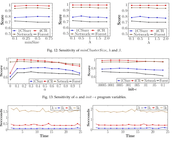
The sensitivity of these parameters to cluster quality is presented in Fig. 12. It can be seen that over a range of values thequantativeperformance is unaffected. Thequalitative values of the clusters will change though. For example, at a higherλ, long-term patterns will be discovered but smaller changes will be missed. Conversely, a smaller λ is more sensitive to change but will miss broader patterns. Along with these two user-defined parameters, there are three program values.minClusterSizedetermines the minimum size a cluster discovered in the buffer must be in order to be added to the live clusters. This is proportionate to the size of λ. For a smaller λ, the buffer is checked more frequently so smaller clusters should be allowed. When the buffer is checked infrequently, there will be potentially more instances in the buffer, so clusters are required to be larger. Fig. 12 (left) shows this parameter to be robust to values above 0 across each data stream tested. For all experiments, we use a value of 1% ofλwith a minimum value of 2.
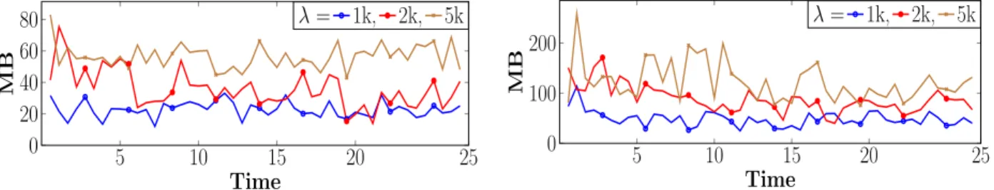
The parameter init- determines the initial value for when forming nests in the buffer and is used as the initial ‘starting point’ for the adaptive for each cluster. From Fig. 13 (right), it can be seen that, for values less than 0.01, the performance is stable across each stream. For all experiments in this work, we use a value of 0.001. The final program parameter is theαthreshold value, which defines a border nest in a cluster. This parameter is relative to the number of points clustered in the seed nest of a cluster. A larger seed will have a higher value for α. From Fig. 13 (left), we can see that the performance is stable across all streams with a value greater than 0 and less than 0.7. For all experiments discussed, we use a value of 0.1.
8
T
IME ANDM
EMORYR
EQUIREMENTSMDSC was shown to be scalable in terms of space and time in the previous section (Sec. 7). Here, we discuss the algorithm’s complexity and report empirical results on two real data-streams; Network Intrusion and Forest Cover. We
0.1 0.25 0.5 0.75 0.5 0.6 0.7 0.8 0.9 1 minSize
Score
1CSurr 4CR Network Forest 1 0.1 0.5 1 1.5 2.0 0.5 0.6 0.7 0.8 0.9 1 λScore
1CSurr 4CR Network Forest 1 0.1 0.5 1 1.5 2.0 0.5 0.6 0.7 0.8 0.9 1 λScore
1CSurr 4CR Network Forest 1Fig. 12: Sensitivity ofminClusterSize,λandβ.
0
0
.
1 0
.
2 0
.
3 0
.
4 0
.
5 0
.
6 0
.
7 0
.
8 0
.
9
1
0
.
6
0
.
8
1
α
Score1CSurr
4CR
Network
Forest
1
.00005 .0001 .0005 .001 .005
.01
.05
0.1
0.6
0.8
1
init-
Score1CSurr
4CR
Network
Forest
1
Fig. 13: Sensitivity ofαandinit−program variables.
5
10
15
20
25
0
0
.
5
1
1
.
5
Time
Seccondsλ
=
1k,
2k,
5k
15
10
15
20
25
0
1
2
Time
Seccondsλ
=
1k,
2k,
5k
1Fig. 14: Time requirements on Network Intrusion (left) and Forest-Cover (right) using differentλvalues.
refer to the number of clustered micro-clusters as N and the number in the outlier buffer asM. Typically,M is much smaller thanN.
The time complexity of the algorithm depends on the value ofλ as this determines how frequently we examine the buffer for new clusters. The complexity of joining a live cluster is O(N); a newly arriving point tests if it is density reachable with every micro-cluster in the discov-ered clusters. Periodically, when we examine the buffer, the processing time will increase. This increase is a function of change and noise. If there is no change or noise, then the buffer is empty and no further processing is required. If, however, the buffer is not empty, then the processing time increases to, in the worst case, O(M2) (The nest-building stage of the buffer check requiresO(M2)
and the clustering phase requires O(logM)). The time complexity of MDSC is O(N) and at every λintervals it requires an additional O(M2). In total, the algorithm requiresO(N+M2
λ ). Space is measured in terms of the number of micro-clusters that have been clustered plus the number in the outlier buffer:O(N+M).
We empirically measure the algorithm’s performance using differentλvalues. Large values mean micro-clusters will age more slowly, the buffer checked less regularly and therefore a greater a number of micro-clusters. We report
the time requirement in seconds (Fig. 14) and the memory requirements in MB (Fig. 15). We use a commercial profiler [21] to measure the memory requirements as the stream progresses. For clarity of display, we take the first 250,000 points in each stream.
For λ = 1,000 we plot the average of 10 windows (25 points), for a value of 2,000 we plot the average of 5 windows (25 points) and for λ = 5,000 we average 2 windows.
On the Network Intrusion Stream, the algorithm can process 1,000 points in, on average, 0.11 seconds, requiring, on average, 22MB. This rises with large values ofλ. Similar results are seen on the Forest Cover stream. It requires 0.14 seconds to process 1,000 points requiring 41MB, on average. MDSC’s time and memory requirements are compared with the four peer algorithms on the Network-Intrusion stream and the Forest-Cover stream. The streams are evalu-ated in windows of 1,000 and the average of each window (and the deviation) is reported in Table 7. ACSC requires the least time and memory with MDSC second showing comparable performance in second.
9
D
ISCUSSIONMDSC extends some of the swarm intelligence inspired aspects of density clustering introduced in ACSC, e.g.,
5
10
15
20
25
0
20
40
60
80
Time
MBλ
=
1k,
2k,
5k
15
10
15
20
25
0
100
200
Time
MBλ
=
1k,
2k,
5k
1Fig. 15: Memory requirements on Network Intrusion (left) and Forest-Cover (right) using differentλvalues. TABLE 7: Comparative time (secs.) and memory (MB)
re-quirements. Windows of size 1,000
Network Forest
Time (σ) Memory (σ) Time (σ) Memory (σ)
MDSC 0.11 (0.02) 22.0 (0.30) 0.14 (0.02) 31.1 (0.10)
ACSC 0.04(0.02) 21.5(0.07) 0.08(0.02) 21.5(0.09)
CEDAS 0.13 (0.03) 22.8 (0.10) 0.15 (0.02) 49.2 (0.30)
MuDi 0.19 (0.03) 27.1 (0.09) 0.49 (0.02) 56.4 (0.10)
DenStream 0.19 (0.07) 26.4 (0.11) 0.56 (0.09) 58.8 (0.30)
pheromone trails and the idea of micro-clusters forming ‘nests’. MDSC improves ACSC in two ways: clusters are online and the parameter is adaptive and local to each cluster. The adaptive has two benefits: 1) it removes the need to tune a sensitive, data-dependent parameter, and 2) it allows the discovery of multi-density clusters. This can be seen in the comparative performance; on the streams which contain multi-densities (COIL,Key Stroke,2CSurrand20D), the proposed algorithm finds a better clustering solution. When the stream contains a single density (Network,Forest,
4CR), the performance is comparable. The reason for this is the adaptiveand the way it is identified. Clusters are dis-covered in order of density, i.e., more compact clusters are identified first. This allows the discovery of clusters (with a smaller ) embedded in larger sparser clusters (with a higher). Discovered clusters are uniquely labelled (cluster 1, cluster 2, . . . ) and can therefore be tracked over time. This was shown in the 2D synthetic data sets; the underlying drift in the stream was discovered and tracked. This was further illustrated in the case study on the Leicester air-quality dataset. Discovered clusters were tracked despite seasonal changes in the monitored atmospheric gases. Underlying patterns were discovered along with their deviations, and cyclic patterns were revealed. These live, labelled clusters allow us to infer a broader picture of what is happening in the stream and we can do this at different granularities.
We examined the stream at a weekly granularity. The granularity is controlled by two parameters:λ, which deter-mines the rate at which data ages, andβ, which determines how long data is relevant. Changing these two parameters dictate the granularity at which the stream is analysed. Analysing a stream at different granularities in parallel could catch brief anomalies while revealing the broader behaviour of the stream.
Along with λ and β, MDSC uses three program
vari-ables. These were shown to be stable on different data and not sensitive to small changes. These static, global values facilitate adaptive, local parameters for each cluster. minP ointsdetermines the minimum size a cluster must be. This value is proportional toλ. Clusters each have a local value for and this is discovered usinginit- as a starting point. Similarly, each cluster has a local value threshold which determines the border micro-clusters in that cluster. A program-valueαis a constant in the formulation of this parameter threshold. The same value for each of these program variables are used on each data stream evaluated in the experimental section;minP oints=max(λ∗.01,2),
init-= 0.001, andα= 0.1. The use of these program-values to discover adaptive local values removes the need to tune sensitive user-defined parameters in a stream.
Sensitive user-defined parameters in a non-stationary data stream are potentially problematic and not much con-sideration is given to their practicality. Often, parameters are reported but not the method used to tune these parameters. Following traditional machine learning methods, we could take a subset of the stream and use this test-set to tune the parameters. However, in a dynamic environment, sensitive parameters are likely to change over time, especially (as is realistic) if the stream contains concept evolution and multi-density clusters. Furthermore, it may be easy to tune these parameters on a test stream when the ground truth is known, but in practical terms this is unrealistic. If a stream clustering algorithm requires sensitive user parameters, methods to tune these parameters should be outlined and ideally, these methods should facilitate periodic parameter updates.
10
C
ONCLUSIONSIn this paper, we proposed a Multi Density Stream Clus-tering (MDSC) algorithm for on-line clusClus-tering of dynamic data streams. MDSC attempts to address two problems -the multi-density problem in density clustering whereby clusters can only be discovered using a single concept of density () and the problem of discovering and tracking
change in a dynamic stream. The algorithm addresses the former by discovering clusters with an adaptive local to each cluster. To address the second problem of tracking change, we maintain discovered clusters online. We label each and observe its behaviour over time. Live clusters are composed of smaller micro-clusters which are subject to an ageing function. A newly arriving point is, if appropriate, assigned to an existing cluster; otherwise, it is assigned to an existing outlier micro-cluster, or joins the buffer as a
new micro-cluster. New clusters are periodically discovered among the outliers. Micro-clusters which have not absorbed new data age and are deleted if they are considered no longer relevant. This allows clusters to adapt to the under-lying drift and because of their unique label we can track the pattern of this drift.
MDSC was evaluated across a number of benchmark streams exhibiting concept evolution, real and virtual con-cept drift, and multi-density clusters It was shown to perform favourably to four peer algorithms. It was also qualitatively evaluated on a real-life air-quality monitoring stream. Results show that it can identify and track underly-ing patterns despite seasonal changes and cyclic behaviour. MDSC could discover and track patterns such as rush-hour and a cyclic increase in pollutants during winter. A correlative relationship between certain pollutants and an inverse relationship between others were observed. MDSC requires two user-defined parameters which depend on the velocity of the stream and the granularity at which the user wishes to analyse the stream. Along with these two user-defined parameters, three program-variables which do not require any manual tuning are used. These static, global values facilitate adaptive, local parameters for each cluster.
Experimental results suggest that MDSC is a scalable, on-line clustering algorithm and is robust to change and noise. It can discover qualitatively useful patterns underlying the data at different levels of granularity.
Future directions and extensions to MDSC could include exploring the potential of using the clusters as an ensemble of one-class classifiers for dynamic classification. Similarly, the clusters could potentially be used to train a set of regression models that make short term predictions for the discovered patterns.
R
EFERENCES[1] C. C. Aggarwal, J. Han, J. Wang, and P. S. Yu, “A framework for clustering evolving data streams,” Proc. 29th Int. Conf. Very Large Data Bases, vol. 29, pp. 81–92, 2003.
[2] E. Amiga, J. Gonzalo, J. Artiles, J. and F. Vedejo, “A comparison of extrinsic clustering evaluation metrics based on formal con-straints,” Information Retrieval, vol. 12, no. 4, pp. 461–486, 2009. [3] A. Amini, H. Saboohi, T. Herawan, and T.Y Wah. “MuDi-Stream:
A multi density clustering algorithm for evolving data stream,” Journal of Network and Computer Applications, vol. 59, pp. 370– 385, 2016.
[4] A. Amini, T.Y. Wah and H. Saboohi. “On density-based data streams clustering algorithms: A survey,” Journal of Computer Science and Technology, vol. 29, no. 1, pp. 116–141, 2014. [5] A. Bifet, G. Holmes, R. Kirby, and B. Pfahringer, “MOA: Massive
online analysis,” Journal of Machine Learning Research, vol. 11, pp. 1601–1604, 2010.
[6] F. Cao, M. Ester, W. Qian, and A. Zhou, “Density-based clustering over an evolving data stream with noise,” SDM, vol. 6, pp. 328– 339, 2006.
[7] C. Carmelo, A. Ferro, R. Giugno, G. Pigola, and A. Pulvirenti. “Enhancing density-based clustering: Parameter reduction and outlier detection,” Information Systems, vol. 38, no. 3, pp. 317– 330, 2013.
[8] M. T. Chao, “Data stream classification guided by clustering on nonstationary environments and extreme verification latency,” Proc. 2015 SIAM Int. Conf. Data Mining, pp. 873–881, 2015. [9] M. Dorigo, M. Birattari, and T. Stizle,“Ant colony optimization,”
IEEE Comput. Intell. Mag., vol. 1, no. 4, pp. 28–39, 2006.
[10] S. Ding, J. Zhang, H. Jia, and J. Qian. “An adaptive density data stream clustering algorithm.” Cognitive Computation, vol. 8, no. 1, pp. 30–38, 2016.
[11] M. Ester, H. P. Kriegel, J. Sander, and X. Xu,“A density-based algorithm for discovering clusters in large spatial databases with noise,” KDD, vol. 96, pp. 226–231, 1996.
[12] G. Esfandani and H. Abolhassani. ”MSDBSCAN: multi-density scale-independent clustering algorithm based on DBSCAN,” Proc. Int. Conf. on Advanced Data Mining and Applications, 2010. [13] C. Fahy, S. Yang, and M. Gongora. “Ant colony stream clustering:
A fast density clustering algorithm for dynamic data streams,” IEEE Trans on Cybern, vol. 49, no. 6, pp. 2215–2228, June 2019. [14] C. Fahy, S. Yang, and M. Gongora. “Finding multi-density clusters
in non-stationary data streams using an ant colony with adaptive parameters.” In Proc. 2017 IEEE Congress on Evolutionary Com-putation, pp. 673–680, 2017.
[15] A. Forestiero, C. Pizzuti, and G. Spezzano, “A single pass al-gorithm for clustering evolving data streams based on swarm intelligence,” Data Mining and Knowledge Discovery, vol. 26, no. 1, pp. 1–26, Nov. 2011.
[16] B. J. Frey and D. Dueck, “Clustering by passing messages between data points,” Science 315.5814, pp. 972-976, 2007.
[17] J. A. Hartigan and M. A. Wong, “Algorithm AS 136: A k-means clustering algorithm,” Applied Statistics, vol. 28, no. 1, pp. 100– 108, 1979.
[18] R. Hyde, P. Angelov, and A. R. MacKenzie, “Fully online clus-tering of evolving data streams into arbitrarily shaped clusters,” Information Sciences, vol. 382-383, pp. 96–114, 2017.
[19] W. B. Innes, “Effect of nitrogen oxide emissions on ozone levels in metropolitan regions,” Environmental Science and Technology, vol. 15, no. 8, pp. 904–912, 1981.
[20] C. Isaksson, M.H Dunham, and M. Hahsler. “SOStream: Self or-ganizing density-based clustering over data stream??. In Interna-tional Workshop on Machine Learning and Data Mining in Pattern Recognition (pp. 264-278). Springer, Berlin, Heidelberg. July 2012. [21] J-Profiler: Java Profiler. https://www.ej-technologies.com/
products/jprofiler/overview.html, 21 11 2017.
[22] N. Jardine and C. J. van Rijsbergen, “The use of hierarchic cluster-ing in information retrieval,” Information Storage and Retrieval, vol. 7, no. 5, pp. 217–240, Dec. 1971.
[23] D. Karaboga, and B. Basturk.“ A powerful and efficient algorithm for numerical function optimization: artificial bee colony (ABC) algorithm”. Journal of Global Optimization, vol. 39, no. 3, pp. 459– 471, 2007
[24] P. Kranen, I. Assent, C. Baldauf, and T. Seidl, “The ClusTree: indexing micro-clusters for anytime stream mining.” Knowledge and Information Systems, vol. 29, no. 2, pp. 249–272, 2011. [25] J. Li, D. Maier, K. Tufte, V. Papadimos, and P. A. Tucker,
“Se-mantics and evaluation techniques for window aggregates in data streams,” In: Proc. 2005 ACM SIGMOD Int. Conf. on Management of Data, pp. 311–322, 2005.
[26] X. Li, Y. Ye, M. J. Li,and M. K. Ng, “On cluster tree for nested and multi-density data clustering,” Pattern Recognition, vol. 43, no. 9, pp. 3130–3143, 2010.
[27] B. Liu, “A Fast Density-Based Clustering Algorithm For Large Databases,” Proc. 5th Int. Conf. Machine Learning and Cybern., 2006.
[28] W. M. Rand, “Objective criteria for the evaluation of clustering methods,” J. of the American Statistical Assoc., vol. 66, no. 336, pp. 846, Dec. 1971.
[29] C. W. Reynolds, “Flocks, herds and schools: A distributed behav-ioral model,” ACM SIGGRAPH Computer Graphics, vol. 21, no. 4, pp. 25–34, Aug. 1987.
[30] P. J. Rousseeuw and L. Kaufman. “Finding Groups in Data,” Wiley Online Library, 1990.
[31] P. N. Suganthan,” Particle swarm optimiser with neighbourhood operator”. In: Proc. 1999 IEEE Congress on Evol. Comput., vol. 3, pp. 1958–1962, 1999.
[32] P.-N. Tan, M. Steinbach, and V. Kumar, Introduction to Data Mining. Boston, MA: Pearson/Addison-Wesley, 2005, ch. 9, pp. 147–160.
[33] D. M. Tax and R.P Duin, 2004. “Support vector data description,” Machine learning, vol. 54, no. 1, pp. 45-66. 2004.
[34] L. Tu and Y. Chen, “Stream data clustering based on grid density and attraction,” ACM Trans. Knowledge Discovery from Data, vol. 3, no. 3, pp. 1–27, Jul. 2009.
[35] L. Wan, W. K. Ng, X. H. Dang, P. S. Yu, and K. Zhang, “Density-based clustering of data streams at multiple resolutions,” ACM Trans. Knowledge Discovery from Data, vol. 3, no. 3, pp. 1–28, Jul. 2009.
[36] C. D. Wang, J. H. Lai, D. Huang, and W. S. Zheng, “SVStream: A support vector based algorithm for clustering data streams,” IEEE Trans on Knowledge and Data Engineering, 2011.
[37] F. Wilcoxon and R. A. Wilcox. “Some rapid approximate statistical procedures”. Lederle Laboratories, 1964.
[38] T. Zhang, R. Ramakrishnan, and M. Livny, “Birch: A new data clustering algorithm and its applications,” Data Mining and Knowledge Discovery, vol. 1, no. 2, pp. 141–182, 1997.
[39] Z. Xiong, R. Chen, Y. Zhang, and X. Zhang. “Multi-density dbscan algorithm based on density levels partitioning.” Journal of Infor-mation and Computational Science, vol. 9, no. 10, pp. 2739–2749, 2012.
[40] X. S. Yang, “Firefly algorithm, stochastic test functions and design optimisation,” arXiv preprint arXiv:1003.1409. 2010.
Conor Fahyreceived a B.Sc. degree in Com-puter Science from Dublin City University, Ire-land in 2004. He received an M.Sc. degree in Intelligent