Santa Clara University
Scholar Commons
Engineering Ph.D. Theses Student Scholarship
6-2017
Towards Efficient Resource Provisioning in
Hadoop
Peter P. Nghiem
Santa Clara University, [email protected]
Follow this and additional works at:http://scholarcommons.scu.edu/eng_phd_theses Part of theComputer Engineering Commons
This Thesis is brought to you for free and open access by the Student Scholarship at Scholar Commons. It has been accepted for inclusion in Engineering Ph.D. Theses by an authorized administrator of Scholar Commons. For more information, please [email protected].
Recommended Citation
Nghiem, Peter P., "Towards Efficient Resource Provisioning in Hadoop" (2017).Engineering Ph.D. Theses. 10. http://scholarcommons.scu.edu/eng_phd_theses/10
Department of Computer Engineering
June 2017
I HEREBY RECOMMEND THAT THE THESIS PREPARED UNDER MY SUPERVISION BY
Peter P. Nghiem
ENTITLED
Towards Efficient Resource Provisioning in Hadoop
BE ACCEPTED IN PARTIAL FULFILLMENT OF THE REQUIREMENTS FOR THE DEGREE OF
DOCTOR OF PHILOSOPHY IN COMPUTER SCIENCE AND ENGINEERING
] / "f
,7 L-^4.. "tl. Ut...^^ •<„. }{"'t»-''''s,,...^t.^_^
Chair of Doctoral Committee Member of Doctorai Committee
Member of DoctdFraI Committee Member of Doctoral Committee
W^iu£^5 &^
Santa Clara University
Department of Computer Engineering
June 2017
I HEREBY RECOMMEND THAT THE THESIS PREPARED UNDER MY SUPERVISION BY
Peter P. Nghiem
ENTITLED
Towards Efficient Resource Provisioning in Hadoop
BE ACCEPTED IN PARTIAL FULFILLMENT OF THE REQUIREMENTS FOR THE DEGREE OF
DOCTOR OF PHILOSOPHY IN COMPUTER SCIENCE AND ENGINEERING
_______________________ _______________________
Chair of Doctoral Committee Member of Doctoral Committee
_______________________ _______________________
Member of Doctoral Committee Member of Doctoral Committee
_______________________ _______________________
i
TOWARDS EFFICIENT RESOURCE PROVISIONING IN HADOOP
by
Peter P. Nghiem
THESIS
Submitted in partial fulfillment of the requirements for the degree of Doctor of Philosophy
in Computer Science and Engineering School of Engineering
Santa Clara University
Santa Clara, California June 2017
ii
Abstract
Considering recent exponential growth in the amount of information processed in Big Data, the high energy consumed by data processing engines in datacenters has become a major issue, underlining the need for efficient resource allocation for better energy-efficient computing. This thesis proposes the Best Trade-off Point (BToP) method which provides a general approach and techniques based on an algorithm with mathematical formulas to find the best trade-off point on an elbow curve of performance vs. resources for efficient resource provisioning in Hadoop MapReduce and Apache Spark. Our novel BToP method is expected to work for any applications and systems which rely on a trade-off curve with an elbow shape, non-inverted or inverted, for making good decisions. This breakthrough method for optimal resource provisioning was not available before in the scientific, computing, and economic communities.
To illustrate the effectiveness of the BToP method on the ubiquitous Hadoop MapReduce, our Terasort experiment shows that the number of task resources recommended by the BToP algorithm is always accurate and optimal when compared to the ones suggested by three popular rules of thumbs. We also test the BToP method on the emerging cluster computing framework Apache Spark running in YARN cluster mode. Despite the effectiveness of Spark’s robust and sophisticated built-in dynamic resource allocation mechanism, which is not available in MapReduce, the BToP method could still consistently outperform it according to our Spark-Bench Terasort test results. The performance efficiency gained from the BToP method not only leads to significant energy saving but also improves overall system throughput and prevents cluster underutilization in a multi-tenancy environment. In General, the BToP method is preferable for workloads with identical resource consumption signatures in production environment where job profiling for behavioral replication will lead to the most efficient resource provisioning.
iii
Keywords
Best Trade-off Point; Hadoop MapReduce; Apache Spark; YARN; Optimal resource provisioning; Dynamic resource allocation; Energy efficiency; Performance efficiency; Yield curve; Exponential decay curve; Elbow curve.
iv
Acknowledgments
First, I would like to thank my PhD advisor, Professor Dr. Silvia M. Figueira for accepting me to the PhD program under her supervision, supporting my research, guiding me throughout the academic process, having faith in my innovative ideas and hard work, and examining and proofreading my journal research papers.
I would like to thank all the members of my doctoral committee, who are Professor Dr. Nicholas Tran, Professor Dr. Yi Fang, Professor Dr. Weijia Shang, and Professor Dr. Ahmed Amer, for their continuing support, encouragement, suggestion, and advice in my research and studies for the PhD degree in Computer Science and Engineering. I particularly would like to express my appreciation to Professor Dr. Nicholas Tran who thoroughly examined my journal research paper and provided good feedback in every step of the way. I also particularly would like to express my appreciation to Professor Dr. Yi Fang for letting me use his entire group research disk space on SCU Design Center’s Hadoop cluster for my benchmark testing and examining my journal research paper. I would like to especially thank SCU Design Center System Administrator Chris Tracy for setting up, configuring, and maintaining any necessary Hadoop MapReduce, Spark, and Spark-Bench suite and benchmark tools, and allocating additional disk space sufficient for my research on SCU Design Center’s Hadoop cluster whenever needed. Special thanks go to Professor Dr. JoAnne Holliday, Professor Dr. Ahmed Amer, and Professor Dr. Weijia Shang for advising me in the Master of Science degree in Computer Science and Engineering. In addition, I would like to thank the late Professor Dr. Robert Parden for advising me in the Master of Science degree in Engineering Management and Leadership.
I would like to thank the Chair of SCU Computer Engineering department, Professor Dr. Nam Ling for his continuing support, guidance, and advice on the academic process and requirements of SCU graduate programs in Computer Science and Engineering. I also would like to thank the Dean of SCU School of engineering, Dean Professor Dr. Godfrey Mungal for his continuous support and advice, and the Dean’s Fellowship for my continuing PhD research at SCU. Finally, I would like to thank all the professors who have
v
giving me invaluable knowledge in their courses and advices over the decades of my graduate engineering studies at SCU.
Last, but not least, I would like to thank my parents, my sisters and brothers, my other relatives, and my friends, who have supported my graduate engineering studies and academic goal at SCU.
vi
Table of Contents
Abstract ………..ii
Keywords ………..iii
Acknowledgments ……….…...iv
Table of Contents ……….vi
List of Figures ……….viii
List of Tables ……….…xi
Chapter 1 Introduction ……….………...1
1.1 Acknowledgment of Funding and Use of Facilities ………..1
1.2 Thesis Overview ………...…….1
1.3 Thesis Contributions ………..2
Chapter 2 Best Trade-off Point Method (BToP) ……….………..6
Chapter 3 Efficient Resource Provisioning in MapReduce ………...13
3.1 Pertinent Research in Performance Efficiency of MapReduce ……….13
3.2 Background Knowledge on MapReduce ……...………14
3.2.1 Hadoop Distributed File System (HDFS) ………..…..……15
3.2.2 MapReduce Programming Model ………..………..16
3.2.3 MapReduce Job Execution on YARN ………...………..18
3.3 MapReduce Resource Provisioning ………..20
3.4 BToP Algorithm for Optimal Resource Provisioning ………23
3.5 Design, Analysis, and Implementation of BToP Algorithm ……….….25
3.5.1 Experimental Background ………25
3.5.2 Preview Data ………...………...…..29
3.5.3 Process for Ascertaining Optimal Number of Tasks ………30
3.6 Resource Provisioning with BToP Method vs. Popular Rules of Thumbs ….39 Chapter 4 Efficient Resource Provisioning in Spark ……….44
4.1 Background Knowledge on Apache Spark …………...……….46
vii
4.1.2 Distributed Execution in Spark ……….……….50
4.1.3 Spark’s Dynamic Resource Allocation (DRA) ………..51
4.2 Spark-Bench Terasort Experiment with BToP Method ……….55
4.3 Analysis of Spark with BToP method vs. Spark with DRA enabled ……....67
4.3.1 Performance Gain ……….67
4.3.2 Energy Saving ………...70
Chapter 5 Conclusion and Future Work ………....73
viii
List of Figures
Fig. 1 Flowchart of Best Trade-off Point Method ………...3
Fig. 2 Best Trade-off Point Algorithm for an Elbow Curve (Noninverted) ………….…7
Fig. 3 Best Trade-off Point Algorithm for an Inverted Elbow Curve ………9
Fig. 4 Architecture of Hadoop Distributed File System (HDFS) ………..15
Fig. 5 MapReduce Data Flow ………...17
Fig. 6 MapReduce Job Execution on YARN ………19
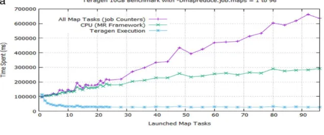
Fig. 7 Graphs of time spent by all map tasks, CPU, and Teragen execution versus number of launched map tasks. The runtime elbow curves of Teragen (a) 10 GB, (b) 100 GB and (c) 1 TB workloads plotted at different y-axis scales all appear to have the best trade-off points for performance efficiency at around 10 map tasks. But that is refuted by our algorithm as a visual misperception of different granularities at low magnification ..……….21
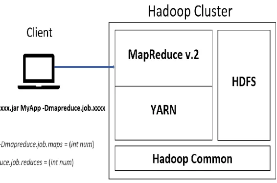
Fig. 8 Allocating Task Resources to Sample Executions on the Target Hadoop Cluster ………26
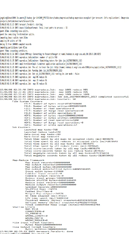
Fig. 9 Test Run of Terasort 100GB with –Dmapreduce.job.reduces = 32 ……..…...27
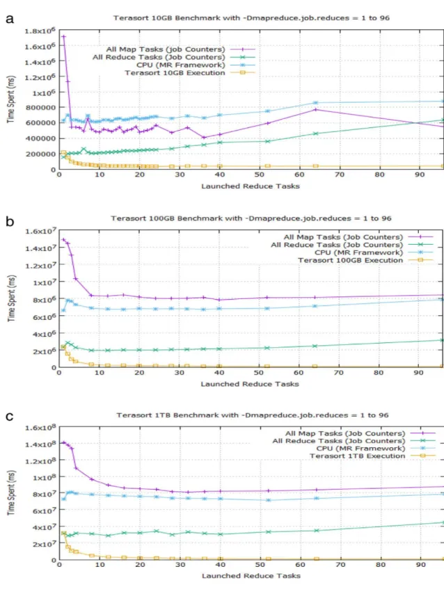
Fig. 10 Graphs of time spent by all map tasks, all reduce tasks, CPU, and Terasort execution versus number of launched reduce tasks. The runtime elbow curves of Terasort (a) 10 GB, (b) 100 GB and (c) 1 TB workloads plotted at different y-axis scales all appear to have the best trade-off points for performance efficiency at around 10 reduce tasks. But that is disproved by our algorithm as a visual misperception of different granularities at low magnification .………...28
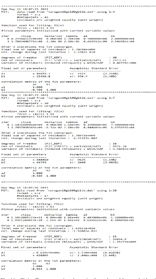
Fig. 11 Fitting Teragen preview data using Levenberg–Marquardt Algorithm (LMA), aka the damped least-squares (DLS) method ...………...31
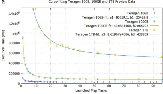
Fig. 12 Fitted runtime elbow curves of (a) Teragen and (b) Terasort 10 GB, 100 GB, and 1 TB workloads versus number of launched map/reduce tasks, and their fit parameters a and b in the graph function f ( x )= ( a / x ) + b ...………....33
Fig. 13 Applying BToP algorithm to Teragen 10 GB, 100 GB, and 1 TB workloads, our program tabulates the number of tasks over range of slopes, acceleration over range of slopes, and recommended acceleration, slope, and optimal
ix
number of tasks over range of incremental changes in acceleration per slope increment, to output the final recommended optimal numbers of
tasks for each Teragen workload ...……….………35
Fig. 14 The optimal number of tasks for Teragen 10 GB, 100 GB, and 1 TB workloads are identified by the major plateaus lasting at least eight increments on the graphs. The algorithm searches for break points in the changes in acceleration and outputs: (a) recommended acceleration, (b) corresponding slope and (c) task resources versus change in acceleration per slope increment ………..……..36
Fig. 15 Applying BToP algorithm to MR Terasort 10 GB, 100 GB, and 1 TB workloads, our program tabulates the number of tasks over range of slopes, acceleration over range of slopes, and recommended acceleration, slope, and optimal number of tasks over range of incremental changes in acceleration per slope increment, to output the final recommended optimal numbers of tasks for each Terasort workload ..……….37
Fig. 16 The optimal numbers of tasks for Terasort 10 GB, 100 GB, and 1 TB workloads are identified by the major plateaus lasting at least eight increments on the graphs. The algorithm searches for break points in the changes in acceleration and outputs: (a) recommended acceleration, (b) corresponding slope and (c) task resources versus change in acceleration per slope increment ………38
Fig. 17 Fitted elbow curves of Terasort 10 GB, 100 GB, and 1 TB workloads from sampled executions verify the accuracy of our algorithm for optimal resource provisioning in contrast to the unreliable number of reducers calculated from three popular rules of thumb (A, B, and C(2)), which could lead to significant waste of computing resources and energy ...………...39
Fig. 18 Apache Spark Echosystem ………...47
Fig. 19 Spark Architecture in Cluster Mode ………..48
Fig. 20 DAG visualization of a simple word count job …………..………50
Fig. 21 Apache Spark 1.5.0 Dynamic Resource Allocation Properties ………...52
Fig. 22 SparkBench env.sh settings for the experiment with 48 executors …………...57
Fig. 23 Plots of Preview data of duration vs. executors of SparkBench Terasort 10GB, 100GB and 1TB of data at different vertical scales ………...60
Fig. 24 Fitting Spark-Bench Terasort preview data points to the function f(x) = (a/x)+b ……….62
x
Fig. 25 Fitted runtime vs. executors’ elbow curves of SparkBench Terasort 10GB, 100GB, and 1TB of data, and their runtimes with Dynamic Resource
Allocation (DRA) enabled …..………...63 Fig. 26 Applying BToP algorithm to Spark-Bench Terasort 10 GB, 100 GB and
1 TB workloads to tabulate the number of executors over range of slopes, acceleration over range of slopes, and recommended acceleration, slope, and optimal number of executors over range of incremental changes in acceleration per slope increment, to output the final recommended
optimal numbers of executors for each workload …...………...…64 Fig. 27 The optimal numbers of executors for Spark-Bench Terasort 10 GB,
100 GB, and 1 TB workloads are identified by the major plateaus lasting at least seven increments on the graphs. The algorithm searches for break points in the changes in acceleration and outputs: (a) recommended acceleration, (b) corresponding slope and (c) executors versus change in acceleration per slope increment ………...………65
xi
List of Tables
Table 1 Performance of Spark-Bench Terasort with Dynamic Resource Allocation (DRA) enabled vs. Spark using BToP method (with DRA disabled) ……….68 Table 2 Energy savings in using Spark with BToP method in lieu of Dynamic
Resource Allocation (DRA) enabled for Spark-Bench Terasort of 10GB, 100GB, and 1TB ……….71
1
Chapter 1
Introduction
1.1 Acknowledgment of Funding and Use of Facilities
The work presented in this thesis was mostly supported by the author’s own federal student loans. The second part of the author’s research during the academic year 2016-2017 was supported in part by a fellowship from the Dean of SCU School of Engineering. The author gratefully acknowledges use of the Hadoop cluster of SCU School of Engineering Design Center.
1.2 Thesis Overview
This thesis addresses the problem of allocating the right amount of task resources for a workload in Hadoop MapReduce and similarly, the right number of executors for a workload in Apache Spark. It relates generally to resource provisioning in software framework and computing systems including but not limited to parallel and distributed processing of Big Data by large computer clusters. More specifically, it relates to methods for determining the number of task resources for each different workload to optimally balance performance and energy efficiency.
Gartner Inc. research firm has forecasted that the rapidly-growing cloud ecosystem will have up to 25 billion IoT sensor devices connected by 2020 [15]. This large number of IoT devices will generate hundreds of zettabytes of information in the cloud to be analyzed by Big Data processing engines, such as Hadoop MapReduce and Apache Spark, and other analytics platforms to deliver practical value in business, technology, and manufacturing processes for better innovation and more intelligent decisions. In such an era of exponential growth in Big Data, energy efficiency has become an important issue for the ubiquitous Hadoop and Spark ecosystems.
It is now established that the energy consumption cost of a server over its useful life has far exceeded its original capital expenditure [27]. Gartner estimated in a July 2016 report that Google at the time had 2.5 million servers and counting [13]. As such, the energy
2
consumption associated with datacenters has become a major concern as more companies have more datacenters with over a million servers. In fact, datacenter electricity consumption is projected to increase to roughly 140 billion kilowatt-hours annually by 2020, the equivalent annual output of 50 power plants, costing American businesses $13 billion annually in electricity bills and emitting nearly 100 million metric tons of carbon pollution per year [40]. A large portion of datacenter workloads is processed by Hadoop MapReduce and Apache Spark, popular de facto standard frameworks for Big Data processing, which have been adopted by many world’s leading cloud computing providers and top Big Data companies, among many other organizations and institutions. As such, we could reduce this datacenter energy expense which is largely incurred for Big Data processing, through more efficient resource provisioning in MapReduce and Spark among other data processing frameworks.
There is a growing amount of research work dedicated to making these Big Data processing frameworks more energy efficient. However, there has been no definite answer to the question of what optimal number of resources should be allocated for a job to get the most efficient performance from MapReduce until now when this proposed Best Trade-off Point method is made available. Hadoop developers and users previously had to rely on popular but inaccurate rules of thumb widely circulated in industry for their MapReduce job execution, leading to significant unintended waste of computing resources and energy. This thesis proposes an innovative method and algorithm for obtaining the best trade-off between performance and computing resources for energy efficiency in any workload running on Hadoop MapReduce and Apache Spark among other applications and systems which rely on a trade-off elbow curve, non-inverted or inverted, for good decision making.
1.3 Thesis Contributions
This thesis makes the following contributions:
We develop the Best Trade-off Point (BToP) method which is applicable to any system relying on a trade-off elbow curve for making good decisions (Fig. 1). It provides a general approach and techniques based on an algorithm with mathematical formulas to find the best trade-off point on an elbow curve, non-inverted as f(x)=(a/x)+b or inverted as f(x)=-(a/x)+b, of performance vs. resources.
3
We present the BToP method as a job profiling method for optimal resource provisioning for any MapReduce workload by getting runtime samples of the cluster targeted for calibration as reference points for curve-fitting and computation to find the best trade-off point on the runtime elbow curve (Fig. 1).
We then apply the BToP method to Apache Spark running in YARN cluster mode. We show how preview data can be extracted from sample executions of different workloads on Spark YARN cluster computing system targeted for calibration as reference points for curve-fitting and computation to find the best trade-off point on the runtime elbow curve (Fig. 1).
4
We also provide a step-by-step computation process with mathematical formulas for the runtime graph function f (x ) = ( a / x ) + b, its first derivative, its second derivative, the Chain Rule, and search conditions for breakpoints and major plateaus to find the optimal number of tasks.
We design an algorithm for best trade-off point to take the single parameter a in the graph function f (x ) = ( a / x )+ b for a workload as input and output the exact recommended optimal number of task resources.
We validate our design and techniques using experiments on a real 24-node homogeneous Hadoop cluster with Teragen and Terasort components of the Terasort benchmark test with 10 GB, 100 GB and 1 TB of data (Fig. 8 in Section 3.5.1).
We verify and compare the results of our algorithm against the numbers of tasks suggested by three currently well-known rules of thumbs widely circulated in industry using the fitted runtime elbow curves. We also provide a numerical example of potential energy savings from the results.
The results of our evaluation show that our approach consistently provides accurate and optimal number of task resources for any MapReduce workload to achieve performance efficiency while the numbers of reduce tasks suggested by the three popular rules of thumb are inaccurate leading to significant unintended waste of computing resources and energy as shown in Fig. 17 in Section 3.6.
We, then, further verify the Best Trade-off method with Apache Spark workloads by executing Spark-Bench Terasort with 10GB, 100GB, and 1TB of data on the same real 24-node homogeneous Hadoop cluster, albeit with a different and newer
CDH (Cloudera's Distribution Including Apache Hadoop) version. The Spark-Bench Terasort tests were measured with Spark’s built-in dynamic resource allocation feature first set to enabled and then disabled by manually assigning the numbers of executors.
The results of our Spark-Bench Terasort evaluation show that the optimal numbers of executors recommended by the Best Trade-off Point method are consistently better than the numbers of executors used by Spark’s dynamic resource allocation during the most part of a job execution for large datasets. The overall runtime of Spark using dynamic resource
5
allocation is consistently slower than the duration of the same workload using Spark with the Best Trade-off Point method (Fig. 25 and Table 1 in Section 4.2). In other words, Spark using the BToP method consistently outperforms Spark using the built-in dynamic resource allocation, particularly in production environment where job profiling for behavioral replication will lead to the most optimal resource provisioning.
Our experiment with Spark-Bench Terasort confirms that Spark using BToP method to determine the optimal number of executors for a workload not only saves energy consumption, but also improves job runtime performance in comparison to Spark with its built-in dynamic resource allocation enabled (Tables 1-2 in Section 4.2). These improvements could add up quickly to make a significant impact in performance and cost for numerous jobs with similar profiles in production environment.
6
Chapter 2
Best Trade-off Point Method (BToP)
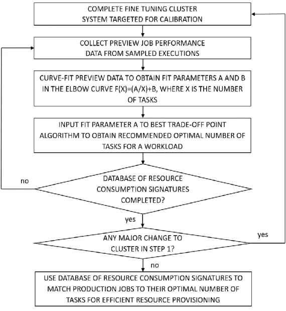
The Best Trade of Point (BToP) method provides an innovative approach and algorithm with mathematical formulas for finding an exact optimal number of computing resources for a workload as the best trade-off point between performance and resources on a runtime elbow curve fitted from sampled executions of the target cluster. The proposed techniques could be used in a large variety of systems and applications which utilize a trade-off curve as a powerful tool for making informed decisions. This thesis will focus on efficient resource provisioning in the two most prominent cluster-computing frameworks, Hadoop MapReduce and Apache Spark.The sequential steps for implementing the proposed BToP method on a cluster-computing system are as follows (Fig. 1):
1. Complete the configuration and fine tuning of the architecture, software and hardware of the production cluster-computing system targeted for calibration.
2. Collect necessary preview job performance data from historical runtime performances or sampled executions on the same target production system, configured exactly as in step 1, as reference points for each workload.
3. Curve-fit the preview data to obtain the fit parameters a and b in the runtime elbow curve function f(x)=(a/x)+b, where x is the number of task resources.
4. Input the fit parameter a to the Best Trade-off Point algorithm to obtain the recommended optimal number of tasks for a workload (Fig. 2-3).
a. The algorithm computes the number of tasks over a range of slopes from the first derivative of f(x)=(a/x)+b and the acceleration over a range of slopes from the second derivative of f(x)=(a/x)+b (Fig. 2-3).
7
b. The algorithm applies the Chain Rule to search for break points and major plateaus on the graphs of acceleration, slope, and task resources over a range of incremental changes in acceleration per slope increment (Fig. 2-3).
c. The algorithm extracts the exact number of tasks at the best trade-off point on the elbow curve and outputs it as recommended optimal number of tasks for a workload (Fig. 2-3).
5. Repeat steps 2-4 to gather sufficient resource provisioning data points for different workloads to build a database of resource consumption signatures for subsequent job profiling.
6. Repeat steps 1-5 to recalibrate the database of resource consumption signatures if there are any major changes to step 1.
8
7. Use the database of resource consumption signatures to match dynamically submitted production jobs to their recommended optimal number of tasks for efficient resource provisioning.
These steps for implementing the Best Trade-off Point algorithm for efficient resource provisioning could be also used with any other types of software components or data processing engines in the Hadoop ecosystem, any computing system, network data routing system, cluster microarchitecture system, payload engine system including but not limited to vehicle, aircraft/plane/jet, boat/ship, and rocket. This method could also be used with the yield curve of various types of securities, the convex iso yield curve, also known as convex isoquant curve, and the indifference curve in economics and manufacturing such as the semiconductor/IC yield curve, the manufacturing quality control curve, and any other types of trade-off curves with elbow shapes, both inverted or non-inverted, for making intelligent decisions. The isoquant analysis shows various combinations of factors of production that can produce a certain amount of output. In the convex isoquant curve, the factors can be substituted for each other only up to a certain extent. The proposed method can be used to determine the sweet spot on the elbow curve which is the best trade-off point between the factors.
In general, the proposed Best Trade-off Point method can be used in any other types of applications which rely on an elbow curve f(x)=(a/x)+b or an inverted elbow curve
f(x)=-(a/x)+b of performance vs. resources for good decision making including efficient resource provisioning. An elbow curve is a form of an exponential function with a negative growth rate. It is an exponential decay function f(x)=(a/x)+b where f(x) approaches b
instead of zero when x approaches infinity. On the other hand, an inverted elbow curve is a function with inverted exponential growth f(x)=-(a/x)+b where f(x) approaches b instead of infinity when x approaches infinity.
Typically, in Data Science applications, we could have an inverted elbow curve, also known as a knee curve (negative elbow curve), of performance vs. data where increasing the size of data no longer improves performance after a certain point. Thus, the BToP algorithm for an inverted elbow curve could simply be derived from the BToP algorithm for a non-inverted elbow curve as shown in Fig, 3. And the sequential steps of the BToP
9
method will still be the same with the exception that the elbow curve function is now inverted as f(x)=-(a/x)+b).
To illustrate another area of application of the proposed BToP method with an inverted elbow curve, we could consider a simplified example of determining the optimal travel speed for achieving the best miles-per-gallon (MPG) in fuel resource consumption on any individual fuel engine vehicle. There have been many suggestions that the travel speed for best MPG is within the range from 50 to 70 miles per hour. But there is yet a viable method for determining the exact optimal travel speed for best MPG, which varies from one car to another even on the same model. The optimal travel speed for best MPG depends on many factors and variables including but not limited to car model, engine size, car condition, engine tuning condition, tires, type of fuel, loads, route and weather condition, and so on, just to name a few. Using the proposed method and algorithm to
10
determine the Best Trade-off Point on an elbow curve of performance vs. resources, which is an inverted elbow curve of travel speed vs. fuel resources, in this case, the travel speed for best MPG could be accurately and precisely determined for every individual car.
The steps to Implement the Best Trade-off Point algorithm for efficient fuel resource provisioning in a fuel engine vehicle carrying a certain payload on a specific route and weather condition are basically the same as the ones for the application on a computer system. Following is the outline of sequential steps that a fuel engine system would perform to implement an embodiment of the proposed method.
1. Complete the tune-up of the fuel engine vehicle targeted for calibration.
2. Collect enough samples of speed performance vs. fuel resource consumption as preview data to plot the inverted elbow curve (knee curve) by running the car at different travel speeds on a specific route and weather condition and take measurements of the corresponding fuel consumption at those speeds. Each payload on a specific route and weather condition will have its own inverted elbow curve of speed performance vs fuel resources.
3. Curve-fitting the preview data to obtain the fit parameters a and b in the inverted elbow curve function f(x)=-(a/x)+b, where x is the number of fuel resources.
4. Input the fit parameter a to the Best-Trade-off-Point algorithm (Fig. 3) which is now modeled with f(x)=-(a/x)+b for an inverted elbow curve, to obtain the recommended optimal number of fuel resources for a payload on a specific route and weather condition. a. The algorithm computes the number of fuel resources over a range of slopes from the first derivative of f(x)=-(a/x)+b and the acceleration over a range of slopes from the second derivative of f(x)=-(a/x)+b.
b. The algorithm applies the Chain Rule to search for break points and major plateaus on the graphs of acceleration, slope, and fuel resources over a range of incremental changes in acceleration per slope increment.
11
c. The algorithm extracts the exact number of fuel resources at the best trade-off point on the inverted elbow curve and outputs it as recommended optimal number of fuel resources for a payload on a specific route and weather condition.
5. Repeat steps 2–4 to build a database of resource consumption signatures with different payloads on a specific route and weather condition for subsequent transportation job profiling.
6. If there is any major change to step 1, repeat steps 1–5 to recalibrate the database of resource consumption signatures.
7. Use the database of resource consumption signatures to match transportation jobs to their optimal number of fuel resources for efficient resource provisioning.
The crux of the proposed Best Trade-off Point method is not tied to any specific system. The Best Trade-off Point method provides a general approach and techniques based on an algorithm with mathematical formulas to find the best trade-off point on an elbow curve which is applicable to any system relying on a trade-off curve for making good decisions. As mentioned earlier, there are quite a few of applications and systems which are characterized by an elbow curve. The potential of commercializing the proposed method is huge since it touches every area of decision making process which relies on a trade-off curve for good decision making, including but not limited to efficient resource provisioning. Although the proposed method as presented in this thesis is used to optimize resource provisioning in Hadoop MapReduce and Apache Spark for performance efficiency, which often corresponds to energy efficiency, it is not limited to that software frameworks and hardware computing system. As clearly stated, the proposed method to find the best trade-off point for efficient resource provisioning is applicable whenever there is an elbow curve which is the fundamental trade-off curve. As such, the hardware that the invention could run on depends on the type of application which the Best Trade-off Point method is implemented on. As an example, for applications with runtime vs. resource trade-off curves, the hardware could be any computing systems including multicore systems, computer cluster, grid computers, network routers, and so on. For applications with trade-off curves of horse power, speed, travel distance, payload or weight vs. resource such as fuel or electricity, the hardware could be a car engine, jet engine, boat engine or
12
rocket. Not to mention for business applications with cost vs. quality control or delivery time, the underline hardware then becomes a manufacturing or production system.
13
Chapter 3
Efficient Resource Provisioning in
MapReduce
3.1 Pertinent Research in Performance Efficiency of MapReduce
Several research groups have worked on the performance and energy efficiency of Hadoop MapReduce. Krish et al. [26] present a workflow scheduler for MapReduce framework that profiles the performance and energy characteristics of applications on each hardware sub-cluster in a heterogeneous cluster to improve matching application to resource while ensuring energy efficiency and performance related Service Level Agreement goals. Hartog et al. [17] suggest a MapReduce framework configuration to evaluate node power consumption status and dynamically shift work toward more energy efficient node. Leverich and Kozyrakis [29] propose modifying Hadoop to allow the scaling down of operational clusters by keeping only a small fraction of the nodes running while disabling nodes not in the covering subset to conserve power. Lang and Patel [28] use all the nodes in the Hadoop cluster to run a workload and then power down the entire cluster when there is no work as an all-in-strategy. Kaushik and Bhandarkar [25] place classified data into two logical zones of HDFS, where 26% energy consumption reduction is achieved from cold zone power management, and there is room for further energy saving in the under-utilized hot zone. Lin et al. [30] analyze and derive the job energy consumption from the job completion reliability of the general MapReduce infrastructure based on a Poisson distribution to find way to achieve energy-efficient MapReduce environment. Wang et al. [38] use a genetic algorithm with practical encoding and decoding methods, and specially designed genetic operators to support a new MapReduce energy-efficient task scheduling model. Chen et al. [8] show that for MapReduce workloads, where the work rate is proportional to the amount of resources used, improving the performance as measured by traditional metrics such as job duration is equivalent to improving the performance as measured by lower energy consumed. For
14
most systems, decreasing energy consumption is equivalent to decreasing the finishing time.
Among the above research work dedicated to improving the energy efficiency of Hadoop MapReduce, we find that Chen et al. [8]’s publication is the most closely related to our work. Chen et al. [8] suggest a way to answer the question of how many machines to allocate to a particular job by comparing energy consumption of different numbers of machines but do not provide a method to find the exact optimal number. A smaller number of machines always consumes less energy, and takes longer to finish a job unless it has far exceeded the resources required for the job. In this thesis, we present a solution for finding the best trade-off point in performance and energy efficiency. We propose a general method, formula, and algorithm for obtaining the exact optimal number of tasks for any workload running on Hadoop MapReduce, to provision for performance efficiency based on the actual preview runtime data of the cluster targeted for calibration.
3.2 Background knowledge on MapReduce
Apache Hadoop [1, 39] is an open source framework for distributed storage and processing of large sets of data on clusters of commodity hardware. Although Hadoop ecosystem includes several software packages such as HBase, Hive, Mahout, Pig, Scoop, Spark, Storm and others, the base Apache Hadoop 2.0 framework comprises only four key modules: (1) Hadoop Common which provides file systems and OS level abstractions, (2) Hadoop Distributed File System (HDFS), (3) Hadoop YARN (Yet Another Resource
Negotiator) which manages computing resources in clusters and using them for scheduling of users’ apps, and (4) Hadoop MapReduce engine (MR2) which implements MR programming model (Fig. 8). With the addition of YARN in Hadoop 2.0, multiple applications while sharing a common cluster resource management can now be run in parallel by new engines. Hadoop clusters can now be scaled up to a much larger configuration and support iterative processing, graph processing, stream processing, and general cluster computing all at the same time.
15
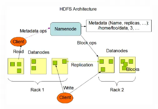
3.2.1 Hadoop Distributed File System (HDFS)
HDFS, which is based on Google File System (GFS), a master/slave architecture, supports large-scale data processing workloads and reliable data storage of several TB on clusters of commodity hardware (Fig. 4). It features high scalability, high availability, fault tolerance, flexible access, load balancing, tunable replication, and security. Since HDFS is designed more for batch processing rather than interactive use, it emphasizes more on high throughput of data than low latency of data access. HDFS has a simple coherency model: write-one-and-read-many access model, which supports appends and truncates only with no updates at arbitrary points. It is designed for high portability across heterogeneous hardware and software platforms.
Source: hadoop.apache.org Fig. 4 Architecture of Hadoop Distributed File System (HDFS)
HDFS splits files into default blocks of 64 MB or 128 MB, which are distributed among the nodes to provide a very high aggregate bandwidth across the cluster for compute performance and data protection. There is a single master called NameNode, which coordinates access and metadata as a simple centralized management system. There is no data caching error because the NameNode stores all metadata, which include filenames and locations of each file on DataNode, in memory for fast lookup. The DataNode only stores
16
blocks from files. NameNode makes all decisions regarding block replications. NameNode periodically receives a Heartbeat and a Blockreport from each DataNode. A secondary NameNode, running on a separate machine, periodically merges edit logs with namespace snapshot image stored on disk to prevent the edit log file from growing into a large file. In case of NameNode failure, the saved metadata can rebuild a failed primary NameNode with some data loss since the state of secondary NameNode always lags from the primary NameNode.
HDFS’s block replication feature is designed to tolerate frequent component failure and is optimized for huge number of very large files on up to several thousand nodes cluster, which are mostly read and appended. HDFS minimizes global bandwidth consumption and read latency with replica locality. Nodes are chosen based on rack-aware replica placement policy first, and then storage types and policies, to improve data reliability, availability, and network bandwidth utilization.
3.2.2 MapReduce Programming Model
The MapReduce programming model uses parallel and distributed algorithm on a cluster of nodes to process large datasets, unstructured as in a file system or structured as in a database. MapReduce can take advantage of data locality by passing data to each data node within the Hadoop cluster. MapReduce also packages users’ MapReduce functions as a Java ARchive (JAR) file and sends it out to each node. The JAR file operates locally on that slice of input on that data node and therefore, reduces the distance over which it must be transmitted. By executing compute at the location of data instead of having data moved to the compute location, traditional network bandwidth bottlenecks could be avoided. Moving computation to data is much more efficient than vice versa, The MapReduce framework provides scalability, security and authentication, resource management, optimized scheduling, flexibility, and high availability for a variety of applications in Big Data including but not limited to machine learning, financial analysis, genetic algorithms, natural language processing, signal processing, and simulation.
17
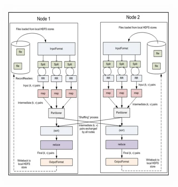
Source: Yahoo! Developer Network Fig. 5 MapReduce Data Flow
MapReduce consists of three phases, map, shuffle and reduce, where all values are processed independently. The reduce phase cannot start until the map phase is completely finished. At the map phase, map() functions run in parallel, creating different intermediate values from different input datasets: map(input_key, input_value) ->list <intermediate_key, intermediate_value>. At the shuffle phase after partitioning, values are
18
exchanged by a shuffle/combine process which runs on mapper nodes as a mini reduce phase on local map output to save bandwidth before sending data to full reducer. At the reduce phase, reduce() functions, also running in parallel, aggregate all values for a specific key to a single output to generate a new list of reduced output: list<intermediate_key, intermediate_value>->list<output_key, output_value> (Fig. 5).
3.2.3 MapReduce Job Execution on YARN
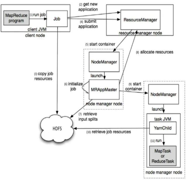
YARN splits the responsibilities of job tracker and task tracker in MapReduce v.1 into four separate entities in MapReduce v.2: (1) The ResourceManager has a built-in scheduler, which allocates resources across all applications based on the applications’ resource requirements. (2) The MR ApplicationMaster, which negotiates appropriate resource containers from the scheduler and tracks their progress, coordinates and manages each and every instance of MapReduce jobs executed on YARN. (3) The NodeManager, which is responsible for containers, monitors each and every node’s resource usage (CPU, memory, disk, network bandwidth) within YARN. (4) The Container allocates and represents resources per node available for each specific application (Fig.6). Thus, the tasks running MapReduce job is coordinated by the MR Application Master, which creates a map task object for each split and a number of reduce task objects determined by the mapreduce.job.reduces property.
The sequential steps of how Hadoop runs a MapReduce job using YARN are shown in Fig. 6. Step (1), a MapReduce job is submitted to a job client. Step (2), the job client requests for a new application ID from ResourceManager. Step (3), the job client checks HDFS to see whether an output has been created for that input and copy the result from HDFS directly if it exists. Otherwise, the job client copies job resources from HDFS. Step (4), the job is submitted to ResourceManager where a Scheduler allocates resources and an Application Manager monitors progress and status of the job. Step (5), ResourceManager contacts a NodeManager to start a new container and launch a MapReduce AppMaster for the job. Step (6), MR AppMaster creates an object for bookkeeping purpose and task management. Step (7), MR AppMaster retrieves the input splits from HDFS and creates a task for each split. Step (8), MR AppMaster decides how
19
Source: Hadoop: The Definitive Guide by Tom White (2012) Fig. 6 MapReduce Job Execution on YARN
to run the MapReduce task. Small jobs can be run on the same JVM on a single node as an Uber task. Large jobs request more resources to be allocated by ResourceManager which gathers information from the heartbeats of NodeManagers to consider data locality in its node allocation. Step (9), MR AppMaster contacts a NodeManager to start a new container for task execution. A YarnChild is launched to run on a separate JVM to isolate user codes from long running system deamons. Step (10), YarnChild retrieves job resources from HDFS. Step (11), YarnChild runs Map task or Reduce task. In every 3 secs, YarnChild sends a progress report to MR AppMaster which aggregates all reports and sends an update
20
directly to the job client. Upon job completion, MR AppMaster and task containers clean up their working states, and terminate themselves to release resources.
3.3. MapReduce Resource Provisioning
In general, allocating a higher number of tasks increases parallelization, framework overhead and load balancing, and minimizes the cost of failures to smaller increments of resources. But too many or too few tasks, whether mappers or reducers, are both detrimental for job performance. When the number of tasks is too large potentially causing resource contention and overall performance degradation, the overhead time spent by all task resources continues to grow while there is no further reduction in job runtime with the gradual increase in number of allocated tasks. When the number of tasks is too little for a workload, the job runtime is extremely high due to resource insufficiency (Fig. 7). Our goal is to find the best trade-off point between runtime and task resources to provision for optimal performance and energy efficiency.
There are some prior works on MapReduce resource provisioning to achieve certain application performance goals and Service Level Objectives (SLOs) which could be referenced when using our method for obtaining optimal task resources for energy efficient computing. Babu [6] suggests different techniques for automatic setting of job configuration parameters for MapReduce programs, including dynamic profiling, but acknowledges that this is an inherently difficult research and engineering challenge when the properties of the actual job being processed, its input data, and resource allocation are not known. Herodotou et al. [18] introduce the Elasticizer system to configure the right cluster size matching a workload’s performance needs by using an automated technique based on a mix of job profiling and simulation. Verma et al. [37] generate a set of resource provisioning options to meet given SLOs by applying scaling rules to the job past executions or sampled executions from a given application on the set of small input datasets. Kambatla et al. [22] propose a brute force job provisioning approach by analyzing and comparing the resource consumption of the application at hand with a database of similar resource consumption signatures of other applications to calculate the optimum configuration.
21
Fig. 7 Graphs of time spent by all map tasks, CPU, and Teragen execution versus number of launched map tasks. The runtime elbow curves of Teragen (a) 10 GB, (b) 100 GB and (c) 1 TB workloads plotted at different y-axis scales all appear to have the best trade-off points for performance efficiency at around 10 map tasks. But that is refuted by our algorithm as a visual misperception of different granularities at low magnification.
22
For the greater part, these prior research papers on resource provisioning for MapReduce v.1 are still applicable to MapReduce v.2. However, MapReduce v.2 is considerably different than MapReduce v.1, where there are pre-configured static slots for map and reduce tasks, which are inflexible and often leads to an under-utilization of resources. In YARN, the job tracker’s role of the previous MapReduce v.1 is now handled by a separate resource manager and history server to improve scalability. The NodeManager in MapReduce v.2, which manages resources and deployment on a node, is now responsible for launching containers. Each container can store a map or reduce task. MapReduce v.2 running on YARN is more scalable with resource utilization configured in terms of physical RAM limit, virtual memory and JVM heap size limit for each task. These improvements allow Hadoop to share resources dynamically between applications in a finer-grained, more practical and scalable resource configuration for better provisioning and cluster utilization. Along the lines proposed by these prior papers for resource provisioning by job profiles, our research paper further provides an innovative method, formula and algorithm to eliminate the guesswork, and accurately identify the optimal numbers of task resources for different workloads to achieve performance efficiency on any specific Hadoop cluster while minimizing any strenuous brute force.
Obtaining the optimal number of mappers and reducers for each job has been a challenge for Hadoop MapReduce users since there are lots of variables involved in balancing computing resources with network transfer bandwidth and disk reads. There are more than 180 parameters specified to control the behavior of a MapReduce job in Hadoop and the settings of more than 25 of these parameters can have significant impact on job performance [6, 22]. However, the optimal number of tasks for a job depends not only on the settings of various parameters and metrics for fine tuning Hadoop cluster performance but also on several other factors including but not limited to the type of application, dataset size and structure, cluster hardware specifications, system setup and configuration, and output buffer size. Therefore, the most practical method to indirectly take all those factors into account is to compute the optimal number of tasks from the actual sampled runtime data of the target cluster.
23
The number of maps needed for a certain job is usually decided by the number of blocks in the job inputs, which varies with the HDFS block size. The current default HDFS block size is 128 MB, an increase from the previous version, which was 64 MB. In some cases, capitalizing on data locality to enlarge the HDFS block size up to 512 MB to store a large input file can reduce the runtime for I/O bound jobs. On the other hand, when mappers are more CPU bound and less I/O bound, reducing the HDFS block size can improve the utilization of computing resources in the cluster. Hence, the total number of mappers running for a job depends on the number of input splits of the data. According to Hadoop Wiki, the right level of parallelism for maps seems to be around 10–100 maps/node, although it could be taken up to 300 or so for very CPU-light map tasks [16]. Significantly, the number of reducers at the aggregation step is more difficult to estimate since it is not easy to ascertain any spill of intermediate outputs to memory buffer and/or to disk for different workloads. Although there are currently three popular rules of thumb widely circulated in industry for deciding on the optimal number of reducers for a job, none of them provide an accurate and verifiable number of task resources for certain workload as shown in Fig. 17 in Section 3.6.
3.4. Best Trade-off Point (BToP) Algorithm for Optimal Resource Provisioning
We have developed an algorithm (Fig. 2-3) to search for the best trade-off points on the elbow curve of runtime versus number of launched tasks to overcome the uncertainty of all variables involved in finding the optimal number of tasks for a job to run in a specific Hadoop cluster. Before applying the algorithm, Hadoop users should first get some sampled executions from their target production system as reference points sufficient to plot a smooth elbow curve for each workload.
From the shape of the elbow curve of runtime versus task resources, we intuitively recognize its graph function f (x ) = ( a / x ) + b, which is confirmed by curve-fitting the preview data to obtain the fit parameters a and b. Using the fit parameter a as input, our program computes the number of tasks over a range of slopes from the first derivative and the acceleration over a range of slopes from the second derivative. Applying the Chain rule to our search algorithm for break points and major plateaus on the graphs of acceleration, slope, and task resources over a range of incremental changes in acceleration per slope
24
increment, our program extracts the exact number of tasks at the best trade-off point on the elbow curve and outputs it as recommended optimal number of tasks for a workload (Fig. 13-14 in Section 3.5.3).
This preview method, as job profiling for optimization of task resource provisioning, should work out well in any production environment where most of the jobs frequently submitted are of the same type of applications combined with different sizes of dataset. Hadoop users only need to calibrate the optimal numbers of tasks for each different workload in their production system once to build up a table of signatures and use them for all equivalent jobs. However, if there are subsequent changes made to the cluster’s system architecture, hardware setup, and configuration, a recalibration for a new set of optimal number of task resources might be necessary to maintain accuracy and precision. Once a database of signatures has been established, dynamically submitted jobs with different workloads can be quickly matched to their recommended optimal resource values for allocation using nested for-loops or equivalent structure to find resembling applications and datasets. The performance of task resources should be predictable through the job profiling of the same identical cluster-based system.
Therefore, it is possible to provide a single and general approach for automatic provisioning based on each specific system and application. However, users must establish a database of resource utilization signatures corresponding to workloads for every different application with various sizes of input datasets in advance. This approach relying on behavior replication is best suitable for production environment with repetitive workloads corresponding to the values of identical characteristics within the range of signatures pre-computed during a preview stage. It may be difficult and far less accurate to generally provision for a class of applications due to the diversified nature of MapReduce applications. Chen and Ganapathi et al. [7], in their development of an empirical workload model using production workload traces from Facebook and Yahoo to generate and replay synthetic workloads, acknowledge that per-workload performance measurements are necessary, and using proxy datasets and map/reduce functions can alter performance behavior considerably. In order to avoid recalibration of their workload model upon any change in the input data, map/reduce function code, or the underlying hardware/software
25
system, Chen and Ganapathi et al. [7] exclude system characteristics and system behavior from the workload description. Their method with replay mechanisms, which yield some useful insights by enabling performance comparisons across various system and workload changes, is in contrast with our general approach, which emphasizes on the accuracy of optimal resource provisioning for each application running on a specific system.
3.5 Design, Analysis, and Implementation of BToP Algorithm 3.5.1 Experimental background
To illustrate our method for obtaining the optimal number of task resources for different workloads, we use the Teragen and Terasort components of the Terasort benchmark test, which is part of the open source Apache Hadoop distribution, to experiment with 10 GB, 100 GB and 1 TB datasets. The benchmark tests are performed on a 24-node homogeneous Hadoop cluster, with two racks of 12 nodes each, running Cloudera CDH-5.2 YARN (MapReduce v.2). The NameNodes are VM (virtual machines) of 4 cores and 24 GB of RAM each running on Intel Xeon E5-2690 physical hosts of 8 cores and 16 threads with 2.9 GHz base frequency and 3.8 GHz max turbo frequency, and Thermal Design Power (TDP) of 135 W. The DataNodes/NodeManagers are physical system running Intel Xeon E3-1240 v.3 CPUs with 3.4 GHz base frequency and 3.8 GHz max turbo frequency, and TDP of 80 W. Each NodeManager has 4 cores, 8 threads, 32 GB of RAM, two 6 TB hard disks and 1Gbit network bandwidth. All nodes are connected to a switch with a backplane speed of 48 Gbps.
To sample executions of the Hadoop cluster under test, we use the
-Dmapreduce.job.maps = (int num) and -Dmapreduce.job.reduces = (int num) as a hint to the InputFormat to allocate the number of mappers and reducers during command line execution of JAR instead of setting the number of tasks in the code using the JobConf’s conf.setNumMapTasks (int num) and conf.setNumReduceTasks (int num). For Teragen, which uses MapReduce programming engine to break up the data to be sorted using a random sequence, we generate 10 GB, 100 GB and 1 TB of data with
-Dmapreduce.job.maps set equal to a few reference points between 1 and 96. For Terasort, which uses MapReduce programming engine to sample and sort the data created by Teragen, we sort 10 GB, 100 GB and 1 TB of data with -Dmapreduce.job.reduces set equal
26
to a few reference points between 1 and 96 (Fig. 8). We observe MapReduce’s behaviors in terms of total time spent by all map tasks, total time spent by all reduce tasks, CPU time spent by MapReduce framework, and the job execution time to develop a general formula for obtaining the optimal number of tasks for efficient use of available computing resources ( Fig. 9, Fig. 7, and Fig. 10).
27
28
Fig. 10 Graphs of time spent by all map tasks, all reduce tasks, CPU, and Terasort execution versus number of launched reduce tasks. The runtime elbow curves of Terasort (a) 10 GB, (b) 100 GB and (c) 1 TB workloads plotted at different y-axis scales all appear to have the best trade-off points for performance efficiency at around 10 reduce tasks. But that is disproved by our algorithm as a visual misperception of different granularities at low magnification.
29
3.5.2 Preview data
Although we performed thorough benchmark tests at numerous data points in our experiment, sampling around over a dozen points, which cover the whole elbow curve, will be sufficient to compute the target optimal task resource values. To get a little smoother graph, increase the number of points for the theoretical curve. Since the graphs of both Teragen and Terasort preview data are plotted at different vertical scales, where the 100 GB and 1 TB plots are around 10 to 100 times lower in magnification than the 10 GB plot, respectively (Fig. 7 and Fig. 10), it appears at first glance that there is no further significant improvement in runtime at the bottom of the elbow curves starting from around 10 launched map tasks and up for all three workloads. But that is a visual misperception of different granularities at low magnification since our algorithm shows that the best trade-off points are actually located at higher numbers of tasks, especially for large workloads.
In both component benchmark tests (Fig. 7 and Fig. 10), the CPU time spent by MapReduce framework increases with the number of task resources since there is more framework overhead. There is no plot of CPU time spent on reduce tasks in Teragen since it only breaks up the data to be sorted by Terasort and does not do any aggregation. For Terasort, we are only concerned about the time spent by all reduce tasks. We let mappers be allocated by MapReduce in Terasort based on the number of blocks in the input dataset previously generated by Teragen. The number of mappers for a given workload is driven by the number of input splits, and not by the -Dmapreduce.job.maps parameter set at the command line JAR execution. For each input split, a map task is spawned by MapReduce
framework. Thus, 80 mappers are spawned from 10 GB /
128 MB = 1 0∗1 0 2 4 MB/128 MB = 80 input splits for Terasort 10 GB, and that number increases to 800 and 8192 mappers for Terasort 100 GB and 1 TB, respectively.
As expected, the job execution time increases with larger workload and decreases with a higher number of launched tasks. However, assigning more tasks than necessary for a job will result in waste of computing resources since the reduction in execution time quickly decreases and becomes insignificant after the needed task resource value has been reached.
30
3.5.3 Process for Ascertaining Optimal Number of Tasks
The best trade-off point on the runtime elbow curve should be the location where no further significant decrease in execution time could be obtained by continuing to increase the number of launched tasks. Since the rate of descending of the execution time is the downhill slope of the graph, the target point could be found in the area where the slope is gentle and no longer steep, and the vertical movement has diminished close to almost flat. To find the slope, we take the derivative of the polynomial function
(1)
where x is the number of launched map tasks and launched reduced tasks for Teragen and Terasort, respectively. The derivative of f (x ) is a slope of a tangent line at a point x on a graph f (x ). It is equivalent to the slope of a secant line between two points x
and on the graph, where approaches 0.
(2) From (1),
f′( x ) = − a x− 2 (3)
and therefore,
(4)
where f′(x )< 0 for a downhill slope with a negative value.
Using GNUplot to curve-fit the preview data points, we obtain the fit parameters a and b of the graph function f (x ) = (a / x ) + b ( F i g. 1 1 ) . GNUplot fit command uses Levenberg–Marquardt Algorithm (LMA), also known as the damped least-squares (DLS) method, which is used to solve non-linear least least-squares problems. LMA interpolates between the Gauss–Newton algorithm (GNA) and the method of gradient descent. However, LMA is more robust than the Gauss-Neuton algorithm since, in many cases, it could find a solution even if it starts very far off the final minimum. The GNUplot
31
Fig. 11 Fitting Teragen preview data using Levenberg–Marquardt Algorithm (LMA), aka the damped least-squares (DLS) method.
32
fit command is used to find a set of parameters that best fits the input data to the user-defined function, which is f(x)=(a/x)+b here. The fit is judged based on the Sum of Squared Residuals (SSR) between the input data and the function values, evaluated at the same places on the curve. LMA will try to minimize the weighted SSR or chisquare. A reduced chisquare much larger than 1.0 may be caused by incorrect data error estimates, data errors not normally distributed, systematic measurement errors, 'outliers', or an incorrect model function. The parameter error estimates, which are readily obtained from the variance-covariance matrix after the final iteration, is reported as "asymptotic standard errors".
Using the obtained fit parameter a, we then plot the three fitted elbow curves of execution time versus launched task resources for Teragen and Terasort 10 GB, 100 GB and 1 TB workloads (Fig. 12).
Taking the second derivative of the function f (x ), which is the derivative of the slope, we have the acceleration of the rate of change in number of task resources:
f″( x ) = f′( f′( x ) ) (5)
(6)
(7) as the second symmetric derivative.
From (2),
f″( x ) = 2 a x− 3 (8)
Our algorithm finds the optimal number of tasks recommended for a workload by locating the best trade-off point at the bottom of the elbow curve where assigning more task resources no longer significantly reduces the job execution time and therefore, reduces the overall system efficiency in resource utilization and energy consumption. Taking the
33
Fig. 12 Fitted runtime elbow curves of (a) Teragen and (b) Terasort 10 GB, 100 GB, and 1 TB workloads versus number of launched map/reduce tasks, and their fit parameters a and b in the graph function f (x ) = ( a / x ) + b.
34
parameter a in f (x ) = (a / x )+ b as input, our program computes and tabulates the number of tasks over a range of slopes from −0.25 to −39.25 for , and the
acceleration over a range of slopes from −0.25 to −39.25 for .
Applying the Chain Rule
(9)
the rate of change in acceleration with respect to tasks is
(10)
Our algorithm looks for break points on the graphs to compute a table of recommended acceleration, corresponding slope, and optimal number of tasks, when the change in acceleration in the current slope increment is greater than or equal to the target value of change in acceleration per slope increment, and the change in acceleration in the next slope increment is less than the target value of change in acceleration per slope increment (Fig. 2-3, Fig. 13 and Fig. 15). Finally, our algorithm searches for all major plateaus lasting at least eight increments of change in acceleration on the graph of task resources versus change in acceleration per slope increment, which corresponds to the graph of slope versus change in acceleration per slope increment and the graph of acceleration versus change in acceleration per slope increment (Fig. 14 and Fig. 16). Our program then outputs the exact optimal numbers of tasks recommended for different workloads (Fig. 13 and Fig. 15). The first recommended number of tasks for the same workload provides the highest efficiency in system performance and energy consumption ratio. The subsequent recommended number(s) of tasks lowers the job runtime a little bit more but at a much less efficient performance/energy ratio. However, increasing the number of tasks beyond the recommended range does not necessarily translate into any further performance gain in execution time.
35
Fig. 13 Applying BToP algorithm to Teragen 10 GB, 100 GB, and 1 TB workloads, our program tabulates the number of tasks over range of slopes, acceleration over range of slopes, and recommended acceleration, slope, and optimal number of tasks over range of incremental changes in acceleration per slope increment, to output the final recommended optimal numbers of tasks for each Teragen workload.
36
Fig. 14 The optimal number of tasks for Teragen 10 GB, 100 GB, and 1 TB workloads are identified by the major plateaus lasting at least eight increments on the graphs. The algorithm searches for break points in the changes in acceleration and outputs: (a) recommended acceleration, (b) corresponding slope and (c) task resources versus change in acceleration per slope increment.
37
Fig. 15 Applying BToP algorithm to MR Terasort 10 GB, 100 GB, and 1 TB workloads, our program tabulates the number of tasks over range of slopes, acceleration over range of slopes, and recommended acceleration, slope, and optimal number of tasks over range of incremental changes in acceleration per slope increment, to output the final recommended optimal numbers of tasks for each Terasort workload.
38
Fig. 16 The optimal numbers of tasks for Terasort 10 GB, 100 GB, and 1 TB workloads are identified by the major plateaus lasting at least eight increments on the graphs. The algorithm searches for break points in the changes in acceleration and outputs: (a) recommended acceleration, (b) corresponding slope and (c) task resources versus change in acceleration per slope increment.