Uncovering Nonlinear Dynamics—The Case
Study of Sea Clutter
SIMON HAYKIN, FELLOW, IEEE, REMBRANDT BAKKER,
ANDBRIAN W. CURRIE
Invited Paper
Nonlinear dynamics are basic to the characterization of many physical phenomena encountered in practice. Typically, we are given a time series of some observable(s) and the requirement is to uncover the underlying dynamics responsible for generating the time series. This problem becomes particularly challenging when the process and measurement equations of the dynamics are both nonlinear and noisy. Such a problem is exemplified by the case study of sea clutter, which refers to radar backscatter from an ocean surface. After setting the stage for this case study, the paper presents tutorial reviews of: 1) the classical models of sea clutter based on the compoundK distribution and 2) the application of chaos theory to sea clutter. Experimental results are presented that cast doubts on chaos as a possible nonlinear dynamical mechanism for the generation of sea clutter. Most importantly, experimental results show that on timescales smaller than a few seconds, sea clutter is very well described as a complex autoregressive process of order four or five. On larger timescales, gravity or swell waves cause this process to be modulated in both amplitude and frequency. It is shown that the amount of frequency modulation is correlated with the nonlinearity of the clutter signal. The dynamical model is an important step forward from the classical statistical approaches, but it is in its early stages of development.
Keywords—Chaos, complex autoregressive models, compound
K-distribution, modulation, nonlinear dynamics, radar, sea clutter, short-time Fourier-transform, time-Doppler.
I. INTRODUCTION
Nonlinear dynamics are basic to the characterization of many physical phenomena encountered in practice. Typically, we are given a time series of some observable(s) and the requirement is to uncover the underlying dynamics responsible for generating the time series. In a fundamental sense, the dynamics of a system are governed by a pair of nonlinear equations.
Manuscript received July 27, 2001; revised November 14, 2001. This work was supported by the Natural Sciences and Engineering Research Council of Canada.
The authors are with McMaster University, Hamilton, ON L8S 4L7 Canada.
Publisher Item Identifier S 0018-9219(02)05240-4.
1) A recursive process equation, which describes the evo-lution of the hidden state vector of the system with time (1) where the vector is the state at discrete time is the dynamical or process noise, and is a vector-valued nonlinear function.
2) A measurement equation, which describes the depen-dence of observations (i.e., measurable variables) on the state
(2) where is the observation (assumed to be scalar), is the measurement noise, and is a nonlinear function.
The explicit dependence of both nonlinear functions and on time emphasizes the time-varying nature of the dynam-ical system.
Equations (1) and (2) define the state-space model of a nonlinear time-varying dynamical system in its most general form. The exact form of the model adopted in practice is influenced by two perspectives that are in a state of “tension” with each other:
1) mathematical tractability; 2) physical considerations.
Mathematical tractability is at its easiest when the system is linear and the dynamical noise and measurement noise are both additive and modeled as independent white Gaussian noise processes. Under this special set of conditions, the solution to the problem of uncovering the un-derlying dynamics of the system is to be found in the cele-brated Kalman filter [1]. In a very clever way, the Kalman filter solves the problem by exploiting the fact that there is a one-to-one correspondence between the given sequence of observable samples and the sequence of innovations derived from one-step predictions of the observables. The innovation
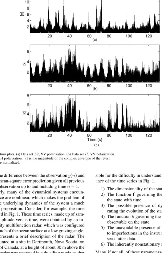
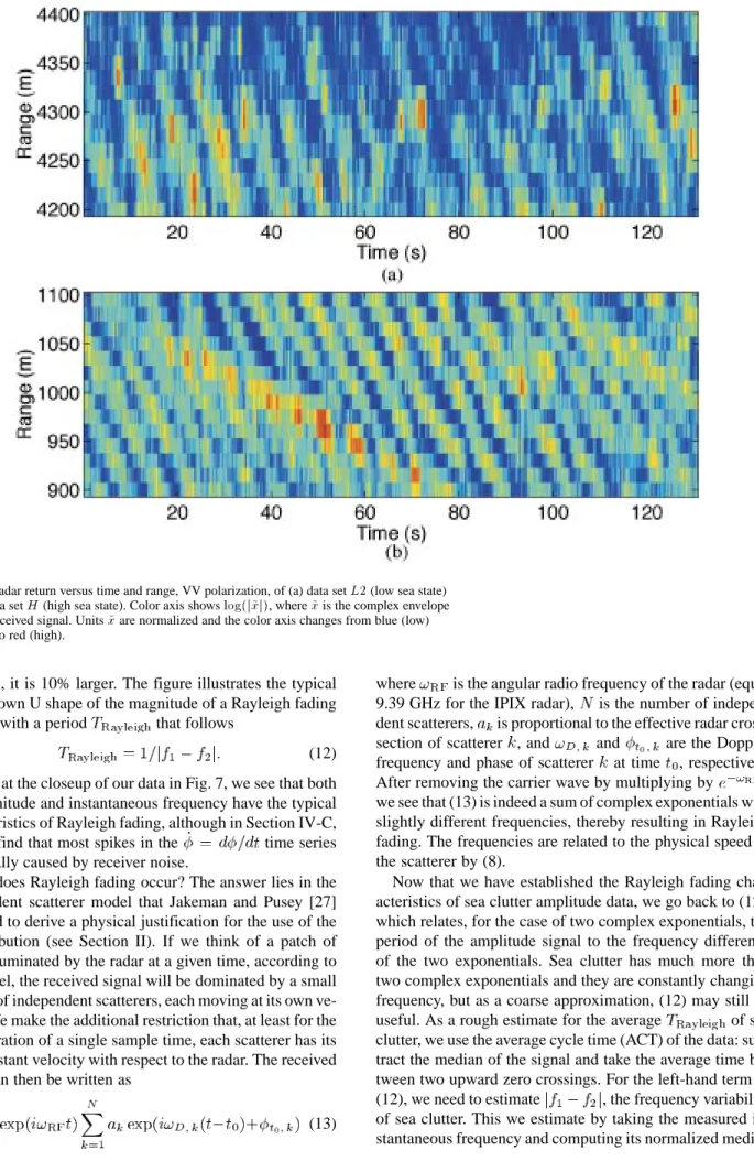
Fig. 1. Radar return plots. (a) Data setL2, VV polarization. (b) Data set H, VV polarization. (c) Data setH, HH polarization. jxj is the magnitude of the complex envelope of the return signal. Unitsx are normalized.
is defined as the difference between the observation and its minimum mean-square error prediction given all previous values of the observation up to and including time .
Unfortunately, many of the dynamical systems encoun-tered in practice are nonlinear, which makes the problem of uncovering the underlying dynamics of the system a much more difficult proposition. Consider, for example, the time series displayed in Fig. 1. These time series, made up of sam-pled signal amplitude versus time, were obtained by an in-strument-quality multifunction radar, which was configured to monitor a patch of the ocean surface at a low grazing angle. Appendix A presents a brief description of the radar. The radar was mounted at a site in Dartmouth, Nova Scotia, on the east coast of Canada, at a height of about 30 m above the sea level. The radar was operated in a dwelling mode so that the dynamics of the sea clutter (i.e., radar backscatter from the ocean surface) recorded by the radar would be entirely due to the motion of the ocean waves and the natural motion of the sea surface itself. Throughout the paper, we will make extensive use of three different data sets. Two data sets were measured at low wave-height conditions (0.8 m) and are la-beled and . For the third data set, labeled , the wave height was higher (1.8 m); the characteristics of these data sets are summarized in Appendix B.
From the viewpoint of dynamical systems as characterized by (1) and (2), we may identify six potential sources
respon-sible for the difficulty in understanding the complex appear-ance of the time series in Fig. 1.
1) The dimensionality of the state.
2) The function governing the nonlinear evolution of the state with time.
3) The possible presence of dynamical noise compli-cating the evolution of the state with time.
4) The function governing the dependence of the radar observable on the state.
5) The unavoidable presence of measurement noise due to imperfections in the instruments used to record the sea-clutter data.
6) The inherently nonstationary nature of sea clutter. Many, if not all, of these parameters/processes are unknown, which makes the uncovering of the underlying dynamics of sea clutter into a challenging task.
Random-looking time series, such as those of Fig. 1, can be modeled at various levels of sophistication. The crudest form is to look at the probability density function (pdf) of the data, ignoring any type of correlation in time. At the next level, correlations in time are modeled by a linear or higher order relationship and the residuals are described by their pdf. A third level of sophistication is sometimes possible for systems that exhibit low-dimensional dynamics [2]–[7]. For a subset of these systems, namely, deterministic chaotic
systems, the time series can be described completely in terms of nonlinear evolutions and, assuming a perfect model and noise-free measurements, there are no residuals at all. The deterministic chaos approach has enormous potential in that it makes it possible to reproduce the mechanism underlying the experimental data with a computer model. It has attracted the attention of numerous researchers in the natural and applied sciences, trying to identify if their data are close to being chaotic and lend themselves for a deterministic modeling approach. Chaos theory itself is motivated by earlier works of Kaplan and Yorke [8], Packard et al. [9], Takens [10], Mañé [11], Grassberger and Procaccia [12], Ruelle [13], Wolf et al. [14], Broomhead and King [15], Sauer et al. [16], Sidorowich [17], and Casdagli [18]. Indeed, these papers aroused interest in deterministic chaos as a possible mechanism for explaining the underlying dynamics of sea clutter [19]–[23]. Unfortunately, for reasons that will be explained later in Section III, currently available state-of-the-art algorithms used to estimate the chaotic invariants of sea clutter produce inconclusive results, which cast serious doubts on deterministic chaos as a possible mathematical basis for the nonlinear dynamics of sea clutter. This conclusion has been reinforced further by the inability to design a reliable algorithm for the dynamic reconstruction of sea clutter.
All along, our own primary research interests in sea clutter have been driven by the following issues of compelling prac-tical importance.
1) Sea clutter is a nonlinear dynamical process with time playing a critical role in its characterization. By con-trast, much of the effort devoted to the characterization of sea clutter during the past 50 years has focused on the statistics of sea clutter, with little attention given to time [24]–[30], other than adapting to time-varying statistical parameters.
2) Understanding the nonlinear dynamics of sea clutter is not only important in its own right, but it will have a significant impact on the joint detection and tracking of a point target on or near the sea surface. Such targets include low-flying aircraft, small marine vessels, and floating hazards, e.g., ice.
3) Identifying the particular part of the expanding litera-ture on nonlinear dynamics, which is applicable to re-liable characterization of sea clutter.
This paper is written with these objectives in mind, given what we currently know about the statistics and dynamics of sea clutter.
The rest of the paper is organized as follows. Section II presents a tutorial review of the classical models of sea clutter, with primary emphasis on the compound distribu-tion. Section III presents a critical review of results reported in the literature on the application of deterministic chaos analysis to sea clutter. The discussion presented therein concludes that the discovery that a real-world experimental time series is chaotic has a high risk of being a self-fulfilling prophecy. We justify this statement by revisiting earlier claims that sea clutter is the result of a deterministic chaotic
process. In Section IV, we go back to first principles in modulation theory and present new experimental results demonstrating that sea clutter is the result of a hybrid con-tinuous-wave modulation process that involves amplitude as well as frequency modulation; this section also includes a time-varying data-dependent autoregressive (AR) model for sea clutter, which, in a way, relates to our earlier work on the AR modeling of radar clutter in an air-traffic control environment [31]–[34]. Section V, the final section of the paper, presents conclusions and an overview of the current directions of research on recursive learning models that may be relevant to the nonlinear dynamics of sea clutter.
II. STATISTICALNATURE OFSEACLUTTER—CLASSICAL APPROACH
Sea clutter, referring to the radar backscatter from the sea surface, has a long history of being modeled as a stochastic process, which goes back to the early work of Goldstein [24]. One of the main reasons for this approach has been the random-looking behavior of the sea-clutter waveform. In the classical view, going back to Boltzmann, the irregular be-havior of a physical process encountered in nature is believed to be due to the interaction of a large number of degrees of freedom in the system. Hence, the justification for the statis-tical approach.
There are three signal domains of the radar waveform in which the clutter properties need to be characterized: 1) am-plitude; 2) phase; and 3) polarization. Noncoherent radars measure only the envelope (amplitude) of the clutter signal. Coherent radars are able to measure both signal amplitude and phase. Polarimetric effects are evident in both types of radar. Before discussing these effects, some background on the characterization of the sea surface and consideration of the geometry of a low-grazing angle radar is desirable. A. Background
It is the nature of the surface roughness that determines the properties of the radar echo [35]. The roughness of the sea surface is normally characterized in terms of two funda-mental types of waves. The first type is termed gravity waves, with wavelengths ranging from a few hundred meters to less than a meter. The dominant restoring force for these waves is the force of gravity. The second type is smaller capillary waves with wavelengths on the order of centimeters or less. The dominant restoring force for these waves is surface ten-sion.
The gravity waves, which describe the macrostructure of the sea surface, can be further subdivided into sea and swell. Sea consists of wind waves: steep short-crested waves driven by the winds in their locale. Swell consists of waves of long wavelength, nearly sinusoidal in shape, produced by distant winds. The very irregular appearance of the sea surface is due to interference of the various wind and swell waves and to local atmospheric turbulence. Near coastlines, ocean currents (usually tidal currents) may cause a considerable increase in the wave heights due to their interference with wind and
swell waves. The microstructure of the sea surface—the cap-illary waves—are usually caused by turbulent gusts of wind near the surface.
Waves are primarily characterized by their length, height, and period. The phase speed is the ratio of wave length over wave period. Wavelength and period (hence, phase speed) can be derived from the dispersion relation [36]. Wave height fluctuates considerably. A commonly reported measure is significant wave height, defined as the average peak-to-trough height of the one-third highest waves. It indicates the predominant wave height.
To provide a simple metric to indicate qualitatively the current sea conditions, the concept of the sea-state was introduced in [35, Table 2-1]. The sea-state links expected wave parameters, such as height and period, to environ-mental factors including wind speed, duration, and fetch. The frequently used short form gives the sea-state number only.
The angle at which the radar beam illuminates the sur-face is called the grazing angle , measured with respect to the local horizontal. The smallest area of the sea surface within which individual targets can no longer be individually resolved is termed the resolution cell, whose area is given by
sec (3)
where is range, is the azimuthal beamwidth of the an-tenna, is the speed of light, is the radar pulse length, and
is the grazing angle.
The backscatter power (square of the amplitude) has been studied at two different time scales. Studies [37] have pro-duced empirical models, relating the long-term (over several minutes) average to various parameters, including grazing angle, radar frequency and polarization, and wind and wave conditions.
1) Polarimetric Effects: One of the dominant scattering mechanisms at microwave frequencies and low-to-medium grazing angles is Bragg scattering. It is based on the prin-ciple that the returned signals from scatterers that are half a radar wavelength apart (measured along the line of sight from the radar) reinforce each other since they are in phase. At microwave frequencies, the Bragg scatter is from capillary waves. It has long been observed that there is a difference in the behavior of sea backscatter depending on the transmit polarization.1 Horizontally polarized (HH) backscatter has
a lower average power as compared to the vertically polar-ized (VV) backscatter, as predicted by the composite surface theory and Bragg scattering [38]. As a consequence, most marine radars operate with HH polarization. However, the HH signal often exhibits large target-like spikes in amplitude, with these spikes having decorrelation times on the order of one second or more.
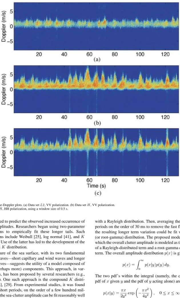
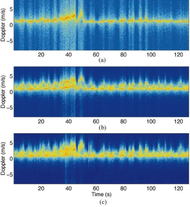
Fig. 2 shows the evolution of the Doppler spectrum versus time for the coherent data used to generate the amplitude plots of Fig. 1. In this case of incoming waves, the HH
spec-1A signal’s polarization is designated by a two-letter combinationT R,
whereT is the transmitted polarization (H or V) and R is the received po-larization (H or V).
trum on average is shifted further from the frequency origin (i.e., has a higher mean Doppler frequency) and, at the times of strong signal content, the HH spectrum may reach higher frequencies than does the VV spectrum.
The differences in the spectra suggest that different scatterers are contributing to the HH and VV returns. They can be partially explained from conditions associated with breaking waves. The breaking waves contribute to the bunching of scatterers, consistent with arguments for the applicability of the compound distribution [39]. With the scatterers bunched at or near the crest of the breaking wave, there is the opportunity for a multipath reflection from the sea surface in front of the wave. The polarization dependence arises from the relative phase of the direct and surface-reflected paths. For VV polarization, the Brewster effect may lead to strong cancellation of the return, whereas the HH polarization will exhibit a strong (possibly spiky) return [39]. The Brewster angle is the particular angle of incidence for which there is no reflected wave when the incident wave is vertically polarized.
From -band scatterometer data from advancing waves, Lee et al. [40] identified VV-dominant comparatively short-lived “slow (velocity) scatterers” and HH-dominant longer lived “fast (velocity) scatterers.” Because the water particles which define a breaking wave crest necessarily exceed the orbital acceleration of the linear-wave group that initiates the nonlinear evolution of the wave structure, the fact that fast scatterers are observed is not surprising. Sea spikes from advancing waves are collocated with the fastest scatterers, which are identified with the wave crest. Based on experi-mental data for approaching waves, Rino and Ngo [39] sug-gest that the VV backscatter is responding to slower scat-terers confined to the back side of the wave while HH is sponding to the fast scatterers near the wave crest. The HH re-sponse to the back-side scatterers (presumed to be Bragg-like structures) may be suppressed due to the angular dependence of the Bragg scattering.
B. Current Models
There are two goals related to the modeling of clutter. The first goal is to develop an explanation for the observed be-havior of sea clutter and, in so doing, to gain insight into the physical and electromagnetic factors that play a role in forming the clutter signal. Based on the success of the first goal, the second goal is to produce a model, ideally phys-ically based, with which a representative clutter signal can be generated, to extend receiver algorithm testing into clutter conditions for which sufficient real data are unavailable. Two current models that seek to address the second goal (at least in one of the signal domains) are the compound -distribu-tion model and the Doppler spectrum model.
1) Compound Distribution: Characterization of the amplitude fluctuations of the sea backscatter signal is a continuing source of study. Much of the early work in fitting amplitude distributions was based on the use of a Gaussian model, implying Rayleigh distributed amplitudes. However, it was soon found that operating with increased radar resolution and at low grazing angles, the Gaussian
Fig. 2. Time-Doppler plots. (a) Data setL2, VV polarization. (b) Data set H, VV polarization. (c) Data setH, HH polarization, using a window size of 0.5 s.
model failed to predict the observed increased occurrence of higher amplitudes. Researchers began using two-parameter distributions to empirically fit these longer tails. Such distributions include Weibull [25], log normal [41], and [29], [30]. Use of the latter has led to the development of the compound distribution.
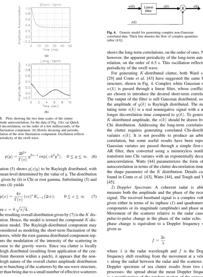
The nature of the sea surface, with its two fundamental types of waves—short capillary and wind waves and longer gravity waves—suggests the utility of a model composed of two (or perhaps more) components. This approach, in var-ious forms, has been proposed by several researchers (e.g., [28], [42]). One such approach is the compound distri-bution [28], [29]. From experimental studies, it was found that over short periods, on the order of a few hundred mil-liseconds, the sea-clutter amplitude can be fit reasonably well
with a Rayleigh distribution. Then, averaging the data over periods on the order of 30 ms to remove the fast fluctuation, the resulting longer term variation could be fit with a Chi (or root-gamma) distribution. The proposed model is one in which the overall clutter amplitude is modeled as the product of a Rayleigh-distributed term and a root-gamma distributed term. The overall amplitude distribution is given by
(4) The two pdf’s within the integral (namely, the conditional pdf of given and the pdf of acting alone) are
(a)
(b)
Fig. 3. Plots showing the two time scales of the clutter amplitude autocorrelation, for the data of Fig. 1(b). (a) Quick initial decorrelation, on the order of a few milliseconds, of the fast fluctuation component. (b) Slowly decaying and periodic correlation of the slow fluctuation component. Oscillation reflects the periodicity of the swell wave.
and
(6) Equation (5) shows to be Rayleigh distributed, with the mean level determined by the value of . The distribution of given by (6) is Chi or root gamma. Substituting (5) and (6) into (4) yields
(7)
where .
The resulting overall distribution given by (7) is the dis-tribution. Hence, the model is termed the compound -dis-tribution model. The Rayleigh-distributed component may be considered as modeling the short-term fluctuation of the scatterers, while the root-gamma distributed component rep-resents the modulation of the intensity of the scattering in response to the gravity waves. Since sea clutter is locally Rayleigh distributed (resulting from application of the cen-tral limit theorem within a patch), it appears that the non-Rayleigh nature of the overall clutter amplitude distribution is due to bunching of the scatterers by the sea wave structure, rather than being due to a small number of effective scatterers [29].
We need to consider the correlation properties of the clutter amplitude. Fig. 3 shows a typical plot of the autocor-relation of the VV signal on two time scales. Fig. 3(a), based on a sample period of 1 ms, shows that the correlation due to the fast fluctuation component is under 10 ms. Fig. 3(b)
Fig. 4. Generic model for generating complex non-Gaussian correlated data. Thick line denotes the flow of complex quantities (after [43]).
shows the long-term correlations, on the order of ones. Note, however, the apparent periodicity of the long-term autocor-relation, on the order of 6.5 s. This oscillation reflects the periodicity of the swell wave.
For generating -distributed clutter, both Ward et al. [29] and Conte et al. [43] have suggested the same basic structure, shown in Fig. 4. Complex white Gaussian noise is passed through a linear filter, whose coefficients are chosen to introduce the desired short-term correlation. The output of the filter is still Gaussian distributed, so that the amplitude of is Rayleigh distributed. The modu-lating term is a real nonnegative signal with a much longer decorrelation time compared to . To generate a -distributed amplitude, the should be drawn from a Chi distribution. Addressing the long-term correlation of the clutter requires generating correlated Chi-distributed variates . It is not possible to produce an arbitrary correlation, but some useful results have been reported. Gaussian variates are passed through a simple first-order AR filter, then converted using a memoryless nonlinear transform into Chi variates with an exponentially decaying autocorrelation. Watts [44] parameterizes the form of the autocorrelation in terms of the clutter decorrelation time and the shape parameter of the distribution. Details can be found in Conte et al. [43], Watts [44], and Tough and Ward [45].
2) Doppler Spectrum: A coherent radar is able to measure both the amplitude and the phase of the received signal. The received baseband signal is a complex voltage, given either in terms of its inphase ( ) and quadrature ( ) components or its magnitude (amplitude) and phase angle. Movement of the scatterer relative to the radar causes a pulse-to-pulse change in the phase of the radar echo. This phase change is equivalent to a Doppler frequency shift, given as
(8) where is the radar wavelength and is the Doppler frequency shift resulting from the movement at a velocity along the radial between the radar and the scatterer. The Doppler spectrum of sea clutter results from two main processes: the spread about the mean Doppler frequency is a manifestation of the random motion of the unresolved scatterers, while the displacement of the mean Doppler fre-quency maps the evolution of the resolved waves. Tracking the evolution of the Doppler spectrum versus time can provide insight into the scattering mechanisms and identify properties that a sea-clutter model should possess.
Note that in a realistic sea surface scenario, there will be a continuum of waves of various heights, lengths, and direc-tions. This continuum is typically characterized by a wave frequency spectrum (or wave-height spectrum), describing the distribution of wave height versus wave frequency. There are a number of models relating environmental parameters such as wind speed to the frequency spectrum [46]. The quency spectrum can then be extended to the directional fre-quency spectrum by introducing a directional distribution [47]. Under the assumption of linearity, the combined effect is the superposition of all the waves, calculated by integrating across the appropriate range of directional wave numbers. In reality, the final surface is a nonlinear combination of the continuum of waves.
Walker [48] studied the development of the Doppler spectra for HH and VV polarizations as breaking waves passed the radar sampling area. Coincident video images were taken of the physical wave. Three types of scattering regimes appear to be important: Bragg, whitecap, and spike events. Walker [49] proposes a three-component model for the Doppler spectrum based on these regimes.
1) Bragg Scattering: This regime makes VV amplitude greater than HH. Both polarizations peak at a
fre-quency corresponding to the velocity ,
where is the term attributable to the Bragg scat-terers and is a term encompassing the drift and orbital velocities of the underlying gravity waves. The decorrelation times of the two polarizations are short (tens of millseconds).
2) Whitecap Scattering: The backscatter amplitudes of the two polarizations are roughly equal and are notice-ably stronger than the background Bragg scatter, par-ticularly in HH, in which Bragg scattering is weak. In a time profile, the events may be seen to last for times on the order of seconds, but are noisy in structure and decorrelate quickly (again, in milliseconds). Doppler spectra are broad and centered at a speed noticeably higher than the Bragg speed, at or around the phase speed of the larger gravity waves.
3) Spikes: Spikes are strong in HH, but virtually absent in VV, with a Doppler shift higher than the Bragg shift. They last for a much shorter time than the whitecap returns (on the order of 0.1 s), but remain coherent over that time.
Each of these three regimes is assigned a Gaussian line shape, with three parameters: 1) its power (radar cross-sec-tion); 2) center frequency; and 3) frequency width. Assuming the overall spectrum is a linear combination of its compo-nents, the VV spectrum is the sum of Bragg and Whitecap lineshapes, while the HH spectrum is the sum of Bragg, Whitecap, and Spike lineshapes.
The model has been validated with experimental cliff-top radar data, for which the widths and relative amplitudes of the Gaussian lineshapes were determined using a minimization algorithm.
Other researchers have similarly identified Bragg and faster-than-Bragg components, using Gaussian lineshapes for the former, and Lorentzian and/or Voigtian lineshapes
for the latter [40]. The results were reported for the case of breaking waves but in the absence of wind.
In this section, we have focused on the classical statistical approach for the characterization of sea clutter. In the next section, we consider deterministic chaos as a possible mech-anism for the nonlinear dynamics of sea clutter.
III. ISTHERE ARADARCLUTTERATTRACTOR?
The Navier–Stokes dynamical equations are basic to the understanding of the underlying principles of fluid mechanics, including ocean physics [50]. Starting with these equations, Lorenz [51] derived an unrealistically simple model for atmospheric turbulence, which is described by three coupled nonlinear differential equations. The model, bearing his name, was obtained by deleting everything from the Navier–Stokes equations that appeared to be extraneous to the simplest mathematical description of the model. The three equations, governing the evolution of the Lorenz model, are deceptively simple, but the presence of certain nonlinear terms in all three equations gives rise to two unusual characteristics:
1) a fractal dimension equal to 2.01;
2) sensitivity to initial conditions, meaning that a very small perturbation in initialization of the model results in a significant deviation in the model’s trajectory in a relatively short interval of time.
These two properties are the hallmark of chaos [52], a sub-ject that has captured the interests of applied mathematicians, physicists, and, to a much lesser extent, signal-processing re-searchers during the past two decades.
A. Nonlinear Dynamics
Before anything else, for a process to qualify as a chaotic process, its underlying dynamics must be nonlinear. One test that we can use to check for the nonlinearity of an experimental time series is to employ surrogate data analysis [53]. The surrogate data are generated by using a stochastic linear model with the same autocorrelation function or, equivalently, power spectrum as the given time series. The exponential growth of interpoint distances between these two models is then used as the discriminating statistic to test the null hypothesis that the experimental time series can be described by linearly correlated noise. For this purpose, the Mann–Whitney rank-sum statistic, denoted by the symbol , is calculated. The statistic is Gaussian distributed with zero mean and unit variance under the null hypothesis that two observed samples of interpoint distances calculated for the experimental time series and the surrogate time series come from the same population. A value of less than 3.0 is considered to be a solid reason for strong rejection of the null hypothesis, i.e., the experimental time series is nonlinear [54].
Appendix B summarizes three real-life sea-clutter data sets, which were collected with the IPIX radar on the east coast of Canada. (A brief description of the IPIX radar is
presented in Appendix A.) Specifically, the data sets used in the case study are as follows.
1) Data set , corresponding to a lower sea state, with the ocean waves moving away from the radar. The sampling frequency of this data set is twice that of the other two data sets and .
2) Data set , corresponding to a higher sea state, with the ocean waves coming toward the radar.
3) Data set , corresponding to a lower sea state, taken earlier the same day as data set and at a radar range of 4 km compared to 1.2 km for data set . This differ-ence in range causes to have a considerably better signal-to-noise ratio (SNR) than .
Two different types of surrogate data were generated.
1) Data sets , and , which were
de-rived from sea clutter data sets , , and , respec-tively, using the Tisean package described in [55]. The method keeps the linear properties of the data speci-fied by the squared amplitude of its Fourier transform, but randomizes higher order properties by shuffling the phases.
2) Data sets and , which are derived from
sea-clutter data sets and , respectively, using a procedure based on the compound distribution, as described in [43].
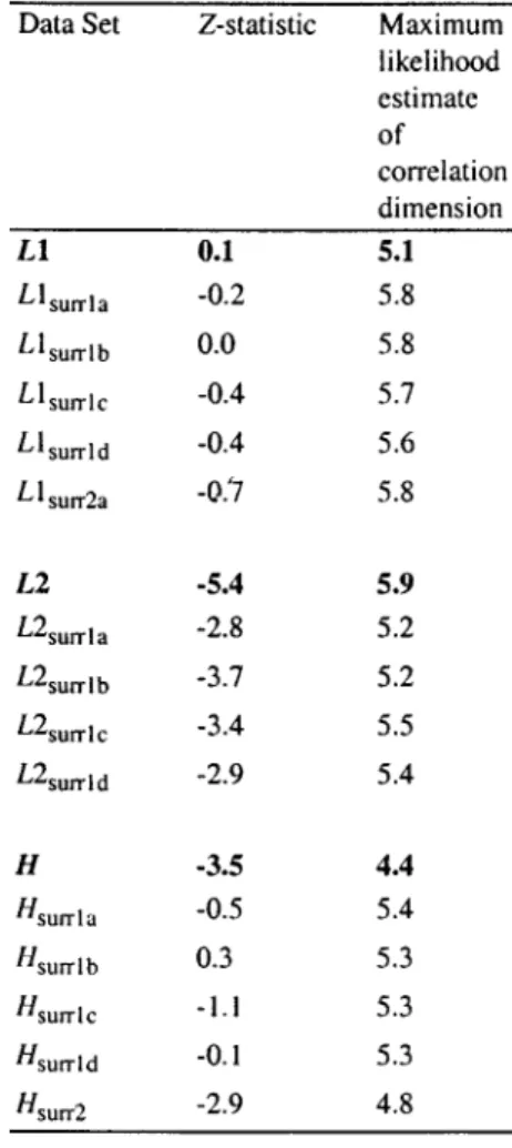
Table 1 summarizes the results of applying the test to the real-life and surrogate data sets. The calculations
involving surrogate data sets , and
were repeated four times with different random seeds to get a feel for the variability of the -statistic (and chaotic invariants to be discussed). Based on the results summarized in Table 1, we may state the following.
1) Sea clutter is nonlinear (i.e., is less than 3) when the sea state is high.
2) Sea clutter may be viewed as linear (i.e., is consider-ably larger than 3) when the sea state is low and the ocean waves are moving away from the radar. How-ever, when the ocean waves are coming toward the radar, sea clutter is nonlinear (i.e., is less than 3) even when the sea state is low.
3) The surrogate data sets have larger values (i.e., less evidence for nonlinearity) than their original
counter-parts. (Surrogate data sets and
are linear by construction.)
On the basis of these results, we may state that sea clutter is a nonlinear dynamical process, with the nonlinearity de-pending on the sea state being moderate or higher and the ocean waves moving toward or away from the radar.
The next question to be discussed is whether sea clutter is close to being deterministic chaotic. If so, we may then apply the powerful concepts of chaos theory.
B. Chaotic Invariants
In the context of a chaotic process, two principal features, namely, the correlation dimension and Lyapunov exponents, have emerged as invariants, with each one of them high-lighting a distinctive characteristic of the process.
Table 1
Summary ofZ Tests and Correlation Dimension
Physical processes that require an external source of energy are dissipative. For sea clutter, wind and temperature differences (caused by solar radiation) are the external sources of energy. A dissipative chaotic system is char-acterized by its own attractor. Consider then the set of all admissible initial conditions in the multidimensional state space of the system and call this the initial volume. The existence of an attractor implies that the initial volume eventually collapses onto a geometric region whose dimen-sionality is smaller than that of the original state space. Typically, the attractor has a multisheet structure that arises from the interplay between stabilizing and disrupting forces. The correlation dimension, originated by Grassberger and Procaccia [12], provides an invariant measure of the geom-etry of the attractor. For a chaotic process, the correlation dimension is always fractal (i.e., noninteger).
Whereas the correlation dimension characterizes the distribution of points in the state space of the attractor, the Lyapunov exponents describe the action of the dynamics defining the evolution of the attractor’s trajectories. Suppose that we now picture a small sphere of initial conditions around a point in the state space of the attractor and then allow each initial condition to evolve in accordance with the nonlinear dynamics of the attractor. Then, we find that in the course of time the small sphere of initial conditions
evolves into an ellipsoid. The Lyapunov exponents measure the exponential rate of growth or shrinkage of the principal axes of the evolving ellipsoid. For a process to be chaotic, at least one of the Lyapunov exponents must be positive so as to satisfy the requirement of sensitivity to initial conditions. Moreover, the sum of all Lyapunov exponents must be negative so as to satisfy the dissipative requirement.
With this brief overview of chaotic dynamics, we return to the subject at hand: the nonlinear dynamics of sea clutter.
In an article published in 1990, Leung and Haykin [19] posed the following question: “Is there a radar clutter at-tractor?” By applying the Grassberger–Procaccia algorithm to sea clutter, Leung and Haykin obtained a fractal dimension between six and nine. Independently of this work, Palmer et al. [20] obtained a value between five and eight for the cor-relation dimension of sea clutter.
These initial findings prompted Haykin and coinvestiga-tors to probe more deeply into the possible characterization of sea clutter as a chaotic process by looking into the second invariant: Lyapunov exponents. Haykin and Li [22] reported one positive Lyapunov exponent followed by an exponent very close to zero and several negative exponents. This was followed by a more detailed investigation by Haykin and Puthusserypady [23], using state-of-the-art algorithms:
1) a maximum-likelihood-based algorithm for estimating the correlation dimension [56];
2) an algorithm based on Shannon’s mutual information for measuring the embedding delay [57], [58]; 3) global embedding dimension, using the method of
false nearest neighbors [59]; the embedding dimen-sion is defined as the smallest integer dimendimen-sion that unfolds the attractor;
4) local embedding dimension, using the method of local false nearest neighbors [60]; the local embedding di-mension specifies the size of the Lyapunov spectrum; 5) an algorithm for estimating the Lyapunov exponents, which involves recursive QR decomposition applied to the Jacobian of a function that maps points on the trajectory of the attractor into corresponding points a prescribed number of time steps later [61], [62]. The findings reported by Haykin and Puthusserypady [23] are summarized as follows:
1) correlation dimension between four and five;
2) Lyapunov spectrum consisting essentially of five ex-ponents, with two positive, one close to zero, and the remaining ones negative, with the sum of all the expo-nents being negative;
3) Kaplan–Yorke dimension, derived from the Lyapunov spectrum, very close to the correlation dimension. These findings were so compelling, in light of known chaos theory, that the generation of sea clutter was concluded to be the result of a chaotic mechanism, on which we have more to say in Section III-E.
C. Inconclusive Experimental Results on the Chaotic Invariants of Sea Clutter
The algorithms currently available for estimating the chaotic invariants of experimental time series work very
Table 2
Summary of Lyapunov Exponents
well indeed when the data are produced by mathematically derived chaotic models (e.g., the Lorenz attractor), even in the presence of additive white noise so long as the SNR is moderately high. Unfortunately, they do not have the necessary discriminative power to distinguish between a deterministic chaotic process and a stochastic process. We have found this serious limitation for all the algorithms in our chaos analysis toolbox. The estimates of the correlation dimension and Lyapunov spectrum are summarized in Tables 1 and 2. Based on these results, we may make the following observations.
1) Examining the last column of Table 1 on the max-imum-likelihood estimate of the correlation dimen-sion, we see that for all practical purposes, there is little difference between the correlation dimension of sea-clutter data and that of their surrogate counterparts that are known to be stochastic by design.
2) Examining Table 2 on the estimates of Lyapunov spectra and the derived Kaplan–Yorke dimension, we again see that a test based on Lyapunov exponents is incapable of distinguishing between the dynamics of sea-clutter data and their respective stochastic surro-gates. Similar results on the inadequate discriminative power of these algorithms are reported in [63]. We, thus, conclude that although sea clutter is nonlinear, its chaotic invariants are essentially the same as those of the surrogates that are known to be stochastic. The notion of
non-linearity alone does not imply deterministic chaos; it merely excludes the possibility that a linear mechanism is respon-sible for the generation of sea clutter.
D. Dynamic Reconstruction
All along, the driving force for the work done by Haykin and coinvestigators has been the formulation of a robust dy-namic reconstruction algorithm to make physical sense of real-life sea clutter by capturing its underlying dynamics. Such an algorithm is essential for the reliable modeling of sea clutter and the improved detection of a target in sea clutter. Successful development of such a dynamical reconstruction algorithm was also considered to be further evidence of de-terministic chaos as the descriptor of sea-clutter dynamics.
To describe the dynamic reconstruction problem, with chaos theory in mind, consider an attractor whose process equation is noiseless, and whose measurement noise is additive, as shown by the following:
(9) (10) Suppose that we use the set of noisy observations
to construct the vector
(11) where is the embedding delay equal to an integer number of time units and is the embedding dimension. As the obser-vations evolve in time, the vector defines the underlying attractor, thereby providing a fiducial trajectory. The stage is now set for stating the delay-embedding theorem due to [10], [11], and [16].
Given the experimental time series of a single scalar component of a nonlinear dynamical system, the geometric structure of the hidden dynamics of that system can be unfolded in a topologically equivalent manner in
that the evolution of the points in the
reconstructed state space follows the evolution of the points in the original state space, provided that , where is the fractal dimension of the system and the vector is related to the given time series
by (11).
Ideas leading to the formulation of the delay-embedding theorem were described in an earlier paper by Packard et al. [9].
A key point to note here is that since all the variables of the system are geometrically related to each other in a non-linear manner, as shown in (9) and (10), measurements made on a single component of the nonlinear dynamical system contain sufficient information to reconstruct the multidimen-sional state .
Derivation of the delay-embedding theorem rests on two key assumptions:
1) the model is noiseless, i.e., not only is the state equa-tion (9) noiseless, but the measurement equaequa-tion (10) is also noiseless [i.e., ];
2) the observable data set is infinitely long.
Under these conditions, the theorem works with any delay so long as the embedding dimension is large enough to unfold the underlying dynamics of the process of interest.
Nevertheless, given the reality of a noisy dynamical model described by (9) and (10) and given a finite record of
obser-vations , the delay-embedding theorem may be
applied provided that a “reliable” method is used for esti-mating the embedding delay . According to Abarbanel [64], the recommended method is to compute that particular for which the mutual information between and its de-layed version attains its minimum value and the recommended method for estimating the embedding dimen-sions is to use the method of false nearest neighbors.
A distinction must be made between dynamic recon-struction and predictive modeling. Predictive modeling is an open-loop operation, which merely requires that the prediction error (i.e., the difference between the present value of a time series and its nonlinear prediction based on a prescribed set of past values of the time series) be minimized in the mean-square sense. Dynamic reconstruction is more profound in that it builds on a predictive model by requiring closed-loop operation. Specifically, the predictive model is initialized with data drawn from the same process under study, but not seen before and then the model’s output is delayed by one time unit and fed back to the input layer of the model, making room for this new input sample by leaving out the oldest sample in the initializing data set. This procedure is continued until the entire initializing data set is completely disposed of. Thereafter, the model operates in an autonomous manner, producing an output time series learned from the data during the training (i.e., open-loop predictive) session.
It is amazing that dynamic reconstruction, as described herein, works well for time series derived from mathemat-ical models of deterministic chaos, even when the time se-ries is purposely contaminated with additive white noise of relatively moderate average power (see, e.g., [65]).
Unfortunately, despite the persistent use of different reconstruction procedures involving the use of a multilayer perceptron trained with the back-propagation algorithm [22], regularized radial-basis function networks [66], and recurrent multilayer perceptrons trained with the extended Kalman filter [65], the formulation of a reliable procedure for the dynamic reconstruction of sea clutter based on the delay-embedding theorem has eluded us. The key question is: why? A feasible answer is offered in Section III-E.
Serious difficulties with the dynamic reconstruction of sea clutter prompted the authors of this paper in September 2000 to question the validity of a chaotic model for describing the nonlinear dynamics of sea clutter, despite the highly en-couraging results summarized in Section III. Indeed, it was because of these serious concerns that a complete reexam-ination of the nonlinear dynamical modeling of sea clutter was undertaken, as detailed in Section IV. However, before moving onto that section, we conclude the present discus-sion on chaos by highlighting some important lessons learned from our work on the application of deterministic chaos to sea clutter.
E. Chaos, a Self-Fulfilling Prophecy?
Chaos theory provides the mathematical basis of an ele-gant discipline for explaining complex physical phenomena using relatively simple nonlinear dynamical models. As with every scientific discipline that requires experimentation with real-life data, we clearly need reliable algorithms for esti-mating the basic parameters that characterize the physical phenomenon of interest, given an experimental time series. As already mentioned, there are two invariants that are basic to the characterization of a chaotic process:
1) correlation dimension; 2) Lyapunov exponents.
Unfortunately, state-of-the-art algorithms for estimating these invariants do not have the necessary discriminative power to distinguish between a deterministic chaotic process and a stochastic process. For the experimenter who hopes his/her data qualify for a deterministic chaotic model, the results of a chaotic invariant analysis may end up working as a self-fulfilling prophecy, indicating the existence of deterministic chaos regardless of whether the data are really chaotic or not. The stochastic process could be colored noise or a nonlinear dynamical process whose state-space model includes dynamical noise in the process equation. As pointed out in Sugihara [67], when we have noise in both the process and measurement equations of a nonlinear dynamical model, there is unavoidable practical difficulty in disentangling the dynamical (process) noise from the measurement noise to reconstruct an invariant measure. Specifically, in the estimation of Lyapunov exponents, it is no longer possible to compute meaningful products of Jacobians from the experimental time series because the invariant measure is contaminated with noise.
How do we explain the possible presence of dynamical noise in the state-space model of sea clutter? To answer this question, we first need to remind ourselves that ocean dy-namics are affected by a variety of forces, as summarized here [50]:
1) gravitational and rotational forces, which permeate the entire fluid, with large scales compared with most other forces;
2) thermodynamic forces, such as radiative transfer, heating, cooling, precipitation, and evaporation; 3) mechanical forces, such as surface wind stress,
atmo-spheric pressure variations, and other mechanical per-turbations;
4) internal forces—pressure and viscosity—exerted by one portion of the fluid on other parts.
With all these forces acting on the ocean dynamics and, there-fore, directly or indirectly influencing radar backscatter from the ocean surface, three effects arise:
1) evolution of the hidden state characterizing the under-lying dynamics of sea clutter due to the constant state of motion of the ocean surface;
2) generation of some form of dynamical noise, contam-inating this evolution with time, due to the natural rate of variability of the forces acting on the ocean surface;
3) imposition of a nonstationary spatio-temporal struc-ture on the radar observable(s).
Hence, given the physical reality that in addition to measure-ment noise, there is dynamical noise to deal with and the fact that there is usually no prior knowledge of the measurement noise or dynamical noise, it is not surprising that the dynamic reconstruction of sea clutter using experimental time series is a very difficult proposition.
IV. HYBRIDAM/FM MODEL OFSEACLUTTER
In Section III, we have expressed doubts on the validity of the deterministic chaos approach as the descriptor of sea clutter. In this section, we take a detailed look at several ex-perimental data sets to explore new ways to model sea clutter. Apart from the classical approaches reviewed in Section II, one source of inspiration is the recent work of Gini and Greco [68], who view sea clutter as a fast “speckle” process, mul-tiplied by a “texture” component that represents the slowly varying mean power level of the data—caused by large waves passing though the observed ocean patch. They model the speckle as a stationary compound complex Gaussian process and the texture as a harmonic process. What we will find is that the relationship between the slow and fast varying process is much more involved than what has been assumed so far in the literature. In particular, we find that the slowly varying component does not only modulate the amplitude of the speckle, but also its mean frequency and spectral width. A. Radar Return Plots
We use the data sets and from Appendix B. The analysis starts by looking at the radar return plots of these data sets, shown in Fig. 5. These plots show the strength of the radar return signal (color axis) as a function of time ( axis) and range ( axis). A red color indicates a strong return, which is associated with wave crests. The diagonal red stripes in both plots show that the wave crests move, with increasing time, toward a decreasing range or toward the radar. Indeed we see from Appendix B that the wind and radar beam point in almost opposite directions. If we look at a single range bin, i.e., along a horizontal line in the radar return plots, we see that the strength of the return signal is roughly periodic, with a period in the order of 4–8 s, corre-sponding to the period of the gravity waves (see Section II). In Fig. 1(a)–(c), such a single range bin is plotted against time, the axis now being return strength (amplitude of the received signal). The periodic behavior is less pronounced due to the wild short-term fluctuations of the signal, which are caused by Rayleigh fading.
B. Rayleigh Fading
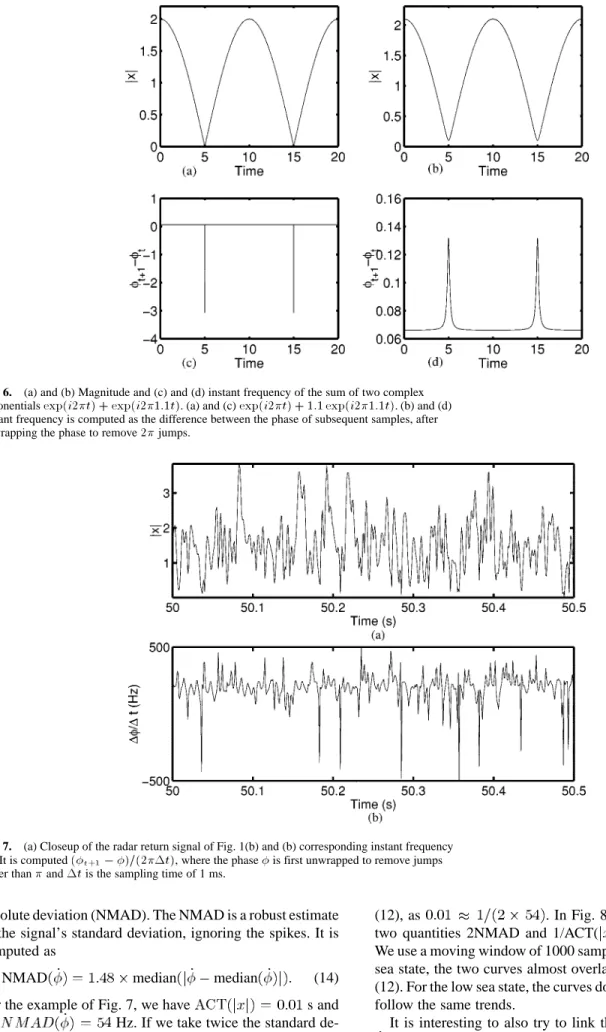
Rayleigh fading arises when a number of complex expo-nentials of slightly different frequency are added together. Fig. 6 shows the magnitude and instantaneous frequency of
the sum , with
, and is varied and denotes the square root of 1. In Fig. 6(a), is equal to and in
Fig. 5. Radar return versus time and range, VV polarization, of (a) data setL2 (low sea state) and (b) data setH (high sea state). Color axis shows log(j~xj), where ~x is the complex envelope of the unreceived signal. Units~x are normalized and the color axis changes from blue (low) via green to red (high).
Fig. 6(b), it is 10% larger. The figure illustrates the typical upside down U shape of the magnitude of a Rayleigh fading process, with a period that follows
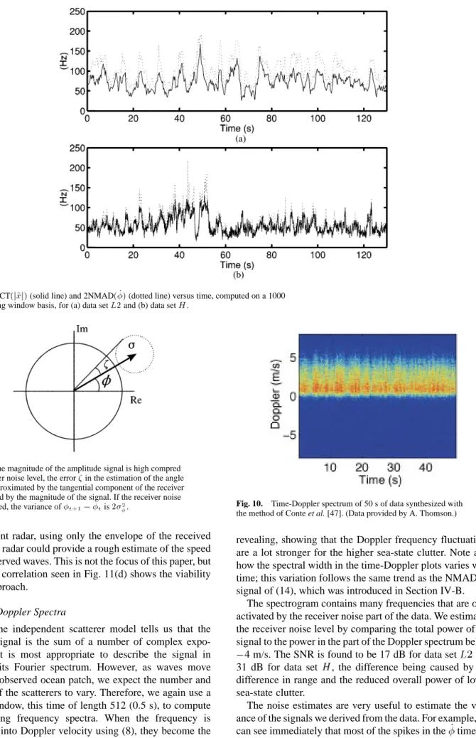
(12) Looking at the closeup of our data in Fig. 7, we see that both the magnitude and instantaneous frequency have the typical characteristics of Rayleigh fading, although in Section IV-C, we will find that most spikes in the time series are actually caused by receiver noise.
Why does Rayleigh fading occur? The answer lies in the independent scatterer model that Jakeman and Pusey [27] first used to derive a physical justification for the use of the distribution (see Section II). If we think of a patch of ocean illuminated by the radar at a given time, according to this model, the received signal will be dominated by a small number of independent scatterers, each moving at its own ve-locity. We make the additional restriction that, at least for the short duration of a single sample time, each scatterer has its own constant velocity with respect to the radar. The received signal can then be written as
(13)
where is the angular radio frequency of the radar (equal 9.39 GHz for the IPIX radar), is the number of indepen-dent scatterers, is proportional to the effective radar
cross-section of scatterer , and and are the Doppler
frequency and phase of scatterer at time , respectively. After removing the carrier wave by multiplying by , we see that (13) is indeed a sum of complex exponentials with slightly different frequencies, thereby resulting in Rayleigh fading. The frequencies are related to the physical speed of the scatterer by (8).
Now that we have established the Rayleigh fading char-acteristics of sea clutter amplitude data, we go back to (12), which relates, for the case of two complex exponentials, the period of the amplitude signal to the frequency difference of the two exponentials. Sea clutter has much more than two complex exponentials and they are constantly changing frequency, but as a coarse approximation, (12) may still be useful. As a rough estimate for the average of sea clutter, we use the average cycle time (ACT) of the data: sub-tract the median of the signal and take the average time be-tween two upward zero crossings. For the left-hand term of (12), we need to estimate , the frequency variability of sea clutter. This we estimate by taking the measured in-stantaneous frequency and computing its normalized median
Fig. 6. (a) and (b) Magnitude and (c) and (d) instant frequency of the sum of two complex exponentialsexp(i2t) + exp(i21:1t). (a) and (c) exp(i2t) + 1:1 exp(i21:1t). (b) and (d) Instant frequency is computed as the difference between the phase of subsequent samples, after unwrapping the phase to remove2 jumps.
Fig. 7. (a) Closeup of the radar return signal of Fig. 1(b) and (b) corresponding instant frequency
_ . It is computed ( 0 )=(21t), where the phase is first unwrapped to remove jumps
larger than and 1t is the sampling time of 1 ms.
absolute deviation (NMAD). The NMAD is a robust estimate of the signal’s standard deviation, ignoring the spikes. It is computed as
NMAD median median (14)
For the example of Fig. 7, we have s and
Hz. If we take twice the standard de-viation as our measure of variability, then the result satisfies
(12), as . In Fig. 8, we look at how the
two quantities 2NMAD and 1/ACT( ) evolve with time. We use a moving window of 1000 samples (1 s). For the high sea state, the two curves almost overlap, in agreement with (12). For the low sea state, the curves do not overlap, but they follow the same trends.
It is interesting to also try to link the variability of to itself. If we could do this, then even with an inexpensive
Fig. 8. 1/ACT(j~xj) (solid line) and 2NMAD( _) (dotted line) versus time, computed on a 1000 sample sliding window basis, for (a) data setL2 and (b) data set H.
Fig. 9. If the magnitude of the amplitude signal is high compred to the receiver noise level, the error in the estimation of the angle
can be approximated by the tangential component of the receiver
noise, divided by the magnitude of the signal. If the receiver noise is uncorrelated, the variance of 0 is 2 .
noncoherent radar, using only the envelope of the received signal, the radar could provide a rough estimate of the speed of the observed waves. This is not the focus of this paper, but the strong correlation seen in Fig. 11(d) shows the viability of this approach.
C. Time-Doppler Spectra
Since the independent scatterer model tells us that the received signal is the sum of a number of complex expo-nentials, it is most appropriate to describe the signal in terms of its Fourier spectrum. However, as waves move along the observed ocean patch, we expect the number and strength of the scatterers to vary. Therefore, we again use a sliding window, this time of length 512 (0.5 s), to compute time-varying frequency spectra. When the frequency is converted into Doppler velocity using (8), they become the time-Doppler spectra of Fig. 2(a)–(c). The plots are very
Fig. 10. Time-Doppler spectrum of 50 s of data synthesized with the method of Conte et al. [47]. (Data provided by A. Thomson.) revealing, showing that the Doppler frequency fluctuations are a lot stronger for the higher sea-state clutter. Note also how the spectral width in the time-Doppler plots varies with time; this variation follows the same trend as the NMAD( ) signal of (14), which was introduced in Section IV-B.
The spectrogram contains many frequencies that are only activated by the receiver noise part of the data. We estimated the receiver noise level by comparing the total power of the signal to the power in the part of the Doppler spectrum below 4 m/s. The SNR is found to be 17 dB for data set and 31 dB for data set , the difference being caused by the difference in range and the reduced overall power of lower sea-state clutter.
The noise estimates are very useful to estimate the vari-ance of the signals we derived from the data. For example, we can see immediately that most of the spikes in the time se-ries occur when the signal drops below the noise floor. What
Fig. 11. (a) and (c) Low-pass-filtered amplitude (1 s averaging). (b) and (d) Low-pass-filtered instant frequency _ (solid line) and NMAD ( _) (dotted line). (a) and (b) Data set L2. (c) and (d) Data set H. is the variance of the signal? If the magnitude of the signal
is well above the noise floor, can be estimated using (see Fig. 9)
where is the receiver noise level. From this estimate, it appears that the NMAD( ) signal in Fig. 8(a) (data set ) is dominated by receiver noise, whereas in Fig. 8(b) (data set ), it is dominated by the clutter signal. For data set , this means that we now expect an inverse relationship between NMAD( ) and the amplitude of the signal. This relationship is clearly visible if we compare the solid line in Fig. 11(a) to the dotted line in Fig. 11(b).
D. Amplitude Modulation, Frequency Modulation, and More
Almost invariably, models for sea clutter distinguish be-tween the slow time scale of the gravity waves and the fast time scale of the capillary waves. A typical approach is that of Conte et al. [43], consisting of a colored noise process that is amplitude-modulated by a slowly varying intensity com-ponent. Fig. 10 shows the time-Doppler spectrum for such data. The results in the previous sections teach us that there is a much more intricate relationship between the fast- and the slow-varying processes.
When a large wave passes through the ocean patch under surveillance, it will first accelerate and then decelerate the water on the ocean surface. The tilting of the ocean surface by the wave causes the amplitude modulation. Even if scatterers arise mostly on the crest of the wave, the wave will cause a cyclic motion of the velocity of the scatterers. This motion is widely recognized, but its consequence, namely, a frequency modulation of the speckle component, has been neglected. And there is more. When the mean velocity of the scatterers is high at a given instant, then the spread around that mean is also high. We can now explain why almost invariably we found sea clutter to be nonlinear, when we presented the re-sults in Table 1. Recognizing that amplitude modulation is a linear form of modulation, but frequency modulation is not [69], we expect the value of to become more negative as the amount of frequency modulation increases. Fig. 12 confirms this qualitative relationship by plotting the value versus the amount of frequency modulation. Apart from the datasets and , the figure uses an additional 75 datasets from our sea-clutter database, measured at a wide variety of experimental conditions. It is no surprise that the surrogate data sets used in Table 1 are less nonlinear than their orig-inal counterparts, since the random phase shifting partially destroys the frequency modulation. The typical “breathing” seen in time-Doppler plots, such as the ones in Fig. 2, shows that not only the mean of the velocity spectrum, but also its spectral width are modulated. Moreover, in some cases, the
Fig. 12. Z value versus NMAD ( _), computed for 78 datasets measured by the IPIX radar at various experimental conditions.
velocity spectrum even has a bimodal distribution [around time 45 to 50 s in Fig. 2(b)]; recent work of Walker [48] shows that this is most likely caused by a breaking wave.
So far, we have identified four different processes acting on the dynamics of the speckle component: 1) amplitude modulation; 2) frequency modulation; 3) spectral-width modulation; and 4) bimodal frequency distributions due to breaking waves. All these processes, which have the slow time scale of gravity waves, need to be specified in order to synthesize artificial radar data. In Fig. 11, we look for possible correlation between the various types of modula-tion. The relation between the amplitude modulation and frequency modulation seems weak [compare solid lines in Fig. 11(a) to (b) and (c) to (d)]. Fig. 11(d) shows that there is a strong correlation between the frequency modulation ( averaged over 1 s) and the spectral-width modulation, measured by NMAD( ). This correlation is not confirmed by the equivalent plots for low sea state in Fig. 11(b), but is due to receiver noise, as argued in Section IV-C.
E. Modeling Sea Clutter as a Nonstationary Complex Autoregressive Process
So far, our results have not made the sea-clutter synthesis much easier—it seems we almost have to provide the en-tire time-Doppler spectrum to get a complete signature of the observed data. As a first step toward a practical algo-rithm, in this section, we compress the time-Doppler spec-trum into only a few complex parameters per time slot and, at the same time, we make it suitable for time-series gener-ation. We argue as follows, using observations from the pre-ceding discussion.
1) On time-scales shorter than several seconds, sea clutter can be described as the sum of complex exponentials. 2) A sum of complex exponentials is well described in
terms of its Fourier spectrum.
3) The Fourier spectrum of a dynamical system can often be approximated most efficiently by an AR process.
This brings us to the concept of a time-varying complex AR process. We take a 1-s window (1000 samples), slide it through data set (pertaining to a higher sea state) with small time increments, and each time we fit a complex AR process to the data. We search for the lowest order time-varying AR model that approximates the short-time Fourier transforms (vertical lines in the time-Doppler spec-trum) well. When we increase the order from one to four, the standard deviation of the residual error, averaged over time, decreases: 0.23, 0.11, 0.091, 0.086 in units of signal standard deviations. In the same units, the receiver noise as estimated from the time-Doppler spectrum is 0.061. The improvement with model order is very clear from Fig. 13, which shows time-Doppler spectra of synthesized clutter, using time-varying AR processes of order one, two, and three, denoted as AR(1), AR(2), and AR(3), respectively. The data are generated according to the difference equation
(15) where all variables are complex, are the AR
coeffi-cients at time with , the brackets indicate
that they change on a slow time scale only, is the model order, and is the noise process having a time-varying
variance .
The AR model of order 1 is clearly insufficient to describe sea clutter in good detail, but it is by far the easiest to analyze in physical terms. It has three independent parameters that vary slowly with time: 1) the amplitude of ; 2) the angle of ; and 3) the variance of the noise . Fig. 14 shows how these three independent parameters are coupled to the three main types of modulation mentioned in Section IV-D. Indeed, we could rewrite the nonstationary AR(1) process into an equivalent stationary AR(1) process, modulated in amplitude, frequency, and spectral width. Unfortunately, the sliding AR(1) does not provide a good enough description of the data and we need to investigate in future work what phys-ical mechanism it is that the AR(2) and AR(3) have captured but the AR(1) has not.
V. DISCUSSION ANDCONCLUSION
Sea clutter, referring to radar backscatter from an ocean surface, is a nonstationary complex nonlinear dynamical process with a discernible structure that exhibits a multitude of continuous-wave modulation processes: 1) amplitude modulation; 2) frequency modulation; 3) spectral-width modulation; and 4) bimodal frequency distribution due to breaking waves. The modulations are slowly varying (in the order of seconds) functions of time. The amplitude modulation is clearly discernible in the sea-clutter wave-form, regardless of the sea state or whether the ocean waves are moving away from the radar or coming toward it. The frequency modulation and variations in spectral width and spectral shape become clearly observable when the nonlinear nature of sea clutter becomes pronounced. This happens when the sea state is higher or the ocean waves are coming toward the radar. These observations on the nonlinearly
Fig. 13. Time-Doppler spectra of data synthesized by a sliding AR process of order (a) 1, (b) 2, and (c) 3. Three plots have identical color axis limits. Lighter background color in (a) is caused by the larger residual error of the sliding AR(1) model.
modulated nature of sea clutter have become clear from the detailed experimental study reported in Section IV. This study paves the way for a new phemenological approach to the modeling of sea clutter in terms of all its modulating components. In subsequent work, we will extend the work to the full body of experimental data that we gathered on the east coast of Nova Scotia in 1993. We have already developed a website that will also enable others to use this valuable resource and contribute to this exciting field.2
A. State-Space Theory
The adoption of a state-space model for sea clutter is a natural choice for describing the nonstationary nonlinear
dy-2See http://soma.crl.mcmaster.ca/ipix.
namics responsible for its generation. Most importantly, time features explicitly in such a description.
The challenge in the application of a state-space model to sea clutter is basically two-fold:
1) the formulation of the process and measurement equa-tions (including the respective dynamical and mea-surement noise processes), which are most appropriate for the physical realities of sea clutter;
2) the use of a computational procedure, which is not only efficient but also most revealing in terms of the phe-nomenological aspects of sea clutter.
Each of these two issues is important in its own way. In light of the material presented in Sections III and IV and contrary to conclusions reported in earlier papers [19]–[23], we have now come to the conclusion that sea clutter is not
Fig. 14. Amplitude, frequency, and spectral width modulation exhibited by the nonstationary complex AR(1) process, trained on a 1000-sample sliding window of data setH. (a)
Low-pass-filtered amplitude of data setH and of the model ( )=(1 0 ja j )(=2) versus time (plots overlap almost completely). (b) 1 s median-filtered ( _) and a f =(2) versus time. f is the pulse repetition frequency of 1000 Hz (plots overlap almost completely). (c) NMAD( _) (dotted line) and spectral width of the model, computed bycos ((1 0 4ja j + ja j )=(02ja j)) (see [77]) versus time.
the result of deterministic chaos.3 By definition, the process
equation of a deterministic chaotic process is noise-free. In reality, however, the process equation of sea clutter contains dynamical noise due to the fast fluctuations of the various forces, which act on the ocean surface. As pointed out by Heald and Stark [72], there is no physical system that is en-tirely free of noise and no mathematical model that is an exact representation of reality.4We must, therefore, expect noise in
both the process and measurement equations of sea clutter, with two important consequences.
1) There is unavoidable practical difficulty in disentan-gling the dynamical noise from the measurement noise when we try to reconstruct an invariant measure [67]. This may be the reason for why currently available algorithms for estimating chaotic invariants are
inca-3We do not rule out the possibility of stochastic chaos or a mixture of
sev-eral deterministic chaos as well as stochastic mechanisms being responsible for generating the nonlinear dynamics of sea clutter. The notion of stochastic chaos and related issues are discussed in [67], [70], and [71]. However, we do not have the tools to distinguish between stochastic chaos and stochastic processes using real-life data.
4Heald and Stark [72] describe a Bayesian procedure for estimating the
variance of dynamical noise for the case when the noise processes in the nonlinear state-space model are additive.
pable of discriminating between sea clutter and its sto-chastic surrogates.
2) The delay-embedding theorem for dynamic recon-struction is formulated on the premise of a deter-ministic process. Although, from an experimental perspective, it is possible to account for the presence of measurement noise through a proper choice of embedding delay and embedding dimension [64], it is difficult to get around the unavoidable presence of dynamical noise in the process equation. This may explain the reason why it is very difficult to build a predictive model for sea clutter that solves the dynamic reconstruction problem in a reliable manner. Next, addressing the issue of a computational procedure for studying the nonlinear dynamics of sea clutter, the use of a time-varying complex-valued AR model, as described in Section IV, is attractive for several reasons.
1) An AR model of relatively low order (four or five) appears to have the capability of capturing the major features of the nonlinear dynamics of sea clutter. 2) The AR model lends itself to a “phenomenological”