V
Š
B
–
TECHNICAL UNIVERSITY OF OSTRAVA
FACULTY OF ECONOMICS
DEPARTMENT OF FINANCE
Modelování e
fektů
p
řelévání
volatility
Modelling Volatility Spillover Effects
Student: Bc. Lingling Ding
Supervisor of the bachelor thesis: Ing. Petr Seda, Ph.D.
CONTENTS
1 INTRODUCTION…...………3
2 FINANCIAL MARKETS AND PROPERTIES OF FINANCIAL TIME SERIES………...5
2.1 Basic Characteristics of Financial Markets………5
2.1.1 Fundamental Information on Financial Markets………6
2.1.1.1 Basic Element to Form and Develop a Financial Market………6
2.1.1.2 Functions of the Financial Markets………6
2.1.2 The Classifications of Financial Markets………7
2.1.3 Importance of Financial Markets for Economics………8
2.2 Crises in Stock Markets………9
2.2.1 The Stock Market Crash of 1987……….9
2.2.2 The Dot-com Bubble………11
2.2.3 Global Financial Crisis of 2007-2009………12
2.3 Characteristics of Financial Time Series………13
2.3.1 Volatility Clustering………14
2.3.2 Leptokurtic Distribution………14
2.3.3 Leverage Effect………15
3 METHODOLOGY………18
3.1 Volatility Spillover Effect and its Importance………18
3.2 Literature Review………20
3.3 Univariate Volatility Models………21
3.3.1 ARCH Model………21
3.3.2 GARCH Model………22
3.3.3 The GARCH(1,1) Model………23
3.3.4 EGARCH Model………24
3.4 Price Spillover Models………25
3.4.1 The Stationarity of VAR Model………26
3.4.2 Advantages and Disadvantages of VAR Model………27
3.5 Volatility Spillover Models………27
4 DATA SAMPLE DESCRIPTION ………30
4.1 Characteristics of Investigated Stock Markets………30
4.1.1 French Stock Market………30
4.1.2 German Stock Market………31
4.1.4 Swiss Stock Market………32
4.2 Description of Investigated Indexes………32
4.2.1 Paris Stock Index CAC 40………33
4.2.2 Frankfurt Stock Index DAX 30………34
4.2.3 London Stock Index FTSE 100………36
4.2.4 Zurich Stock Index SMI 20………38
4.2.5 Eurozone Index EURO STOXX 50………40
4.2.6 US Index S&P 500………..41
4.3 Descriptive Statistics of Used Time Series………43
4.3.1 Returns in Financial Modeling………43
4.3.2 Definition of Testing Sub Periods………44
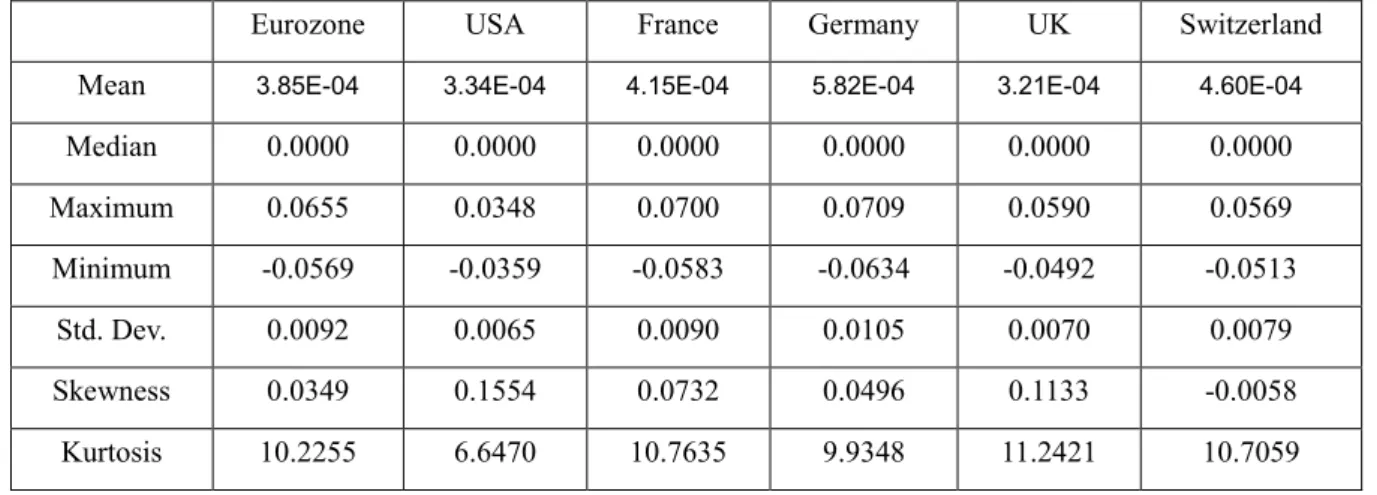
4.3.3 Descriptive Statistics in the Pre-Crisis Period………45
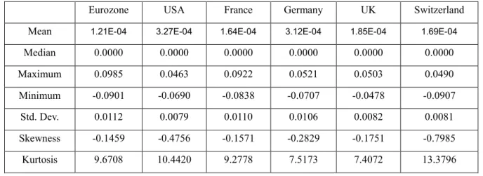
4.3.4 Descriptive Statistics in Crisis Period………46
4.3.5 Descriptive Statistics in the Post-Crisis Period………47
5 EMPIRICAL FINDINGS………48
5.1 Estimation of Univariate Volatility Models using EGARCH Model………48
5.1.1 Pre-Crisis Period………48
5.1.2 Crisis Period………50
5.1.3 Post-Crisis Period………52
5.2 Estimation of Price Volatility Spillover Models………54
5.2.1 Pre-Crisis Period………54
5.2.2 Crisis Period……….56
5.2.3 Post-Crisis Period………57
5.3 Estimation of AR/EGARCH Volatility Spillover Models………59
5.3.1 Pre-Crisis Period………59 5.3.2 Crisis Period………62 5.3.3 Post-Crisis Period………64 5.5 Summary of Results………66 6 CONCLUSION………69 BIBLIOGRAPHY………71 LIST OF ABBREVIATIONS………74 DECLARATION OF UTILISATION OF RESULTS FROM THE DIPLOMA THESIS LIST OF ANNEXES
1 Introduction
In contemporary society, almost all transactions in financial markets are recorded, which lead to a vast amount of data available on internet or other approaches. Therefore, a great deal of analysis and a host of predictions are existing in financial markets. The financial time series is one of the most significant tools for analysis and predictions. financial time series, hence, is playing a significant role in quantitative analysis in financial market. Besides, the volatility is an essential element for financial time series, which is considered when making decision. Moreover, there are different measures to estimate the volatility with the different financial situation.
It is generally arguable that the stock market is a critical segment of financial market to represent the current situation of finance. Hence, exploring the regularity of the stock market is consistently popular in this day and age. the fundamental and technical methods are the basic methods for analyzing the stock markets. Except that, the financial time series is using to exhibit the volatility of the indexes during a specialized period of time to analyze and predict the tendency of the stocks.
The main goal of this thesis is to investigate, compute and interpret volatility spillover effect in selected European developed stock markets using extended autoregressive conditional volatility models. In particular, there will be modelled an impact of volatility coming from US and Eurozone stock markets. For the purpose of this thesis, we utilize daily returns of US, Eurozone, German, French, British and Swiss stock markets covering the period from January 2003 to August 2017. All the stock markets will be approximated by main stock indexes.
The main goal of this thesis is supported by two sub-goals: the first sub-goal is to model and measure also the price spillover effect using VAR models; the second sub-goal is to investigate an impact of global financial crisis on volatility spillover effects.
Including the introduction and conclusion, the whole thesis is divided by six chapters. The financial market and financial time series are the fundamental knowledge of this thesis, therefore, in the chapter 2, it will start with a brief account of the basic information of financial markets. Then, the financial crises – the stock market crash of 1987, the dot-com bubble and the global financial crisis of 2007-2009 - in stock market will be described which would influent the trend of stock indexes. Moreover, the basic features of financial time series – volatility clustering, leptokurtic distribution and leverage effect – will be indicated.
For chapter 3, cause the price and volatility spillover effects are the essential results of the volatility, the methodologies to estimate them will be described in this chapter. Therefore, the VAR model will be introduced from basic interpretation, stationarity, and pros and cons. Besides, the four main sorts of the ARCH models – ARCH model, GARCH model, EGARCH model and AR/GARCH model – will be illustrated.
For chapter 4, firstly, the basic characteristics of investigated stock markets will be illustrated, and the most important stock indexes in investigated stock markets will also be introduced, in which the values and return of indexes will be analyzed. Moreover, the reasons and descriptive statistics of used time series will be explained and analyzed.
For chapter 5, according to the chapter 3, firstly, the non-linear models – EGARCH (1,1) models - will be established as well as the conditional variances will be analyzed in each stock markets in each period. Furthermore, the VAR models will estimate the price spillover effects for investigated stock market in given periods. Moreover, AR/EGARCH models will estimate and test the price and volatility spillover effects and variance ratios will be computed. Lastly, comparing the results of models above, getting the summary of estimation.
For chapter 6, it will summarize the whole thesis, evaluating if the purpose of this thesis is fulfilled.
Taking a panoramic view of the thesis, the figures in the chapter 2 and 3 are mainly from the reference of the books, while the figures and tables in the chapter 4 and 5 are from the statistical software Eviews 7.2.
2 Financial Markets and Financial Time Series
In this chapter, the basic characteristics of financial markets and financial time series will be descripted. In the first place, there is a brief description of the fundamental information on financial markets, and why the financial market is important in the economy will be indicated. Furthermore, the three stock crises, which influenced the European financial markets, will be described. More importantly, the last subchapter will illustrate volatility clustering, leptokurtic distribution and leverage effect which are the basic features of financial time series. There are a vast number of textbooks available. The basic concepts of financial markets can be got from Mishkin (2004) and Jurgen, F. and Christian, M. (2012), moreover explanations of financial time series will be introduced briefly by Campbell, Lo and MacKinlay (1997), Mandelbrot (1963).
2.1 Basic Characteristics of Financial Markets
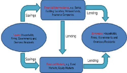
Financial markets are markets, in which funds are transferred from people who have extra funds to people who want more funds to invest. “Without financial markets and the institutional structure that supports them, selling the assets we own would be extremely difficult.” (Cecchetti and Schoenholtz, 2015).
Figure 2.1 Flows of funds through the financial system
Source: Mishkin, F. (2004)
economies while it is the fundamental purpose of financial markets, transferring the funds. Hence, this subchapter will describe the basic information of financial markets.
2.1.1 Fundamental Information on Financial Markets
A financial market is a market where the financial instruments are traded and exchanged. As a financial market, there are two basic elements which are essential.
2.1.1.1
Basic Element to Form and Develop a Financial Market
a) First of all, the suppliers of funds and demanders of funds are requisite, including government, financial instruments, residents, foreign businesses and so on. The suppliers provide extra funds and the demanders raise funds from financial markets, both are indispensable. It is the basic element to form and develop a financial market.
b) Moreover, financial instruments are also important. A financial instrument is a monetary contract between two parties, writing a legal obligation of one party to transfer something of value to another party at a certain future date. Bonds, stocks, bills, insurance are examples of financial instruments.
c) Lastly, it is about financial intermediaries. A financial intermediary is an institution or individual between who wants to purchase financial instruments and who wants to issue them. Banks, investment companies, insurance companies, brokers are all financial intermediaries.
2.1.1.2
Functions of the Financial Markets
With a financial market, a further comprehension is necessary – functions of the financial markets. There are three main functions served as financial markets, which include market liquidity, information and risk sharing.
Financial markets offer the market liquidity to lenders and borrowers, to ensure the lenders or borrowers can sell or buy the instruments easily and cheaply. If a market has so many buyers and sellers, it can be said that the market has high market liquidity. Normally, the traders are willing to invest in liquidity financial instruments, such as stock, bond and so on, to instead of investing in non-current financial instruments, such as real estate.
Moreover, Financial markets pool and communicate information about the financial instruments. In financial markets lenders and borrowers are easier to get a mass of information with low costs, comparing with the information which they got, they can invest some financial
instruments with low risk and high return, and they even allow have a portfolio with their funds. Furthermore, Financial markets are the place where you can transfer risk. Investors can buy or sell risks while sharing them with others in financial markets. Investors would allow holding ones if they think is low risk, and they also can get rid of ones if it is high risk. And investors can choose different financial instruments together as a portfolio to reduce risk. Anyway, it just can be in financial markets that sharing risk.
2.1.2
The Classifications of Financial Markets
In the world, there are a lot of financial markets, hence, it is necessary to categorize them with different ways to make people get it easier.
a) Firstly, we can categorize the markets by maturity of claim – Money market and capital market. Money market is a market where financial instruments are traded with high liquidity and very short maturities. Lenders and borrowers can sell or buy in the short term with maturities up to one year. The financial instruments in money market have small yield. And the main money markets securities are treasury-bills, commercial papers, negotiable certificates of deposit and so on. Capital market is a market where buys and sells equity and debt instruments. It is the market for long-term loans and equity capital. In this market, the maturity of it is more than one year, hence, it has lower liquidity compared with money markets. Furthermore, the financial instruments in capital market have various risk.
b) Secondly, we can distinguish between debt market and equity market which classification by nature of claim. Debt market also can be called bond market, it means that bonds are issued and traded in this market. Bondholders will have a fixed payment, usually with interest, and bonds have maturity date. Equity can be named as stock market, it is a market where stocks are issued and traded. The return to stockholders are less assured because the dividends can be easy changed. Moreover, stocks do not have maturity date while the stockholder is one of the owners of the business.
c) Thirdly, we can group them based on the type of seasoning – primary market and secondary market. The primary market is a market which issues new securities on a stock exchange for business to obtain financing. After financial instruments are issued in the primary market, they are trading in the secondary market. The secondary market offers issues information and liquidity.
For the purpose of this thesis, the equity market, classified by nature of claim, will be used as the background information.
2.1.3 Importance of Financial Markets for Economics
In the present age, business firms need large amounts of capital to finance their operations. In the financial market, they can raise funds from investors by selling stock or bonds. Additionally, the government also needs funds to provide goods and services. With the financial markets, government can borrow funds by selling bonds. Whatever bonds, stocks or other financial instruments, which used in our life, is trading in financial markets, hence, the financial markets are essential. Totally, this subchapter will discuss why the financial markets are important for economics clearly.
Firstly, the readers need comprehend the main subjects of the financial market, which include banks, investment banking firms, savings and loan associations, pension funds, insurance companies etc. Hence, some main subjects will be described.
Starting from commercial banks, they provide banking and other financial services and they represent the most important financial intermediary. As a bank, the banking license is necessary, which are granted by financial supervision authorities and provide rights to conduct the most fundamental banking services, the most common services are accepting deposits and making loans. Furthermore, pension fund is setting up by a corporation, labor union, governmental entity or other organization to pay the pension benefits of retired workers. Lastly, insurance companies are the business of providing protection against financial aspects of risk. Those financial instruments are everywhere in this day and age; therefore, financial markets are important to economics.
Moreover, this subchapter will show the benefit of the financial markets for economics. a) Possibility of obtaining funds. The units who are deficit can obtain funds in the financial markets, and it means they can borrow the money in the financial markets and not only from banks;
b)Motivation factor. As a rational investor, low risk and high return are best. And the financial markets satisfy what investors want. Hence, it can motivate investors to invest their money through financial markets;
c) Information of price. Periodic trading of a security reveals the consentaneous price which an assets commands on the market. Hence, if an issuer wants to invest new securities, the investor would know what the price level must be set for new bonds or stocks;
d)Liquidity in financial markets. Liquidity provides investors an opportunity to reverse the trade. It means that investors can sell or purchase securities if they want;
and sellers to trade, which place is called secondary markets, and it will reduce search costs because of the brokers and dealers. Transaction costs would be kept low with large trading quantities and continuous trading;
f) Reduce risk. Investors can invest a lot of different financial instruments simultaneously, they can make the portfolios what they want.
All of them would promote the development of economics and improve the importance of economics in the world. Therefore, financial markets are important to economics.
2.2 Crises in Stock Markets
Stock market is one of the biggest financial markets in the contemporary world economy. Thus, the development process of the stock market could influence the developing direction of the financial markets. Moreover, the development process of the stock market could not be always successful, it always moves in zigzags and by roundabout ways. That is why there have crises in stock markets, and it is characterized as huge fluctuation of financial assets in the secondary market, such as the market prices of stock markets, bond markets, fund markets and derivatives markets change to depreciate rapidly.
This subchapter will indicate three typical crises in stock markets, which have deepest influence on Euro area, to comprehend, including the Stock Market Crash of 1987, the Dot-com Bubble from 1997 to 2001 and the global financial crisis of 2007.
Before talking that, there is a briefly account of types of financial crises. There have three categories of financial crises – banking crises, currency crises, and sovereign debt crises.
It is a banking crisis if the significant signs of financial distress were in the banking system, and if the significant banking policy intervention measures in response to significant losses in the banking system; if it was a currency crisis, the currency would be in depreciation; a sovereign debt crisis is when a country is unable to pay its bills.
2.2.1 The Stock Market Crash of 1987
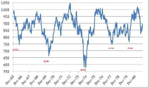
After the WWII, with the greatly enhanced of the economic strength of the United States, all kinds of investment activities were very active, and the stock market turned into a prosperous stage. The index of stock was a very substantial increase in the 1950s, and there was a peak in 1966, and the Dow Jones Industrial Average (DJIA) Index was closed to 1000 points (Figure 2,2). As showing in the Figure 2.2, during the 1966 to 1981, the price of stock had been in a state of volatility. In the early 1980s, the price of stock started to rise, reaching
to 1036 points on October 21, 1982, which broken the highest point in past ten years. In the same year, the DJIA raised to 1065 on November 3, which was the highest points after the WWII. Since then, the DJIA was increasing in the next five years. The DJIA reached to 1896 points, increasing by 78% compared with 1982. In the start of the 1987, the price of stock raised rapidly, and the DJIA reached to 2722 on August.
Figure 2.2 The Dow Jones Industrial Average from 1966 to 1981
Source: by author
However, looking at the Figure 2.3, on Monday, October 19, 1987, a wave of stock plummeting started from the New York stock market on Wall Street, triggering the largest crash in the history. The DJIA tumbled 508.32 points in that day, dropping 22.6%, the highest one-day decline since 1941. Within 6.5 hours, the stock market in the New York lost 500 billion U.S. dollars, which equivalent to one-eighth of the annual GDP of the United States. The plunge in the New York stock market shocked the entire financial market, and it created a domino effect in the stock markets around world, especially, the stock markets in the London, Frankfurt, Tokyo, Sydney, Hong Kong, and Singapore were suffered very strong shock, the shares declining more than 10%.
The plummeting stock market caused a great panic among the shareholders, many millionaires became the poor overnight nervous breakdowns. This day was called “the Black Monday” in the financial market, and the New York Times said it was “Well Street’s blackest hours”.
Figure 2.3 The Dow Jones Industrial Average from 1982 to 1997
Source: by author
2.2.2 The Dot-Com Bubble
In the 1990s, the U.S. economy recovered and was growing around 110 months with the rapid economic growth, low inflation, low unemployment and low deficits working together.
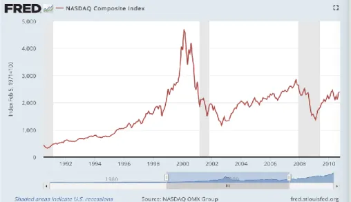
Figure 2.4 The Nasdaq Composite Index from 1990 to 2010
Source: https://fred.stlouisfed.org/series/NASDAQCOM
During this period, the software development industry became the significant investments, people started to buy the high-tech stocks that as the representative of the new economy, so
more and more software development companies would like issue the IPO in the stock exchanges to finance capital. Hence, the Nasdaq, based on high-tech stock, became the main investing place at the end of the last century. The Nasdaq Composite Index raised from 338.01 in October 1990 to 4,802.99 in March 2000, which was the historical peak.
Nevertheless, the IPOs of internet companies emerged with ferocity and frequency, more and more companies could not growth as quick as the increasing of stocks, so they had to go out of business. As these cases multiplied, the dotcom bubble burst, then it turned into the dotcom crash. Therefore, the Nasdaq Composite Index was persisting decline from March 12, 2000. On the April 4, 2001, the Nasdaq Composite Index fell to 1638.80, it removed two-thirds compared with the highest level in 2000. The total market value declined from 6.7 trillion U.S. dollars to 3.16 trillion U.S. dollars, 3.5 trillion U.S. dollars, equivalent to 35% of the U.S. GDP, disappeared as a bubble as showing in Figure 2.4.
The bubble of dotcom was because the market prices of the software companies were significant higher than the intrinsic value, so it was inevitable that the market price went back.
2.2.3 Global Financial Crisis of 2007-2009
The global financial crisis of 2007 was the worst of its kind since the Great Depression while it cast its huge shadow on the economy of many countries. Moreover, it began with failures of the sub-prime segment of the US housing market, so it was also called sub-prime mortgage crisis. Due to the U.S. economy had a deeply effect of economy in the world, the European Union and Japan went collectively into recession from the 2008. Accordingly, the world was in financial crisis od 2009, a catastrophic turn around on the boom years of 2003 to 2007.
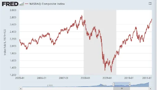
As we can see from the Figure 2.5, the index of the Nasdaq composite fluctuated from 2005 to 2011. More specifically, at firstly, the basic trend of the index had been going up before November 2007, meanwhile, the index reached the peak at 2,780.42 in October 2007. After that, the index started to fall down, and it plunged to 1,432.23 in March 2009, which was the bottom of the index during the global financial crisis. Therefore, the global financial crisis of 2007 had a huge influence on financial markets.
There are three main causes, which gave rise to the global financial crisis of 2007. The first point with respect to this is that easy credit conditions were existing in the financial markets. More specifically, the lower interest rates encourage borrowing while banks borrowed funds to investment firms, caused that the potential returns from investment rose and then the
banks were overleveraged to create a higher risk of bankruptcy. Moreover, the deregulation indicates that the insufficient regulation to guard against excessive risk-taking in the financial system. Additionally, sub-prime lending refers to the credit quality of particular borrowers, and the sub-prime borrowers have weakened credit histories and a greater risk of loan default than prime borrowers. Overall, all of causes worked to give rise to higher demand and price of house, and then the real estate pricing bubbles generated, therefore, the financial crisis broken out.
Figure 2.5 The Nasdaq Composite Index from 2005 to 2011 (1971=100)
Source: https://fred.stlouisfed.org/series/NASDAQCOM
To summary, the financial crisis, producing in one financial market, would also influent other financial markets.
2.3 Characteristics of Financial Time Series
Frequent volatility is a characteristic of financial time series in the stock market. In one ward, the volatility describes the account of risk or uncertainly about the changes’ size in a value of security. Generally, the higher the volatility exists, the risker the security is. Therefore, analyzing the volatility is useful to comprehend the stock market. This subchapter will show you the features of the volatility, which include volatility clustering, leptokurtic distribution and leverage effect, from these three characteristics, it will be clearly why volatility is important (Franke and Hafner, 2011).
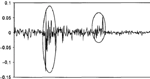
2.3.1 Volatility Clustering
Volatility of price in the stock market usually relates to time series. Sometimes the price is fairly stable, sometimes the volatility of price is fierce, so that the return keeps persistently high or low during a certain period. In sum, this phenomenon was general called “volatility clustering”. Benoit Mandelbrot (1963) had described the volatility clustering that “large changes tend to be followed by large changes, of either sign, and small changes tend to be followed by small changes.” And here has a quantitative expression of this fact that an autocorrelation function, which is significant and slowly decaying, showing as
𝑐𝑜𝑟𝑟(|𝑟𝑡|, |𝑟𝑡+𝜏|) > 0, where the |𝑟𝑡| is an absolute return, and the 𝜏 is a time lag. Figure 2.6 Volatility clustering phenomenon of financial time series
Source: by Alexander, C. (2001)
As illustrated in the Figure 2.6, the circles are indicating the low and high volatility which denote the spread autocorrelation. It is clearly to obverse that there has the trend of sustained periods of high or low volatility.
2.3.2 Leptokurtic Distribution
The leptokurtic distribution is a case of kurtosis that represents the attribute of flatness or peakedness of a distribution. Hence, in a leptokurtic distribution there are many scores close to the mean with few scores outlying symmetrically on both sides of central tendency.
It is worth nothing that the kurtosis of a normal distribution is 3, which means it is called leptokurtic distribution if the kurtosis is higher than 3, and it is platykurtic distribution when
the kurtosis is lower than 3.
The Figure 2.7 illustrates the comparison between the leptokurtic distribution and normal distribution straightforward. There has more returns clustered around the mean in the leptokurtic distribution.
Figure 2.7 Leptokurtic distribution and normal distribution
Source: by Luc, B. (2012)
2.3.3 Leverage Effect
The leverage effect is indicated as a negatively tendency between an asset’s volatility and the asset’s returns. Typically, the asset’s volatility declines due to the rising asset price, and vice versa. And as noted by Engle, R. (1993), that “Negative returns seemed to be more important predictors of volatility than position returns. Large price declines forecast greater volatility than similarly large price increases.” In brief, compared with a stock price increasing, there is a larger volatility when the stock price declines.
Normally, it is allowed to parametrize the leverage effect with assuming that the volatilities are functions of price levels when stochastic volatility models are used. There are four steps to estimate the leverage parameter:
a) firstly, define the quantities which are to be estimated,
𝜌(𝑡)𝑑𝑡 = 〈𝑑𝑋(𝑡), 𝑑𝜎2(𝑡)〉, 𝛾2(𝑡)𝑑𝑡 = 〈𝑑𝜎2(𝑡), 𝑑𝜎2(𝑡)〉, ∀𝑡 ∈ [0, 𝑇];
b) then, the volatility of the volatility and the leverage parameters can be estimated due to these quantities,
c) it can be obtained that,
𝜉𝜂 = 𝜌(𝑡)
𝜎2(𝑡);
d) using b) and c) to estimate the leverage parameter(𝜂).
Figure 2.8 Predicted stock volatility and effects of leverage
Source: by William, G. (1989)
Figure 2.9 Variance impact curve for the market portfolio
Source: by Bekaert, G. and Wu, G. (1997)
on daily data and changing financial leverage influents the level of stock return volatility from 1900 to 1987. Here, the effect of leverage is calculated by a time series of aggregate firm value divided by stock value, which has the same mean as the predictions of volatility from the regression model.
The Figure 2.9 illustrates how the market shock affects the market variance with or without the leverage level.
3 Methodology
The objective of this thesis is using the volatility spillover effects to analyze the interrelationship among the European equity markets. Therefore, the essential stuff is comprehending what the volatility spillover effect is, and how the volatility spillover effect works. Whatever, it will be expressed in this chapter.
In the first subchapter, the basic information of the volatility spillover effect will be described clearly. Moreover, there is a brief account of the literature relating to the volatility spillover effects, it will make readers clearer where the effects from, and if the one wants to know more, he/she can find the original literatures. The most vital parts in this chapter are describing the price spillover using VAR model and ARCH model. About VAR model, it will be indicated from the fundamental interpretation, the stationarity, and the advantages and disadvantages. There will have four main sorts of ARCH models will be illustrated, which are ARCH model, GARCH model, AR/GARCH model and EGARCH model (Bauwens et al, 2012). There still have some kinds of GARCH models – MGARCH model, etc., but they will not be used in this work, therefore they will not be described.
3.1 Volatility Spillover Effect and Its Importance
In this age of change, the human society is progressing rapidly on various fields. The financial market integration has become especially relevant over the last two decades. In addition, the substantial development of technology has allowed information to be conveyed more freely through global financial markets than ever before. The linkages between different stock markets in different region have grown stronger. Therefore, it is significant for portfolio managers and financial institutions that understanding the linkages between different financial markets. As volatility is measured by variance or standard deviation of returns, the researchers always use it to measure the total risk of financial assets (Brooks, 2002). Therefore, not only were the return causality linkages investigated, but also volatility spillover effect was measured. Volatility spillover effect is often used as a measure of the value at risk and hedging strategies of financial assets. Nowadays, as the emerging markets are becoming more and more important, economists start to pay attention to the emerging markets instead of only focus on developed counties (ex: The United State, Japan, the Britain, and etc.). For instance, in the stock markets, the degree of linkages between the emerging stock markets and developed stock markets has a significant effect to the investors who come from the developing or developed countries.
The liberalization of financial markets and capital flows are more integrated than ever before due to the progresses in the information spreading and trading technology. It is obviously both in developing and developed countries. The isolation domestic market would be reduced with management of the global news and trading of international finance. Moreover, those factors contribute to the single market to react to the news and shacks generated from other countries (Singh, Kumar, and Pandey, 2010). The linkage plays a pivotal role in pricing of domestic equites and international hedging strategy. The activities of the foreign cooperative partners would have a strong impact to domestic stock returns and volatilities with strong linkage while weak linkage contributes to hedging gain through diversification of international investing portfolio.
Figure 3.1 The volatility spillover in financial markets
Source: by Author
Volatility, which can be illustrated as a measure of fluctuation of price of a financial instrument with time, plays an increasingly key role in the financial markets. More and more researchers devote their attention to modeling and forecasting the volatility of financial returns for understanding its meaning and optimizing the financial decisions.
Currently, the volatility spillover effect is an important aspect of volatility. It indicates that a market volatility is influenced not only by itself but also by volatility coming from other market, as showing in the Figure 3.1. for instance, the financial crisis in the American in 2008 led to a huge wave of returns in the rest of the world. Moreover, the volatility spillover effect
is an extensive existence in different types of financial markets. Meanwhile, the volatility spillover effect can stimulate the process of volatility transmission from one financial market to another.
3.2 Literature Review
The study of financial market integration that a movement in one market would affects a movement in others is significant to investors and portfolio theories. Modeling volatility, which is in financial time series, has been paid much attention since the introduction of the Autoregressive Conditional Heteroskedasticity (ARCH) model of Engle (1982). Following Ross (1989) and Chan, Chan and Karolyi (1991) provided evidences that “it is the volatility of an asset’s price, and not the asset’s simple price change, that is related to the rate of flow of information to the market.” After that, there was a great deal of literature evaluating volatility spillover across financial markets from different countries. Janakiramanan and Lamba (1998) made a view that portfolios were invested in proximity of the domestic while the market also tend to influence one another due to the closely geography and economy. Moreover, the integration is a consequence of more familiar political and economic cooperation through the middle of countries (Johansson and Ljungwall, 2009).
It is obvious that stock market integration among developed counties was caused great concern at that time. Theodosssiou and Lee (1993) used a multivariate GARCH model to censor the nature and degree of independence of stock matket of the U.S., Britain, Germany, Japan, Canada, then they found that it was existed from the U.S. stock markets to others that statistically significant mean spillovers. Since the European Union (EU) is a free trade and monetary body of 27-member countries, the financial markets integration among different European countries has been generating. Therefore, numerous researchers have studied the linkages of stock markets between different European countries as the strong policy coordination and economic ties between EU and European Monetary Union (EMU). Gelos and Sahay (2000) argue that the geographic variations among the various national stock markets are changing less and less obvious with financial innovation, the advance of international finance and global integration. Furthermore, Harrison and Moore (2009) conducted an investigation of co-movement in stock markets between the developed markets of Western Europe and the developing markets of Central and Eastern Europe. Bubak, Kocenda and Zikes (2011) found the evidence of statistically significant volatility spillovers among foreign exchange markets in the Central Europe through studied dynamics of the volatility transmission
between the Central European currencies and the foreign exchange of EUR/USD that used model-free estimates of daily exchange rate volatility, which based on intraday data.
It should be clearly that even the Sims, C. (1980) put forward the Vector Autoregressions (VAR) model, it was utilized by Singh (2010) that the price spillover effects were estimated by VAR model. Moreover, using the three steps of AR/EGAECH model to estimate the volatility spillover effects was put forward by Christiansen, C. (2007).
Nevertheless, there are extensive studies described the relationship between the stock price and the volatility spillover effect. However, the studies of comparing the Western, Central and Eastern European stock markets were not that much. With the changing of the European financial market, a detailed study of its interrelation of stock markets is timely.
3.3 Univariate Volatility Models
The analysis of the financial time series indicated that there are three main characters of the rate of return of the financial time series – volatility clustering, leptokurtic distribution and leverage effect, which are non-classical phenomenon. Therefore, the homoscedasticity cannot be satisfied with the traditional econometric method, a severe result of the financial time series would be caused with modeling and statistic inference by traditional regression model. Due to that, Engle (1982) put forward a different view of Autoregressive Conditional Heteroskedasticity (ARCH) model, following Bollerslev (1986) did a simple and direct linear scalability to generating the Generalized Autoregressive Conditionally Heteroskedastic (GARCH) model. After that, more and more transformation of the ARCH generated.
In this subchapter the ARCH, GARCH, AR/GARCH, EGARCH models will be described (Rachev et al., 2007).
3.3.1 ARCH Model
The ARCH model can detect the variation of the financial data form one period to another one effectively. Hence, the ARCH model has been widely used to describe the volatility of the variables between finance and capital market, especially stock price, exchange rate, price of forward etc., following is the process:
𝑌𝑡 = 𝑸𝑡𝜷 + 𝜀𝑡, (3.1)
𝜀𝑡|𝜙𝑡−1~𝑁(0, ℎ𝑡), (3.2)
Where, 𝑡 = 1,2,3 … 𝑇; 𝑌𝑡 is the explained variable at time 𝑡, and the 𝑄𝑡 is the explanatory variable at time 𝑡; 𝜀𝑡 is white noise with 𝑉(𝜖) = 𝜎2; 𝜙𝑡 is the information set available at time
𝑡; ℎ𝑡is the conditional variance. Moreover, formulas can be described as:
𝑌𝑡= 𝜙1𝑌𝑡−1+ 𝜙2𝑌𝑡−2+ ⋯ + 𝜙𝑝𝑌𝑝−1+ 𝜀𝑡, (3.4)
ℎ𝑡= 𝑎0+ 𝑎1𝜀𝑡−12 + ⋯ + 𝑎
𝑞𝜀𝑡−𝑞2 , (3.5)
𝜀𝑡 = √ℎ𝑡𝑣𝑡. (3.6) Where, 𝑎0 > 0, 𝑎𝑡 ≥ 0(𝑖 = 0, ⋯ , 𝑞), 𝐸(𝑣𝑡) = 0, 𝐸(𝑣𝑡2) = 1. As be shown in the equation (3.5), the ℎ function is 𝑞-th order linear (in the squares), and the model, we are summarizing is the first-order linear model of the ARCH model. The error terms, 𝜀𝑡, are unconditional fat-tail distribution, meanwhile, the conditional variance, ℎ𝑡, can reflect the specialty of the changes of variables in the financial markets that “large and small errors tend to cluster together (in contiguous time periods)” by McNees (1979). Moreover, as be shown in equation (3.5), it is obvious that the various of the 𝜀𝑡 is decided by 𝜀𝑡−12 to 𝜀
𝑡−𝑞2 , therefore the various of the 𝜀𝑡 would be huge if the 𝜀𝑡−1 is huge, which means that the 𝜀𝑡−1 has a positive effect on future volatility in the market while the value of 𝑞 decided the duration of a random variable. The higher the 𝑞 is, the longer the duration has. The phenomena of volatility clustering are common in financial markets, especially the volatility of stock yield.
Even though the ARCH model has numerous advantages, there still have some disadvantages of it.
a) The model assumes that positive and negative shocks have the same effects on volatility. In practice, it is well known that asset prices respond differently to positive and negative shocks. b)ARCH model is comparatively restrictive. For example, in an ARCH (1) model, the 𝑎1
must be in (1, 1
√3) for a limited fourth moment. The constraint becomes complicated for higher order ARCH model.
c) Unless 𝑞 is huge, volatility maintains relatively short amount during a specific period.
3.3.2 GARCH Model
The equation (3.5) illustrates the distributed lags model of ℎ𝑡. The method, the lagged terms of ℎ𝑡 joined, generated for against an excess of the lagged terms of 𝜀𝑡2. Bollerslev (1986) got GARCH model due to the ARCH model, which allows for more flexible lag structure.
According to the ARCH process, just changing the structure of (3.5), we can get the process of GARCH (𝑝, 𝑞).
ℎ𝑡 = 𝑎0+ 𝑎1𝜀𝑡−12 + ⋯ + 𝑎 𝑞𝜀𝑡−𝑞2 + 𝜃1ℎ𝑡−1+ ⋯ 𝜃𝑝ℎ𝑡−𝑝, = 𝑎0+ ∑ 𝑎𝑖𝜀𝑡−𝑖2 𝑞 𝑖=1 + ∑ 𝜃𝑗ℎ𝑡−𝑗 𝑝 𝑗=1 , = 𝑎0+ 𝑎(𝐿)𝜀𝑡2+ 𝜃(𝐿)ℎ𝑡. (3.7) Where, 𝑝 ≥ 0, 𝑞 ≥ 0; 𝑎0 ≥ 0, 𝑎𝑖 ≥ 0, 𝑖 = 1, ⋯ , 𝑞; 𝜃𝑗 ≥ 0, 𝑗 = 1, ⋯ , 𝑝.
The GARCH (𝑝, 𝑞) should be kept as wide-sense stationary, hence, the 𝑎(𝐿) + 𝜃(𝐿) < 1. The conditional variance is a linear function of past sample variance only in the ARCH(𝑞)
process, however, the lagged conditional variance is allowed in the GARCH (𝑝, 𝑞) process as well. Moreover, this not hard to find that when 𝑝 = 0, the GARCH (0, 𝑞) is ARCH (𝑞), and when 𝑝 = 𝑞 = 0, the 𝜀𝑡 is a simply white noise.
In the GARCH model, there has a basic requirement that the white noise, 𝜀𝑡, denote a real-valued discrete-time stochastic process and the average of the 𝜀𝑡 is naught. Sometimes the regression equation could not adequately fetch the information of 𝜀𝑡. the residual sequence may have the autocorrelation instead of stochastic process. Based on the above, the first step is checking if the regression model of resident has homoscedasticity. If it does not have, the GARCH model can be used. The process on the above form the AR(𝑚)/GARCH(𝑝, 𝑞) model.
𝑌𝑡 = 𝜙1𝑌𝑡−1+ 𝜙2𝑌𝑡−2+ ⋯ + 𝜙𝑝𝑌𝑝−1+ 𝜀𝑡, (3.8)
𝜀𝑡 = ∑𝑚𝑘=1𝛽𝑗𝜀𝑡−𝑘+ 𝑣𝑡, (3.9)
𝑣𝑡 = √ℎ𝑡𝑒𝑡, (3.10)
ℎ𝑡= 𝑎0+ 𝑎(𝐿)𝜀𝑡2+ 𝜃(𝐿)ℎ
𝑡. (3.11) Where, the 𝑉𝑎𝑟(𝑣𝑡) = ℎ𝑡, and 𝑒𝑡~𝑁(0,1).
3.3.3 The
𝐆𝐀𝐑𝐂𝐇(𝟏, 𝟏)
Model
The GARCH(1,1) process is the simplest but useful GARCH process to do financial analysis. The GARCH(1,1) model is indicated as:
ℎ𝑡 = 𝑎0+ 𝑎1𝜀𝑡−12 + 𝜃1ℎ𝑡−1, (3.12) where, 𝑎0 > 0, 𝑎1 ≥ 0, 𝜃1 ≥ 0. Moreover, 𝑎1+ 𝜃1 < 1 cause the process is wide-sense stationarity. There is a theorem of the GARCH(1,1) process.
𝜇(𝑎1, 𝜃1, 𝑚) = ∑ (𝑚𝑗) 𝑐𝑗𝑎1 𝑗
𝜃1𝑚−𝑗
𝑚
𝑗=0 < 1, (3.13) where, 𝑚 is a positive integer; 𝑐0 = 1; 𝑐𝑗 = ∏𝑗𝑗=1(2𝑗 − 1), (𝑗 = 1,2 ⋯ 𝑚). And the 2𝑚-th moment can be showed as,
𝐸(𝜀𝑡2𝑚) = 𝑐𝑚[∑𝑚−1𝑛=0 𝑐𝑛−1𝐸(𝜀𝑡2𝑛)𝑎0𝑚−𝑛(𝑚−𝑛𝑚 )𝜇(𝑎1, 𝜃1, 𝑛)] × [1 − 𝜇(𝑎1, 𝜃1, 𝑚)]−1, (3.14) where the proof of this theorem shows in Bollerslev (1986).
Therefore, the coefficient of kurtosis of the GARCH(1,1) can be calculated. Moreover, the fourth-order moment should be used to calculate the calculation of the kurtosis, hence,
𝑘 = (𝐸(𝜀𝑡4) − 3𝐸(𝜀
𝑡2)2)𝐸(𝜀𝑡2)−2
= 6𝑎12(1 − 𝜃
12 − 2𝑎1𝜃1− 3𝑎12)−1. (3.15) There is an assumption that the kurtosis is greater than naught. Therefore, the GARCH(1,1)
process is leptokurtic.
3.3.4 EGARCH Model
According to above, it is obviously that there are some limitations in the GARCH model. If the coefficients of the model are negative, GARCH model could not be used. Moreover, GARCH model also cannot give the explanation for leverage effects. Besides, the feedback between conditional variance and mean cannot be do directly in the GARCH model.
Because of those reasons, Nelson (1991) put forward an asymmetric GARCH model, which is called exponential GARCH or EGARCH model, commonly represents below:
{ 𝜀𝑡= 𝜎𝑡𝜂𝑡 𝑙𝑛𝜎𝑡2 = 𝜔 + ∑ 𝛼 𝑖𝑔(𝜂𝑡−𝑖) + ∑ 𝛽𝑗𝑙𝑛𝜎𝑡−𝑗2 𝑝 𝑗=1 𝑞 𝑖=1 𝑔(𝜂𝑡) = 𝜃𝜂𝑡+ 𝛾[|𝜂𝑡| − 𝐸(|𝜂𝑡|)] , (3.16) where, {𝛼𝑖}, 𝑖 = 1,2, ⋯ , 𝑞, {𝛽𝑗}, 𝑗 = 1,2, ⋯ , 𝑝 are nonrandom and real scalable series; moreover, 𝑔( ∙ ) should be satisfied with 𝐸𝑡−𝑖(𝑔(𝜂𝑡)) = 0. It is easy to be observed when 𝜃 <
0, with the same size of volatility, the amplification of conditional variance with negative fluctuation is surpass than with positive fluctuation, which expresses asymmetry. In practice, the equation (3.16) could be simplified as:
𝑙𝑛𝜎𝑡2 = 𝜔 + ∑ (𝜃 𝑖| 𝜀𝑡−𝑖 𝜎𝑡−𝑖| + 𝛾𝑖 𝜀𝑡−𝑖 𝜎𝑡−𝑖) + ∑ 𝛽𝑗𝑙𝑛𝜎𝑡−𝑗 2 𝑝 𝑗=1 𝑞 𝑖=1 . (3.17)
Specially, in the EGARCH(1,1) model, the conditional variance equation is:
𝑙𝑛𝜎𝑡2 = 𝜔 + 𝜃1|𝜀𝑡−1
𝜎𝑡−1| + 𝛾1
𝜀𝑡−1
𝜎𝑡−1+ 𝛽1𝑙𝑛𝜎𝑡−1
2 . (3.18) The EGARCH(1,1) model is usually used to discuss the asymmetric effect of the prices in
stock markets. In the equation (3.16), when 𝛾 ≠ 0, it means the distraction is asymmetric to effect of stock price; by contrast, when 𝛾 < 0, the negative exogenous shock surpasses than positive exogenous shock about affecting the price of financial products, 𝛾, here, is called leverage effect.
The parameter estimation of the EGARCH model is commonly got by method of maximum likehood, the distribution of {𝜂𝑡} do not only adopt the standardized normal distribution (𝜂~𝑁(0,1)), but also use generalized error distribution (GED) with a mean of zero and a variance of one, the density of GED is given by:
𝑓(𝜂𝑡) =𝜈𝑒𝑥𝑝[−
1 2|𝜂𝑡⁄ |𝜆
𝜈]
𝜆2(1+1 𝜈⁄ )Γ(1 𝜈⁄ ),
where, −∞ < 𝜂𝑡< +∞, 0 < 𝜈 ≤ ∞, Γ( ∙ )is a gamma function, and
𝜆 = [2−2 𝜈⁄ Γ(1 𝜈⁄ )⁄Γ(3 𝜈⁄ )]
1 2 ⁄
.
When 𝜈 = 2, 𝜆 = 1, {𝜂𝑡} has a standardized normal distribution. For 𝜈 < 2, the distribution of
{𝜂𝑡} has thicker tails than normal, the kurtosis is higher than 3; nevertheless, for 𝜈 > 2, the distribution of {𝜂𝑡} has thinner tails than normal, and
𝐸|𝜂𝑡| =𝜆21 𝜈⁄ Γ(2 𝜈⁄ )
Γ(1 𝜈⁄ ) .
The difference between the EGARCH model and GARCH model:
a) The volatility of EGARCH model, measured by conditional variance (𝜂𝑡), is a specific multiplicative function of lagged innovations. By contrast, volatility of GARCH model is an additive function of the lagged error term of 𝜀𝑡2.
b)The positive and negative things are able to have asymmetrical volatility.
In summary, because the EGARCH model do not have parameter restrictions, the probability of instability of optimal routines is declined.
3.4 Price Spillover Model – VAR model
Christopher Sims (1980) described a new flexible and tractable framework for analyzing financial time series, which is named as Vector Autoregressions (VAR) model. While a VAR is a 𝑛-variable linear model with 𝑛-equations in which each variable is explained by its own lagged values, moreover it also be explained by current and past values of the remaining 𝑛 − 1
variables, a common autoregression is a single-variable linear model, using lagged values of a variable to explain its own.
𝒚𝑡 = 𝒄 + 𝝓1𝒚𝑡−1+ ⋯ + 𝝓𝑝𝒚𝑡−𝑝+ 𝝐𝑡, (3.19) where 𝒚𝑡: (𝑁 × 1); 𝝓𝑖: (𝑁 × 𝑁); 𝝐𝑡: (𝑁 × 1);
𝐸(𝝐𝑡) = 0; 𝐸(𝝐𝑡𝝐′𝜏) = {𝛀 𝑡 = 𝜏
𝟎 𝑡 ≠ 𝜏 (𝛀 positive definite matrix).
A VAR model is model with a vector generalization of a scalar autoregression. Moreover, each variable is regressed not only on 𝑝 lags of its own but on 𝑝 of other variables lags as well.
[𝑰𝑁− 𝝓1𝐿 − ⋯ − 𝝓𝑝𝐿𝑝]𝒚𝑡 = 𝒄 + 𝝐𝑡
𝝓(𝐿)𝒚𝑡 = 𝒄 + 𝝐𝑡, (3.20) where, 𝝓(𝐿)(𝑁 × 𝑁) is a matrix polynomial of 𝐿 and the element (𝑖, 𝑗) is a scalar polynomial in 𝐿. Overall, it can be called unrestricted VAR model if there is equation (3.19) or (3.20).
In the VAR model, as every equation has lagged values of endogenous variables and they have no connection with 𝝐𝑡, the Ordinary Least Square Method (OLS) could be used to forecast the right-hand side of every equation in turn. The VAR model will be applied to estimate the price spillover effect, and this approach was utilized for instance by Singh (2010).
3.4.1 The Stationarity of VAR Model
When a pulsation impact is put on one equation of the VAR model, if the strike will disappear gradually, which means the system is stable, and vice versa.
Following is the example of first-order VAR model,
𝒚𝑡 = 𝒄 + 𝝓1𝒚𝑡−1+ 𝝐𝑡, (3.21) when 𝑡 = 1, there is
𝒚1 = 𝒄 + 𝝓1𝒚0+ 𝝐1, (3.22) when 𝑡 = 2, with the iterative analysis using, the formula is got,
𝒚2 = 𝒄 + 𝝓1𝒚1 + 𝝐2 = 𝒄 + 𝝓1(𝒄 + 𝝓1𝒚0+ 𝝐1) + 𝝐2
= (𝑰 + 𝝓1)𝒄 + 𝝓12𝒚0+ 𝝓1𝝐1+ 𝝐2, (3.23) when 𝑡 = 3, the formula is
𝒚3 = 𝒄 + 𝝓1𝒚2+ 𝝐3 = 𝒄 + 𝝓1[(𝑰 + 𝝓1)𝒄 + 𝝓12𝒚0+ 𝝓1𝝐1+ 𝝐2] + 𝝐3
= (𝑰 + 𝝓1+ 𝝓12)𝒄 + 𝝓13𝒚0+ 𝝓12𝝐1+ 𝝓1𝝐2+ 𝝐3, (3.24) above all, the general formula is
𝒚𝑡= (𝑰 + 𝝓1+ 𝝓12+ ⋯ 𝝓1𝑡−1)𝒄 + 𝝓1𝑡𝒚0+ ∑𝑡−1𝑖=0𝝓1𝑖𝝐𝑡−𝑖. (3.25) According to the equation (3.25), the independent value 𝑦𝑡 has the relationship with vector c, vector 𝒚0, and vector 𝝐𝑡, it depends on the result after strikes of that three vectors that the system is stable or not.
If the VAR system is stable, the conclusions are:
a) If 𝑡 = 1, putting a unit strike on 𝒄, when time reached to 𝑡, the effect is
(𝑰 + 𝝓1+ 𝝓12 + ⋯ 𝝓1𝑡−1). When 𝑡 → ∞, the effect is a limited value, which is (𝑰 − 𝝓1)−1.
b)If putting a unit strike on 𝒚0, the effect will be 𝝓1𝑡 when time is 𝑡. Moreover, if 𝑡 →
∞, 𝝓1𝑡→ 0, the effect vanished.
c) Observing ∑𝑡−1𝑖=0𝝓1𝑖𝝐𝑡−𝑖, the further the strike of white noise is, the lower the effect is. Through the analysis of first-order equation, it is easy to get that autoregression process has a long memory ability to pulsation impact of innovation. Similarly, if the response of the endogenous variable will not disappear over time with a pulsation impact of innovation, it is the non-stationary process of VAR model.
3.4.2 Advantages and Disadvantages of VAR Model
The VAR model is a popular macroeconomic framework, numerous researchers would like to use it. Why is it fairly popular? There will be three main reasons below:
a) Since all variables in the VAR model are endogenous, it is not necessary to specify which variable is exogenous or endogenous.
b)The VAR model, which allows the value of a variable to depend on more than its own lags or combinations of white noise terms, is more general than ARMA model.
c) The OLS can be used on each equation, as there are no contemporaneous terms on the right-hand side of the equations.
Even though the VAR model has a vast number of advantages, there still have some weaknesses of it.
a) The VAR model is a theoretical model, it is hard to practice. b)It is not easy to decide the proper lag length.
c) There are many parameters. For instance, if there are 𝑥 equations for 𝑦 variables, and the lag is 𝑘, there are (𝑔 + 𝑘𝑔2) parameters that should be estimated.
d)It is hard to ensure if all components of the VAR model need to keep stationary. Overall, the VAR model still is an essential instrument in macroeconomic research.
3.5 Volatility Spillover Models – AR/EGARCH model
between the American and European bond market by Christiansen (2007). In this thesis, the same approach as above will be applied.
Firstly, the American return was got from a univariate AR/GARCH (1,1) model. Then, the univariate AR/GARCH (1,1) model was used to estimate the aggregate European return with an extended version. Besides, the return for individual European stock market was estimated by the extended univariate AR/GARCH (1,1) model. However, Nelson (1991) indicated that the constraints parameters of the GARCH model has to be positive as well as the size of volatility had no relationship with the sign of unexpected return. Thus, the GARCH model is not able to distinguish the leverage effect on volatility. Hence, for explaining the leverage effect, the EGARCH model will be used to instead of GARCH model in this thesis, in which using the AR/EGARCH (1,1) model to investigate the effects of the chosen stock markets.
Firstly, the American return is shown as:
𝑅𝑢𝑠,𝑡 = 𝜙0,𝑢𝑠+ 𝜙1,𝑢𝑠𝑅𝑢𝑠,𝑡−1+ 𝜀𝑢𝑠,𝑡, (3.26) where, 𝜀𝑢𝑠,𝑡~𝑁(0, 𝜎𝑢𝑠,𝑡2 ), 𝜎
𝑢𝑠,𝑡2 is the conditional variance of the American stock market. 𝜙1,𝑢𝑠 represses the lagged return of the American return influent itself. And according to the EGARCH (1,1) model, the conditional variance is
𝑙𝑛𝜎𝑢𝑠,𝑡2 = 𝜔𝑢𝑠,𝑡+ 𝜃1,𝑢𝑠|𝜀𝑢𝑠,𝑡−1
𝜎𝑢𝑠,𝑡−1| + 𝛾1,𝑢𝑠
𝜀𝑢𝑠,𝑡−1
𝜎𝑢𝑠,𝑡−1+ 𝛽𝑢𝑠𝑙𝑛𝜎𝑢𝑠,𝑡−1
2 . (3.27) where, 𝛽𝑢𝑠 is the persistence of volatility, 𝛾1,𝑢𝑠 controls the leverage effect on volatility by positive or negative returns. More specifically,
{ 𝜀𝑢𝑠,𝑡−1 𝜎𝑢𝑠,𝑡−1> 0, 𝑚𝑒𝑎𝑛𝑠 𝑡ℎ𝑒 𝑒𝑓𝑓𝑒𝑐𝑡 𝑜𝑓 𝑡ℎ𝑒 𝑠ℎ𝑜𝑐𝑘 𝜀𝑢𝑠,𝑡−1 𝑖𝑠 (𝜃1,𝑢𝑠+ 𝛾1,𝑢𝑠) ( 𝜀𝑢𝑠,𝑡−1 𝜎𝑢𝑠,𝑡−1) 𝜀𝑢𝑠,𝑡−1 𝜎𝑢𝑠,𝑡−1< 0, 𝑚𝑒𝑎𝑛𝑠 𝑡ℎ𝑒 𝑒𝑓𝑓𝑒𝑐𝑡 𝑜𝑓 𝑡ℎ𝑒 𝑠ℎ𝑜𝑐𝑘 𝜀𝑢𝑠,𝑡−1 𝑖𝑠 (𝜃1,𝑢𝑠− 𝛾1,𝑢𝑠) ( 𝜀𝑢𝑠,𝑡−1 𝜎𝑢𝑠,𝑡−1) 𝜀𝑢𝑠,𝑡−1 𝜎𝑢𝑠,𝑡−1= 0, 𝑚𝑒𝑎𝑛𝑠 𝑡ℎ𝑒 𝑣𝑎𝑟𝑖𝑎𝑛𝑐𝑒 𝑡𝑜 𝑠ℎ𝑜𝑐𝑘𝑠 𝑖𝑠 𝑠𝑦𝑚𝑚𝑡𝑟𝑖𝑐 .
Moreover, the aggregate European return is shown as:
𝑅𝐸𝑈,𝑡 = 𝜙0,𝐸𝑈+ 𝜙1,𝐸𝑈𝑅𝐸𝑈,𝑡−1+ 𝜑𝐸𝑈𝑅𝑢𝑠,𝑡−1+ 𝜇𝐸𝑈𝜀𝑢𝑠,𝑡 + 𝜀𝐸𝑈,𝑡, (3.28) As can be seen from the equation (3.28), its own lagged return and the American lagged return influent the aggregate European return. Furthermore, 𝜑𝐸𝑈 and 𝜇𝐸𝑈 estimate the return and volatility spillover effect from the American stock market to Eurozone stock market respectively. And according to the EGARCH (1,1) model, the conditional variance is
𝑙𝑛𝜎𝐸𝑈,𝑡2 = 𝜔 𝐸𝑈,𝑡+ 𝜃1,𝐸𝑈| 𝜀𝐸𝑈,𝑡−1 𝜎𝐸𝑈,𝑡−1| + 𝛾1,𝐸𝑈 𝜀𝐸𝑈,𝑡−1 𝜎𝐸𝑈,𝑡−1+ 𝛽𝐸𝑈𝑙𝑛𝜎𝐸𝑈,𝑡−1 2 . (3.29) The individual European stock market is shown as:
𝑅𝑖,𝑡 = 𝜙0,𝑖+ 𝜙1,𝑖𝑅𝑖,𝑡−1+ 𝜑𝑖𝑅𝑢𝑠,𝑡−1+ 𝛿𝑖𝑅𝐸𝑈,𝑡−1+ 𝜇𝑖𝜀𝑢𝑠,𝑡+ 𝜓𝑖𝜀𝐸𝑈,𝑡+ 𝜀𝑖,𝑡, (3.30) where, 𝑖 = 1,2,3,4, which represents four chosen countries. The return of each country depends on its own lagged return, the American lagged return and European lagged return. 𝜑𝑖 and 𝜇𝑖 estimate the return and volatility effect from the American stock market, whereas the 𝛿𝑖 and
𝜓𝑖 measure the regional return and volatility effect. Besides, 𝜀𝑖,𝑡~𝑁(0, 𝜎𝑖,𝑡2), thus,
𝑙𝑛𝜎𝑖,𝑡2 = 𝜔𝑖+ 𝜃1,𝑖|𝜀𝑖,𝑡−1
𝜎𝑖,𝑡−1| + 𝛾1,𝑖
𝜀𝑖,𝑡−1
𝜎𝑖,𝑡−1+ 𝛽𝑖𝑙𝑛𝜎𝑖,𝑡−1
2 . (3.31) The unexpected return from each stock market is donated as:
𝑒𝑢𝑠,𝑡 = 𝜀𝑢𝑠,𝑡, (3.32)
𝑒𝐸𝑈,𝑡 = 𝜇𝐸𝑈𝜀𝑢𝑠,𝑡+ 𝜀𝐸𝑈,𝑡, (3.33)
𝑒𝑖,𝑡 = 𝜇𝑖𝜀𝑢𝑠,𝑡+ 𝜓𝑖𝜀𝐸𝑈,𝑡+ 𝜀𝑖,𝑡, (3.34)
𝜀𝑢𝑠,𝑡, 𝜀𝐸𝑈,𝑡 and 𝜀𝑖,𝑡 are assumed to be independent. Thus, the conditional variance of unexpected return in country 𝑖 can be indicated as:
ℎ𝑖,𝑡 = 𝐸(𝑒𝑖,𝑡2|𝐼𝑡−1) = 𝜇𝑖2𝜎𝑢𝑠,𝑡2 + 𝜓𝑖2𝜎𝐸𝑈,𝑡2 + 𝜎𝑖,𝑡2. (3.35) In addition, the variance ratio is able to detect which stock market affects the volatility more, the American stock market or the Eurozone stock market. The formulas are showing as:
𝑉𝑅𝑖,𝑡𝑢𝑠 = 𝜇𝑖2𝜎𝑢𝑠,𝑡2
ℎ𝑖,𝑡 , (3.36)
𝑉𝑅𝑖,𝑡𝐸𝑈 =𝜓𝑖2𝜎𝐸𝑈,𝑡2
ℎ𝑖,𝑡 . (3.37)
Except the influences from the American stock market and the Eurozone stock market, it also can be affected by itself,
𝑉𝑅𝑖,𝑡𝑖 = 1 − 𝑉𝑅𝑖,𝑡𝑢𝑠− 𝑉𝑅𝑖,𝑡𝐸𝑈 =𝜎𝑖,𝑡2
4 Data Sample Description
In this thesis, we will analysis and compare if the volatility of the American or Eurozone stock market have an effect on the volatility of French, German, British and Swiss stock markets. Therefore, a brief account of chosen stock markets will be in the first part. Then, descripting and analyzing the six stock indexes from six chosen stock markets respectively. Lastly, for the purpose of this thesis, the total time period is divided into three sub periods, and statistics in each period will be descripted.
4.1 Characteristics of Investigated Stock Markets
For the purpose of this thesis there were selected four important stock markets – French stock market and German stock market, which are European Union members; British stock market and Swiss stock market, which are not European Union members. Therefore, this subchapter will illustrate the fundamental information of those four stock markets.
4.1.1 French Stock Market
The Paris Bourse, also called Paris Stock Exchange, is an essential stock market in France. There are two other French stock markets – Financial Futures Market (MATIF) and the Financial Options Market (MONEP).
There are four different markets operated in Paris Bourse.
a) Firstly, it is the Official Stock Exchange, which is called Marche Official. The market is dedicated for comparatively large companies, on which at least 25% of their equity publicly held.
b)Then, it is the Second Market, which is called Second Marche. This market accepts those companies, which are not large enough to be traded in the Marche Official. It is considered as a temporary level for companies.
c) Moreover, it is the New Market, which is called Le Nouveau Marche. This market is intended for growth companies, e.g., small, young companies with high risk. Companies can list without a profitability or trading record.
d)Lastly, the Over-the-Counter Market, not a permanent market, is used for temporary transactions between non-listed companies.
4.1.2 German Stock Market
As one of the financial center in Euro areas, Germany has eight stock exchanges, which are sited in Frankfurt, Dusseldorf, Munich, Stuttgart, Hanover, Hamburg, and Bremen respectively. The Frankfurt Stock Exchange (FSE) is the largest stock exchange in Germany, accounting for approximately 75% of the total trading volume. It is a joint stock company in which the main shareholders are bank members. The Dusseldorf is the second largest one with representing about 10% of the trading volume. Therefore, these are just small parts of total trading volume to other stock exchanges.
There are different market segments in German stock exchanges. The first place is the regulated market, which is divided into prime standard and general standard. Moreover, the expected total market value of all shares must be over EUR 1.25 million if companies want to be listed in the regulated market, unless in which the shares of the same class were listed in the same stock market already. Then, it is the open market, which is divided into entry standard listing in the qualified open market and quotation board for secondary listings (unqualified open market). The companies have pay the share capital at least EUR 750,000 to be in this market.
4.1.3 British Stock Market
Speaking of British stock market, the London Stock Exchange (LSE) is an essential stock market in the Britain, which is called the International Stock Exchange of the United Kingdom and the Republic of Ireland formally. The LSE, playing an important role in the development of global capital markets, is one of the world’s largest and most international stock exchanges. The LSE provides the widest choices of routes to market, which are available to both UK and international companies. Moreover, there are about 3,000 companies from more than 70 counties that listed and traded on British stock market.
The key benefits of the LSE are:
a) It can provide access to capital for growth, meanwhile it is enable enterprises to raise finance for further development.
b)It can create market shares of the enterprise and broaden the shareholder base. c) It will place an objective market value on the business of enterprise.
d)It is capable to increase the ability of company to make acquisitions and use quoted shares as currency.
e) It can augment the loyalty of suppliers and customers.
Furthermore, the LSE runs three markets, which is showing below:
a) Firstly, it is about the Official List – the largest market, which is intended for large companies that have substantial public floating and a history of business activity. And this market is divided into an international section and a nation one, so that the non-British stocks can be traded on.
b)Secondly, Unlisted Securities Market, set up in 1980 to cater for smaller enterprises, has met only limited success. Nevertheless, it stopped allowing new companies listing and was closed at the end of 1996.
c) Lastly, the Alternative Investment Market, set up in 1995, is a new attempt to build a market for smaller companies. It does not have any requirements for minimum trading period or number of shares in the public compared with the Official List.
4.1.4 Swiss Stock Market
The SIX Swiss Exchange, established in 1993, is a central link in the value chain of the Swiss stock market. It organizes, operates and regulates significate factors of the capital market infrastructure, and it also provides extensive services on global ranges. Moreover, it is one of the four business areas of the SIX, which has: securities trading (SIX Swiss Exchange), financial information services (SIX Financial Information), payment services (SIX Payment Services) and securities services (SIX Securities Services). And there are 150 domestic and foreign shareholders joined in the SIX as owners.
The SIX is consistently developing its infrastructure for the Swiss financial center, and the Swiss financial center, which is attractive, diversified, and also has a remarkable international network, is one of the best in the world. The SIX propose to improve consistently as part of an active interlocution between Swiss market participants and authorities. Moreover, the Swiss authorities also support open markets in advance.
4.2 Description of Investigated Indexes
In this subchapter, six indexes - CAC 40, DAX 30, FTSE 100, SMI 20, EURO STOXX 50 and S&P 500 - from chosen counties and areas will be indicated and analyzed.
4.2.1 Paris Stock Index CAC 40
The CAC 40 is a benchmark French stock market index. It describes a capitalization-weighted measure of the 40 most important enterprises on the Euronext Paris. Moreover, the market capitalization had been €1457.5 billion until March 29, 20181. The most famous
companies, consisted the index, were AXA, L’Oréal, Atos, etc. Therefore, this thesis uses the CAC 40 Index to analysis French stock market.
The index value of CAC 40 Index is calculated as the result of the basic level multiplied by the sum of the prices multiplied by the corresponding weights and divided by the adjustment coefficient multiplied by the basis capitalization. The formula is shown below:
𝐼𝑡 = 1000 ×∑𝑁𝑖=1𝑄𝑖,𝑡𝐹𝑖,𝑡𝑓𝑖,𝑡𝐶𝑖,𝑡
𝐾𝑡∑𝑁𝑖=1𝑄𝑖,0𝐶𝑖,0
, (4.1) where, 𝑡 is day of calculation, 𝑁 is number of constituent equities in index, 𝑄𝑖,𝑡 is number of shares of equity 𝑖 on day 𝑡, 𝐹𝑖,𝑡 is free float of equity 𝑖, 𝑓𝑖,𝑡 is capping factor of equity 𝑖, 𝐶𝑖,𝑡 is price of equity 𝑖 on day 𝑡, 𝐾𝑡 is adjustment coefficient for base capitalization on day 𝑡, 𝑄𝑖,0 is number of shares of equity 𝑖 on index base data, 𝐶𝑖,0 is price of equity 𝑖 on index base day.
Chart 4.1 The CAC 40 Index from 01/01/2003 to 22/08/2017
2,000 2,500 3,000 3,500 4,000 4,500 5,000 5,500 6,000 6,500 03 04 05 06 07 08 09 10 11 12 13 14 15 16 17 CAC 40 Index Source: by Author
As can be seen from the Chart 4.1, the line chart shows the CAC 40 Index from the beginning of 2003 to the August of 2017 while the whole figures are divided into three
periods by two red lines with February 8, 2007 and July 30, 2009 respectively.
More specifically, before the former red line, the main trend of the line was consistently increase, and the line reached the bottom at around 2,400 points on March of 2003. In February 8, 2007, the line reached the peak at about 5,700 points in the first sub-period. Moreover, between the two red lines, there was a steadily decline basically with peaking at approximately 6,100 points on July of 2007 and bottoming out at approximately 2,500 points on February of 2009. After July 30, 2009, with a gradually upward trend basically, there were two substantial recessions – the former one was around May of 2011, when the index dropped from approximately 3,700 points to 2,600 points; the latter one was from April of 2015 to February of 2016, on which the index declined from approximately 5,200 to 3,900 points respectively.
As shown in the Chart 4.2, this line chart shows the returns of CAC 40 Index from the beginning of 2003 to the August of 2017 while the whole figures are divided into three sub-periods by two red lines with February 8, 2007 and July 30, 2009 respectively. More precisely, the volatility of returns between the two red lines was nearly five times as high as the returns before the former red line as well as nearly three times as high as the returns after the latter red line.
Chart 4.2 The CAC 40 Returns from 01/01/2003 to 22/08/2017
-.12 -.08 -.04 .00 .04 .08 .12 03 04 05 06 07 08 09 10 11 12 13 14 15 16 17 CAC 40 Returns Source: by Author
4.2.2 Frankfurt Stock Index DAX 30
blue-chip stock market index, measures the share performance