Gray-box inference for structured Gaussian process models
Pietro Galliani Amir Dezfouli Edwin V. Bonilla Novi Quadrianto
SMiLe CLiNiC University of Sussex
The University of New South Wales
The University of New South Wales
SMiLe CLiNiC University of Sussex
Abstract
We develop an automated variational infer-ence method for Bayesian structured predic-tion problems with Gaussian process (gp) priors and linear-chain likelihoods. Our ap-proach does not need to know the details of the structured likelihood model and can scale up to a large number of observations. Furthermore, we show that the required expected likelihood term and its gradients in the variational objective (ELBO) can be estimated efficiently by using expecta-tions over very low-dimensional Gaussian distributions. Optimization of the ELBO is fully parallelizable over sequences and amenable to stochastic optimization, which we use along with control variate techniques to make our framework useful in practice. Results on a set of natural language pro-cessing tasks show that our method can be as good as (and sometimes better than, in particular with respect to expected log-likelihood) hard-coded approaches includ-ing svm-struct and crfs, and overcomes the scalability limitations of previous infer-ence algorithms based on sampling. Over-all, this is a fundamental step to developing automated inference methods for Bayesian structured prediction.
1
INTRODUCTION
Developing automated inference methods for com-plex probabilistic models has become arguably one of the most exciting areas of research in machine Proceedings of the20thInternational Conference on Artifi-cial Intelligence and Statistics (AISTATS) 2017, Fort Laud-erdale, Florida, USA. JMLR: W&CP volume 54. Copyright 2017 by the author(s).
learning, with notable examples in the probabilistic programming community given bystan (Hoffman and Gelman, 2014) andchurch (Goodman et al., 2008). One of the main challenges for these types of approaches is to formulate expressive probabilistic models and develop generic yet efficient inference methods for them. From a variational inference per-spective, one particular approach that has addressed such a challenge is the black-box variational inference framework of Ranganath et al. (2014).
While the works of Hoffman and Gelman (2014) and Ranganath et al. (2014) have been successful with a wide range of priors and likelihoods, their direct application to models with Gaussian process (gp) priors is cumbersome, mainly due to the large num-ber of highly coupled latent variables in such models. In this regard, very recent work has investigated automated inference methods for general likelihood models when the prior is given by a sparse Gaus-sian process (Hensman et al., 2015b; Dezfouli and Bonilla, 2015). While these advances have opened up opportunities for applyinggp-based models well beyond regression and classification settings, they have focused on models with i.i.d observations and, therefore, are unsuitable for addressing the more challenging task ofstructured prediction.
Structured prediction refers to the problem where there are interdependencies between outputs and it is necessary to model these dependencies explic-itly. Common examples are found in natural lan-guage processing (nlp) tasks, computer vision and bioinformatics. By definition, observation models in these problems are not i.i.d and standard learn-ing frameworks have been extended to consider the constraints imposed by structured prediction tasks. Popular structured prediction frameworks are con-ditional random fields (crfs; Lafferty et al., 2001), maximum margin Markov networks (Taskar et al., 2004) and structured support vector machines (svm -struct, Tsochantaridis et al., 2005).
From a non-parametric Bayesian modeling perspec-tive, in general, and from agpmodeling perspective, in particular, structured prediction problems present very hard inference challenges because of the rapid explosion of the number of latent variables with the size of the problem. Furthermore, structured likeli-hood functions are usually very expensive to compute. In an attempt to build non-parametric Bayesian ap-proaches to structured prediction, Bratières et al. (2015) have proposed a framework based on a crf -type modeling approach withgps, and use elliptical slice sampling (ess; Murray et al., 2010) as part of their inference method. Unfortunately, although their method can be applied to linear chain structures in a generic way without considering the details of the likelihood model, it is not scalable as it involves sampling from the fullgpprior.
In this paper we present an approach for automated inference in structuredgpmodels with linear chain likelihoods that builds upon the structuredgpmodel of Bratières et al. (2015) and the sparse variational framework of Dezfouli and Bonilla (2015). In par-ticular, we show that the model of Bratières et al. (2015) can be mapped onto a generalization of the au-tomated inference framework of Dezfouli and Bonilla (2015). Unlike the work of Bratières et al. (2015), by introducing sparse gp priors in structured pre-diction models, our approach is scalable to a large number of observations. More importantly, this ap-proach is also generic in that it does not need to know the details of the likelihood model in order to carry out posterior inference. Finally, we show that our inference method is statistically efficient, as it only requires expectations over low-dimensional Gaussian distributions in order to carry out posterior approximation.
Our experiments on a set of nlp tasks, including noun phrase identification, chunking, segmentation, and named entity recognition, show that our method can be as good as (and sometimes better than, in par-ticular with respect to expected log-likelihood) hard-coded approaches including svm-struct and crfs, and overcomes the scalability limitations of previous inference algorithms based on sampling.
We refer to our approach as “gray-box” inference since, in principle, for general structured prediction problems it may require some human intervention. Nevertheless, when applied to fixed structures, our proposed inference method is entirely “black box”. For example, as we will see, we can replace the exact likelihood with a pseudo-likelihood without needing to make any other modifications to our code.
2
GAUSSIAN PROCESS MODELS
FOR STRUCTURED
PREDICTION
Here we are interested in structured prediction prob-lems where we observe input-output pairs D =
{Xn,yn} Nseq
n=1, where Nseq is the total number of ob-servations,Xn ∈ X is a descriptor of observationn andyn ∈ Yis a structured object such as a sequence, a tree or a grid that reflects the interdependences be-tween its individual constituents. Our goal is that of, given a new input descriptorX?, predicting its cor-responding structured labelsy?, and more generally, a distribution over these labels.
A fairly general approach to address this problem with Gaussian process (gp) priors was proposed by Bratières et al. (2015) based on crf-type models, where the distribution of the output given the input is defined in terms of cliques, i.e. sets of fully connected nodes. Such a distribution is given by:
p(y|X,f) = exp ( P cf(c,Xc,yc)) P y0∈Yexp ( P cf(c,Xc,y0c)) , (1)
where Xc andyc are tuples of nodes belonging to clique c; f(c,Xc,yc) is their corresponding latent variable; and f is the collection of all these latent variables, which are assumed to be drawn from a zero-meangpprior with covariance functionκ(·,·;θ), with
θbeing the hyperparameters. It is clear that such a model is a generalization of vanillacrfs where the potentials are draws from agpinstead of being linear functions of the features.
2.1 Linear chain structures
In this paper we focus on linear chain structures where the output corresponding to datapointnis a linear chain of lengthTn, whose corresponding con-stituents stem from a common set. In other words,
Xn is aTn×D matrix of feature descriptors andyn is a sequence ofTnlabels drawn from the same vocab-ularyV. In this case, in order to completely define the prior over the clique-dependent latent functions in Equation (1), it is necessary to specify covariance functions over the cliques. To this end, Bratières et al. (2015) propose a kernel that is non-zero only when
two cliques are of the same type, i.e. both are unary cliques or both are pairwise cliques. Furthermore, these kernels are defined as:
κun((t,xt, yt),(t0,x0t, yt0)) =I[yt=yt0]κ(xt,x0t) κbin((yt, yt+1),(yt0, yt0+1)) =I[yt=yt0∧yt+1=yt0+1],
whereκun is the covariance on unary functions and
κbinis the covariance on pairwise functions. With a suitable ordering of these latent functions, we obtain a posterior covariance matrix that is block-diagonal, with the first|V|blocks corresponding to the unary covariances, each of sizeTn; and the last block, cor-responding to the pairwise covariances, being a diag-onal (identity) matrix of size|V|2, where|V|denotes
the vocabulary size.
To carry out inference in this model, Bratières et al. (2015) propose a sampling scheme based on elliptical
slice sampling (ess; Murray et al., 2010). In the following section, we show an equivalent formulation of this model that leverages the general class of mod-els with i.i.d likelihoods presented by Nguyen and Bonilla (2014). Understanding structuredgpmodels from such a perspective will allow us to generalize the results of Nguyen and Bonilla (2014); Dezfouli and Bonilla (2015) in order to develop an automated variational inference framework. The advantages of such a framework are that of (i) dealing with generic likelihood models; and (ii) enabling stochastic opti-mization techniques for scalability to large datasets.
3
FULL GAUSSIAN PROCESS
PRIORS AND AUTOMATED
INFERENCE
Nguyen and Bonilla (2014), building upon the work of Opper and Archambeau (2009), developed an au-tomated variational inference framework for a class models with Gaussian process priors and generic i.i.d likelihoods. Although such an approach is an im-portant step towards black-box inference with gp priors, assuming i.i.d observations is, by definition, unsuitable for structured models.
One way to generalize such an approach to structured models of the types described in §2.1 is to differenti-ate betweengppriors over latent functions on unary nodes andgppriors over latent functions over pair-wise nodes. More importantly, rather than consider-ing i.i.d likelihoods over all observations, we assume likelihoods that factorize over sequences, while al-lowing for statistical dependences within a sequence. Therefore, our prior modelp(f) =p(fun)p(fbin) for linear chain structures decomposes as
p(f) = |V| Y j=1 N(fjun;0,Kj) N(fbin;0,Kbin), (2)
where f is the vector of all latent function values of unary nodesfun and the function values of pairwise
nodesfbin. Accordingly, fjun is the vector of unary functions of latent processj, corresponding to the
jth label in the vocabulary, which is drawn from a zero-meangpwith covariance functionκj(·,·;θj). This covariance function, when evaluated at all the input pairs in{Xn}, induces theN×N covariance matrix Kj, where N =PNseq
n=1Tn is the total num-ber of observations. Similarly, fbin is a zero-mean
|V|2-dimensional Gaussian random variable with
co-variance matrix given byKbin. We note here that while the unary functions are draws from a gp in-dexed byX, the distribution over pairwise functions is a finite Gaussian (not indexed byX).
Given the latent function values, our conditional likelihood is defined by:
p(y|f) = Nseq
Y
n=1
p(yn|fn), (3)
where, omitting the dependency on the inputXfor simplicity, each individual conditional likelihood term is computed using a valid likelihood function for se-quential data such as that defined by the structured softmax function in Equation (1);yn denotes the la-bels of sequencen; andfn is the corresponding vector of latent (unaries and pairwise) function values. Theorem 1 The model class defined by the prior in Equation (2)and the likelihood in Equation (3) con-tains the structured gpmodel proposed by Bratières et al. (2015).
The proof of this is trivial and can be done by (i) set-ting all the covariance functions of the unary latent process (κj) to be the same; (ii) making Kbin=I; and (iii) using the structured softmax function in Equation (1) as each of the individual termsp(yn|fn) in Equation (3). This yields exactly the same model as specified by Bratières et al. (2015), with prior covariance matrix with block-diagonal structure
de-scribed in §2.1 above.
The practical consequences of the above theorem is that we can now leverage the results of Nguyen and Bonilla (2014) in order to develop a variational inference (vi) framework for structuredgp models that can be carried out without knowing the details of the conditional likelihood. Furthermore, as we shall see in the next section, in order to deal with the intractable nonlinear expectations inherent tovi, the proposed method only requires expectations over low-dimensional Gaussian distributions.
3.1 Automated variational inference
In this section we develop a method for estimating the posterior over the latent functions given the prior and likelihood models defined in Equations (2) and (3). Since the posterior is analytically intractable and the prior involves a large number of coupled latent variables, we resort to approximations given by variational inference (vi; Jordan et al., 1998). To this end, we start by defining our variational approximate posterior distribution: q(f) =q(fun)q(fbin), for (4) q(fun) = K X k=1 πkqk(fun|bk,Σk) = K X k=1 πk |V| Y j=1 N(fjun;bkj,Σkj) , (5)
q(fbin) =N(fbin;mbin,Sbin), (6)
where q(fun)andq(fbin)are the approximate poste-riors over the unary and pairwise nodes respectively; eachqk(fjun) =N(fjun;bkj,Σkj)is aN-dimensional full Gaussian distribution; and q(fbin) is a |V|2
-dimensional Gaussian.
In order to estimate the parameters of the above dis-tribution, variational inference entails the optimiza-tion of the so-called evidence lower bound (Lelbo), which can be shown to be a lower bound of the true marginal likelihood, and is composed of a KL-divergence term (Lkl), between the approximate pos-terior and the prior, and an expected log likelihood term (Lell):
Lelbo=−KL(q(f)kp(f)) +hlogp(y|f)iq(f), (7)
where the angular bracket notation h·iq indicates an expectation over the distribution q. Although the approximate posterior is anN-dimensional dis-tribution, the expected log likelihood term can be estimated efficiently using expectations over much lower-dimensional Gaussians.
Theorem 2 For the structuredgpmodel defined in Equations (2) and (3), the expected log likelihood over the variational distribution defined in Equations
(4) to (6) and its gradients can be estimated using expectations overTn-dimensional Gaussians and|V|2
-dimensional Gaussians, whereTnis the length of each
sequence and |V|is the vocabulary size.
The proof is constructive and can be found in the supplementary material. LetL(ellk,n)def=hlogp(yn|fn)i
be the individual expected log-likelihood terms; and
λun and λbin be the variational parameters corre-sponding to unary and binary factors. Hence we have thatLelland its gradients are given by
Lell= Nseq X n=1 K X k=1 πkL (k,n) ell , (8) ∇λun k L (k,n) ell = logp(yn|fn)∇λun k logqkn(f un n ) , (9)
∇λbinL(ellk,n)=logp(yn|fn)∇λbinlogq(fbin), (10)
where the expectations are computed wrt the approx-imate marginal posteriorqkn=qkn(fnun)q(fbin); and
qkn(fun
n )is a(Tn× |V|)-dimensional Gaussian with block-diagonal covarianceΣk(n), each block of size
Tn×Tn. Therefore, we can estimate the above terms by sampling fromTn-dimensional Gaussians indepen-dently. Furthermore, q(fbin) is a |V|2-dimensional
Gaussian, which can also be sampled independently. In practice, we can assume that the covariance of
q(fbin)is diagonal and we only sample from univari-ate Gaussians for the pairwise functions.
It is important to emphasize the practical conse-quences of Theorem 2. Although we have a fully correlated prior and a fully correlated approximate posterior over N = PNseq
n=1Tn unary function val-ues, yielding fullN-dimensional covariances, we have shown that for these classes of models we can estimate
Lell by only using expectations overTn-dimensional Gaussians. We refer to this result as thestatistical efficiency of the inference algorithm.
Nevertheless, even when having only one latent func-tion and using a single Gaussian approximafunc-tion (K = 1), optimization of the Lelbo in Equation (7) is completely impractical for any realistic dataset concerned with structured prediction problems, due to its high memory requirements O(N2) and time
complexityO(N3).
In the next section we will use a sparsegpapproach within our variational framework in order to develop a practical algorithm for structured prediction.
4
SPARSE APPROXIMATION
In this section we describe a scalable approach to inference in the structuredgpmodel defined in §3 by introducing the so-called sparsegp approximations (Quiñonero-Candela and Rasmussen, 2005) into our variational framework. Variational approaches to sparsegp models were developed by Titsias (2009) for Gaussian i.i.d likelihoods, then made scalable to large datasets and generalized to non-Gaussian 4
(i.i.d) likelihoods by Hensman et al. (2015a,b); Dez-fouli and Bonilla (2015). The main idea of such approaches is to introduce a set ofM inducing vari-ables {um}Mm=1 for each latent process, which lie in
the same space as{fm}and are drawn from the same gp prior. These inducing variables are the latent function values of their corresponding set ofinducing inputs {Zm}. Subsequently, we redefine our prior in terms of these inducing inputs/variables.
In our structuredgp model, only the unary latent functions are drawn fromgps indexed byX. Hence we assume agpprior over the inducing variables and a conditional prior over the unary latent functions, which both factorize over the latent processes. This yields the joint distribution over unary functions, pairwise functions and inducing variables given by:
p(f,u) =p(u)p(fun|u)p(fbin), (11) where the marginal prior over the inducing vari-ables is p(u) = Q|V|
j=1p(uj); the conditional prior is given by p(fun|u) = Q|V|
j=1N(f
un
j ; ˜µj,Kej); and
the prior over the pairwise functions is defined as before, i.e. p(fbin) = N(fbin;0,Kbin). The means and covariances of the individual conditional dis-tributions over the unary functions are given by:
˜
µj=Ajuj andKej =κj(X,X)−Ajκ(Zj,X)with
Aj =κ(X,Zj)κ(Zj,Zj)−1.
By keeping an explicit representation of the inducing variables, our goal is to estimate the joint posterior over the unary functions, pairwise functions and in-ducing variables given the observed data. To this end, we assume that our variational approximate posterior is given by:
q(f,u|λ) =q(u|λun)p(fun|u)q(fbin|λbin), (12) whereλ={λun,λbin}are the variational parameters;
p(fun|u)is defined as above;q(fbin|λbin
) is defined as in Equation (6), i.e. a Gaussian with parameters
λbin={mbin,Sbin}; and
q(u|λun) = K X k=1 πkqk(u|mk,Sk), (13) with qk(u|mk,Sk) = Qj|V|=1N(uj;mkj,Skj), λun =
{πk,mk,Sk}, and mkj,Skj denote the posterior mean and covariance of the inducing variables for mixture componentk and latent functionj.
4.1 Evidence lower bound
The KL term in the evidence lower bound now consid-ers a KL divergence between the joint approximate
posterior in Equation (12) and the joint prior in Equation (11). Because of the structure of the ap-proximate posterior, it is easy to show that the term
p(fun|u)vanishes from the KL (see e.g. Titsias, 2009), yielding an objective function that is composed of a KL between the distributions over the inducing variables; a KL between the distributions over the pairwise functions, and the expected log likelihood over the joint approximate posterior:
Lelbo(λ) =−KL(q(u)kp(u))−KL(q(fbin)kp(fbin))
+ *Nseq X n=1 logp(yn|fn) + q(f,u|λ) , (14)
whereKL(q(fbin)kp(fbin))is a straightforward KL di-vergence between two Gaussians andKL(q(u)kp(u)) is a KL divergence between a mixture of Gaussians and a Gaussian, which we bound using Jensen’s in-equality. The expressions for these terms are given in the supplementary material.
Let us now consider the expected log-likelihood term in Equation (14), which is an expectation of the con-ditional likelihood over the joint posteriorq(f,u|λ). The following result tells us that, as in the non-sparse case, this term can still be estimated efficiently using expectations over low-dimensional Gaussians. Theorem 3 The expected log likelihood term in Equation (14), with a generic structured condi-tional likelihoodp(yn|fn)and variational distribution
q(f,u|λ) defined in Equation (12), and its gradi-ents can be estimated using expectations over Tn
-dimensional Gaussians and|V|2-dimensional
Gaus-sians, whereTn is the length of each sequence and
|V|is the vocabulary size.
As in the full (non-sparse) case, the proof is construc-tive and can be found in the supplementary material. This means that, in the sparse case, the expected log likelihood and its gradients can also be com-puted using Equations (8) to (10), where the mean and covariances of eachqkn(fnun)are determined by the means and covariances of the posterior over the inducing variables. Thus, as before, qkn(fnun) is a (Tn× |V|)-dimensional Gaussian with block-diagonal structure, where each of thej = 1, . . . ,|V|blocks has mean and covariance given by
bkjn=Ajnmkj, (15)
Σkjn=Kenj +AjnSkjATjn (16) 5
where Ajn def = κ(Xn,Zj)κ(Zj,Zj)−1 , (17) e Knj def= κj(Xn,Xn)−Ajnκ(Zj,Xn) (18) and as mentioned in §2.1,Xn is theTn×D matrix of feature descriptors corresponding to sequencen. 4.2 Expectation estimates
In order to estimate the expectations in Equations (8) to (10), we use a simple Monte Carlo approach where we draw samples from our approximate dis-tributions and compute the empirical expectations. For example, for theLell we have:
b Lell= 1 S Nseq X n=1 K X k=1 πk S X i=1 logp(yn|fnkiun,f bin i ), (19) with fun
nki ∼ N(bk(n),Σk(n)) and fibin ∼
N(mbin,Sbin), fori= 1, . . . , S, whereS is the num-ber of samples, and each of the individual blocks of
bk(n)andΣk(n)are given in Equations (15) and (16),
respectively. We use a similar approach for estimat-ing the gradients of the Lell and they are given in the supplementary material.
5
LEARNING
We learn the parameters of our model, i.e. the param-eters of our approximate variational posterior and the hyperparameters ({λ,θ}) through gradient-based op-timization of the variational objective (Lelbo). One of the main advantages of our method is the decom-position of Lell in Equation (19) and its gradients as a sum of expectations of the individual likelihood terms for each sequence. This result enables us to use parallel computation and stochastic optimization in order to make our algorithms useful in practice. In our experiments, we use 500 inducing inputs{Zj} and select them via K-means clustering. As discussed in the supplementary material, the step sizes for stochastic gradient descent were chosen automatically and adaptively by our code.
5.1 Computational complexity
The time-complexity of our stochastic optimization is dominated by the computation of the posterior’s entropy, Gaussian sampling, and running the forward-backward algorithm, which yields an overall cost of
O(M3+Tn3+STn|V|2) for each sequence n. The space complexity is dominated by storing inducing-point covariances, which isO(M2). To put this in
the perspective of other available methods, the ex-isting Bayesian structured model withesssampling (Bratières et al., 2015) has time and memory
complex-ity ofO(N3)andO(N2)respectively, whereN is the
total number of observations (e.g. words).crf’s time and space complexity with stochastic optimization depends on the feature dimensionality, i.e. it isO(D). The actual running time ofcrfalso depends on the cost of model selection via a cross-validation proce-dure. ess sampling makes the method of Bratières et al. (2015) completely unfeasible for large datasets andcrfhas high running times for problems with high dimensions and many hyperparameters. Our work aims to make Bayesian structured prediction practical for large datasets, while being able to use infinite-dimensional feature spaces as well as sidestep-ping a costly cross-validation procedure.
5.2 Variance reduction
Our goal is to approximate an expectation of a func-tion g(f) over the random variable f that follows a distribution q(f), i.e. Eq[g(f)] via Monte Carlo
samples. The simplest way to reduce the variance of the empirical estimator¯gis to subtract from g(f) another functionh(f)that is highly correlated with
g(f). We note that, in the case of variational in-ference, this technique was introduced in Blei et al. (2012). In more detail, for any value ofˆa, the function
˜
g(f) :=g(f)−ahˆ (f)will have the same expectation asg(f), i.e. Eq[˜g] =Eq[g], provided thatEq[h] = 0. In general, to ensure unbiasedness, Eq[h], if easily and efficiently computable, can be subtracted from
hto form an estimator g˜ := g−h+Eq[h]. More importantly, as the variance of the new function is Var[˜g] = Var[g] + ˆa2Var[h]−2ˆaCov[g, h], our
prob-lem boils down to finding suitableˆaandhso as to minimize Var[˜g].
In our case,q(f)is the variational distribution and
g(f) = logp(yn|fn)∇λlogq(f) (see supplementary material). Previous work (Ranganath et al., 2014; Dezfouli and Bonilla, 2015) has found that a suit-able correction term is given byh(f) =∇λlogq(f), which has expectation zero. Given this, the optimal ˆ
a can be computed as aˆ = Cov[g, h]/Var[h]. The use of control variates is essential to achieve good performance in our framework.
5.2.1 Piecewise pseudo-likelihood
In order to demonstrate the flexibility of our ap-proach, we also tested the performance of our frame-work when the true likelihood is approximated by a piecewise pseudo-likelihood (Sutton and McCallum, 6
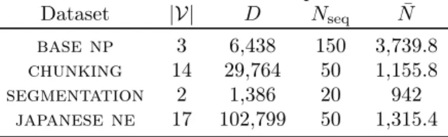
Table 1: Datasets used in our experiments. For each dataset we see the number of categories (or vocabulary |V|), the number of features (D), the number of training sequences (Nseq), and the average (across folds) number of training words (N¯). All
numbers refer to the small-scale experiments.
Dataset |V| D Nseq N¯
base np 3 6,438 150 3,739.8
chunking 14 29,764 50 1,155.8
segmentation 2 1,386 20 942
japanese ne 17 102,799 50 1,315.4
2007) that only takes in consideration the local inter-actions within a single factor between the variables in our model. We emphasize that this change did not require any modification to our inference engine and we simply used this pseudo-likelihood as a drop-in replacement for the exact likelihood.
6
EXPERIMENTS
In this section we evaluate our approach using small-scale experiments on the benchmarks used by Bratières et al. (2015), which target several standard nlpproblems and are summarized in Table 1. These include noun phrase identification (base np); chunk-ing, i.e. shallow parsing labels sentence constituents (chunking); identification of word segments in
se-quences of Chinese ideograms (segmentation); and Japanese named entity recognition (japanese ne). We also consider larger-scale experiments on base np and chunking, which have significantly more training data available.
6.1 Small-scale experiments
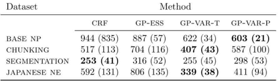
When comparing the error rates on Table 2 we see that our approach is on par with competitive bench-marks which, unlike our method, exploit the structure of the likelihood. More importantly, when analyzing the test likelihoods on Table 3 we see that our method with true likelihood (gp-var-t) is significantly better thancrf for all benchmarks exceptsegmentation, where it has a similar performance. Finally, the log-likelihood results ofgp-ess (Bratières et al., 2015) are also consistently worse than ours, owing largely to the higher computational cost of sampling. 6.2 Larger-scale experiments
Here we evaluate our approach on base np and chunkingusingNseq= 500training sequences and
the remaining (323) sequences for testing, with a five-fold cross-validation setting. This amounts to roughly11,611words on average. We compare with crf, as this was the best baseline in our previous experiments. We also note that that the original gp-essmethod is completely impractical in this setting. Onbase np, our method has a lower average test log-likelihood (1265.52vs. 1355.63) but a higher error rate (5.15%vs4.50%) thancrf. This reinforces our previous message that our method can provide better predictive probabilities than its competitors. How-ever, our results onchunking,2511.48vs1862.96 for test log-likelihoods and8.60%vs7.20%for error rates, indicate that our method lags behindcrfon this dataset. We attribute this result tochunking having a much higher dimensionality thanbase np, which is a more critical issue with large datasets.
7
RELATED WORK
Recent advances in sparsegpmodels for regression (Titsias, 2009; Hensman et al., 2013) have allowed the applicability of such models to very large datasets, opening opportunities for the extension of these ideas to classification and to problems with generic i.i.d like-lihoods (Hensman et al., 2015a; Nguyen and Bonilla, 2014; Dezfouli and Bonilla, 2015; Hensman et al., 2015b). However, none of these approaches is ac-tually applicable to structured prediction problems, which inherently deal with non-i.i.d likelihoods. Twin Gaussian processes (Bo and Sminchisescu, 2010) address structured continuous-output problems by forcing input kernels to be similar to output kernels. In contrast, here we deal with the harder problem of structureddiscrete-output problems, where one usu-ally requires computing expensive likelihoods during training. The structured continuous-output prob-lem is somewhat related to the area of multi-output regression withgps for which, unlike discrete struc-tured prediction withgps, the literature is relatively mature (Álvarez et al., 2010; Álvarez and Lawrence, 2011, 2009; Bonilla et al., 2008).
The original structured Gaussian process model, (gpstruct, Bratières et al., 2015) uses Markov Chain Monte Carlo (mcmc) sampling as the infer-ence method and is not equipped with sparsifica-tion techniques that are crucial for scaling to large data. Bratières et al. (2014) have explored a dis-tributed version ofgpstruct based on the pseudo-likelihood approximation (Besag, 1975) where several weak learners are trained on subsets ofgpstruct’s latent variables and bootstrap data. However, within 7
Table 2: Mean error rates and standard deviations in brackets on small-scale experiments using 5-fold cross-validation. The average number of observed words (N¯) on these problems range from 942 to 3740. svm corresponds to structured support vector machines;crf to conditional random fields;gp-esscorresponds to gpstructwithess for inference (Bratières et al., 2015);gp-var-tcorresponds to our method with true likelihood; andgp-var-pcorresponds to our our method with piecewise pseudo-likelihood.
Dataset Method
svm crf gp-ess gp-var-t gp-var-p
base np 5.9 (0.4) 5.3 (0.5) 5.1 (0.4) 5.6 (0.5) 5.2 (0.3) chunking 9.8 (1.0) 8.5 (1.0) 8.5 (1.0) 9.4 (1.6) 9.0 (1.0) segmentation 16.2 (2.2) 15.4 (1.1) 14.9 (1.8) 14.5 (1.5) 15.3 (2.2) japanese ne 5.6 (0.8) 5.2 (0.7) 5.6 (0.7) 5.4 (0.6) 5.6 (0.6)
Table 3: Negative expected log-likelihoods and standard deviations in brackets on small-scale experiments using 5-fold cross-validation. As before,crfrefers to conditional random fields;gp-essto gpstructwith essfor inference (Bratières et al., 2015);gp-var-tto our method with true likelihood; andgp-var-pto our method with piecewise pseudo-likelihood.
Dataset Method
crf gp-ess gp-var-t gp-var-p base np 944 (835) 887 (57) 622 (34) 603 (21) chunking 517 (113) 704 (116) 407 (43) 587 (100) segmentation 253 (41) 316 (52) 255 (45) 298 (53) japanese ne 592 (131) 806 (135) 339 (38) 411 (94)
each weak learner, inference is still done viamcmc. A variational alternative forgpstructinference (Sri-jith et al., 2014, 2016) is also available. However, it relies on pseudo-likelihood approximations and was only evaluated on small-scale problems. Unlike this work, our approach can deal with both pseudo-likelihoods and generic (linear-chain) structured like-lihoods, and we rely on our sparse approximation procedure and our automated variational inference technique – rather than on bootstrap aggregation – to achieve good performance on larger datasets.
8
CONCLUSION & DISCUSSION
We studied a Bayesian structured prediction model withgppriors and linear-chain likelihoods. We devel-oped an automated variational inference algorithm that is statistically efficient in that only requires ex-pectations over very low-dimensional Gaussians in order to estimate the expected likelihood term in the variational objective. We exploited these types of theoretical insights as well as practical statistical and optimization tricks to make our inference framework scalable and effective. Our model generalizes recent advances incrfs (Koltun, 2011) by allowing general positive definite kernels defining their energyfunc-tions and opens new direcfunc-tions for combining deep learning with structure models (Zheng et al., 2015). As mentioned in the introduction, for general struc-tured prediction problems one may need to set up the configuration of the latent functions (e.g. the unary and pairwise functions in the linear-chain case). Thus, the process of developing an inference procedure for a different structure (e.g. when considering higher-order interactions) requires some human intervention. Nevertheless, when applied to fixed structures our approach is “black box” with respect to the choice of likelihood, inasmuch as different likelihoods can be used without any change to the inference engine. Furthermore, we have already seen in our small-scale experiments a possible way to extend our method to more general structured likelihoods, where the exact likelihood is replaced by a piecewise pseudo-likelihood. Such an approach might be considered for using our framework in models such as grids or skip-chains, for which the evaluation of the true structured likelihood would be intractable.
Overall, we believe our approach is a fundamental step to developing automated inference methods for general structured prediction problems.
References
Mauricio Álvarez and Neil D Lawrence. Sparse convolved Gaussian processes for multi-output regression. In NIPS, pages 57–64. 2009.
Mauricio A Álvarez and Neil D Lawrence. Computa-tionally efficient convolved multiple output Gaussian processes. JMLR, 12(5):1459–1500, 2011.
Mauricio A. Álvarez, David Luengo, Michalis K. Titsias, and Neil D. Lawrence. Efficient multioutput Gaussian processes through variational inducing kernels. In AISTATS, 2010.
Julian Besag. Statistical analysis of non-lattice data. Journal of the Royal Statistical Society. Series D (The Statistician), 24:179–195, 1975.
David M Blei, Michael I Jordan, and John W Paisley. Variational Bayesian inference with stochastic search. InProceedings of the 29th International Conference on Machine Learning (ICML-12), pages 1367–1374, 2012. Liefeng Bo and Cristian Sminchisescu. Twin Gaussian
processes for structured prediction.International Jour-nal of Computer Vision, 87(1-2):28–52, 2010.
Edwin V. Bonilla, Kian Ming A. Chai, and Christopher K. I. Williams. Multi-task Gaussian process prediction. InNIPS. 2008.
Sébastien Bratières, Novi Quadrianto, Sebastian Nowozin, and Zoubin Ghahramani. Scalable Gaussian process structured prediction for grid factor graph applications. InICML, 2014.
Sébastien Bratières, Novi Quadrianto, and Zoubin Ghahramani. GPstruct: Bayesian structured predic-tion using Gaussian processes.IEEE TPAMI, 37:1514– 1520, 2015.
Amir Dezfouli and Edwin V Bonilla. Scalable inference for Gaussian process models with black-box likelihoods. InNIPS. 2015.
Noah D. Goodman, Vikash K. Mansinghka, Daniel M. Roy, Keith Bonawitz, and Joshua B. Tenenbaum. Church: A language for generative models. InUAI, 2008.
James Hensman, Nicolo Fusi, and Neil D Lawrence. Gaus-sian processes for big data. InUAI, 2013.
James Hensman, Alexander Matthews, and Zoubin Ghahramani. Scalable variational Gaussian process classification. InAISTATS, 2015a.
James Hensman, Alexander G Matthews, Maurizio Filip-pone, and Zoubin Ghahramani. MCMC for variation-ally sparse Gaussian processes. InNIPS. 2015b. Matthew D. Hoffman and Andrew Gelman. The
no-u-turn sampler: adaptively setting path lengths in Hamiltonian Monte Carlo. JMLR, 15(1):1593–1623, 2014.
Michael I Jordan, Zoubin Ghahramani, Tommi S Jaakkola, and Lawrence K Saul. An introduction to variational methods for graphical models. Springer, 1998.
Vladlen Koltun. Efficient inference in fully connected CRFs with Gaussian edge potentials. InNIPS, 2011.
John D. Lafferty, Andrew McCallum, and Fernando C. N. Pereira. Conditional random fields: Probabilistic mod-els for segmenting and labeling sequence data. In ICML, 2001.
Iain Murray, Ryan Prescott Adams, and David J.C. MacKay. Elliptical slice sampling. InAISTATS, 2010. Trung V. Nguyen and Edwin V. Bonilla. Automated
variational inference for Gaussian process models. In NIPS. 2014.
Manfred Opper and Cédric Archambeau. The variational Gaussian approximation revisited.Neural computation, 21(3):786–792, 2009.
Joaquin Quiñonero-Candela and Carl Edward Rasmussen. A unifying view of sparse approximate Gaussian pro-cess regression. JMLR, 6:1939–1959, 2005.
Rajesh Ranganath, Sean Gerrish, and David M. Blei. Black box variational inference. In AISTATS, 2014. P. K. Srijith, P. Balamurugan, and Shirish Shevade.
Effi-cient variational inference for Gaussian process struc-tured prediction. InNIPS Workshop on Advances in Variational Inference, 2014.
P.K. Srijith, P. Balamurugan, and Shirish Shevade. Gaus-sian process pseudo-likelihood models for sequence labeling. InECML-PKDD 2016, 2016.
Charles Sutton and Andrew McCallum. Piecewise pseu-dolikelihood for efficient training of conditional random fields. InICML, 2007.
Ben Taskar, Carlos Guestrin, and Daphne Koller. Max-margin Markov networks. InNIPS. 2004.
Michalis Titsias. Variational learning of inducing vari-ables in sparse Gaussian processes. InAISTATS, 2009. Ioannis Tsochantaridis, Thorsten Joachims, Thomas Hof-mann, and Yasemin Altun. Large margin methods for structured and interdependent output variables. JMLR, 6:1453–1484, December 2005.
Shuai Zheng, Sadeep Jayasumana, Bernardino Romera-Paredes, Vibhav Vineet, Zhizhong Su, Dalong Du, Chang Huang, and Philip HS Torr. Conditional random fields as recurrent neural networks. In Proceedings of the IEEE International Conference on Computer Vision, pages 1529–1537, 2015.