Incentive Effects of Fiscal Equalization: Has Russian Style Improved?

(1)

Deutsches Institut für Wirtschaftsforschung

www.diw.de

Lev Freinkman • Konstantin A. Kholodilin •

Ulrich Thießen

Berlin, July 2009

Incentive Effects of Fiscal Equalization:

Has Russian Style Improved?

912

(2)

Opinions expressed in this paper are those of the author and do not necessarily reflect views of the institute.

IMPRESSUM

DIW Berlin

German Institute for Economic Research Mohrenstr. 58

10117 Berlin

Tel. +49 (30) 897 89-0 Fax +49 (30) 897 89-200 http://www.diw.de

ISSN print edition 1433-0210 ISSN electronic edition 1619-4535

Available for free downloading from the DIW Berlin website.

Discussion Papers of DIW Berlin are indexed in RePEc and SSRN. Papers can be downloaded free of charge from the following websites:

http://www.diw.de/english/products/publications/discussion_papers/27539.html http://ideas.repec.org/s/diw/diwwpp.html

(3)

Incentive Eﬀects of Fiscal Equalization:

Has Russian Style Improved?

Lev Freinkman

∗

Konstantin A. Kholodilin

∗∗

Ulrich Thießen

§

July 28, 2009

Abstract

The effects of inter-government fiscal arrangements on variation in re-gional economic growth are analyzed for Russia, a country with large cross-regional differences and considerable fiscal redistribution. More-over, fiscal reforms implemented in the first half of 2000s, which fol-lowed to some extent scientific advice, make analysis of this case par-ticularly interesting. We observe that post-reform fiscal redistribution became more rational and this resulted in fewer incentive distortions. We found no negative association between federal transfers and re-gional growth. Furthermore, there are no major differences between donor and recipient regions in the way how inter-governmental fiscal arrangements influence regional growth. Overall, fiscal policy vari-ables have become less important growth determinants than it was the case in the 1990s. Still further reforms in federalism arrangements would be desirable.

Keywords: Fiscal equalization; inter-governmental ﬁnance reform; Russian regions; extreme bounds analysis.

JEL classiﬁcation: C21; E62; H77; R11

∗_{Academy of National Economy, Moscow, Russia and World Bank, Washington, DC,}

USA,e-mail: [email protected]

∗∗_DIW _Berlin, _{Mohrenstraße} _58, ₁₀₁₁₇ _Berlin, _Germany, _e-mail:

[email protected]

(4)

List of Tables

1 Variables used in the study. . . 19

2 Descriptive statistics of the ﬁscal variables by subperiods . . . 22

3 Correlation between retention rates, per-capita transfers, and per-capita GRP in levels and in growth rates, cross-section averaged over 1998-2006 . . . 23

4 EBA cross-section OLS estimation, 1999-2006 . . . 24

7 EBA cross-section OLS estimation by donors and recipients, 1999-2001 . . . 27

8 EBA cross-section OLS estimation by donors and recipients, 2002-2006 . . . 28

9 EBA cross-section 2SLS estimation by donors and recipients, 1999-2001 . . . 29

10 EBA cross-section 2SLS estimation by donors and recipients, 2002-2006 . . . 30

List of Figures

1 Retention rate versus per-capita GRP, average over 1998-2006 31 2 Eﬀectiveness of ﬁscal equalization, average over 1998-2006 . . 32

(6)

1 Introduction

The purpose of the paper is to analyze incentive effects of the modern fiscal equalization system in Russia, which has emerged after the implementation of inter-governmental fiscal reforms in the early 2000s. Russia is an ideal country to study these effects because its large size, major regional income and growth disparities, and high concentration of natural resource wealth constitute the major reasons to justify the existence of a relatively large inter-governmental equalization system.

The paper is structured as follows: Section 2 discusses briefly the lit-erature of incentive effects of fiscal equalization. Section 3 summarizes the relevant Russian reforms. Section 4 explains our approach of using extreme bounds analysis to examine the incentive effects and presents the main re-sults. Finally, section 5 concludes.

2 Literature on incentive eﬀects of ﬁscal

equal-ization

The theoretical case for fiscal equalization is well established and largely undisputed (e.g.,Boadway and Keen(1996),Bordignon et al.(2001),Dahlby and Wilson (2003)). And the theory is continuously extended by consider-ing additional and important externalities between regions. For instance, recently the possibility of mitigating harmful tax competition through fiscal equalization was demonstrated (Köthenbürger(2002),Grazzini and Petretto

(2005), Bucovetsky and Smart (2006)). However, it is also true that fiscal equalization may have unforeseen detrimental effects, which should be care-fully studied because society has a right to know whether the benefits of having a fiscal equalization system are larger than its costs.

Despite a rapidly growing literature on fiscal federalism and its popu-lar subtopic of fiscal decentralization, explicit empirical analysis of incentive effects of fiscal equalization appears to be still in its infancy:

∙ In one of the first publications on these effects, Smart and Bird(1997) showed for the Canadian fiscal equalization system that federal trans-fers tended to be associated with higher tax rates in relatively poor regions. Higher tax rates negatively affect economic performance of

(7)

the poor regions since they discourage investment. Therefore, the fed-eral budget provided transfers in order to compensate for these losses.

∙ Building on this work and on Bordignon et al. (2001), Baretti et al.

(2002) performed a pioneering theoretical and empirical analysis for Germany. This is a particularly interesting case because both donor and recipient regions faced very high marginal “tax rates” (well above 90%) on their regional revenues or, in other words, very low retention rates, which is the notation used in this paper. Plausibly, the authors found that these high marginal tax rates had statistically significant negative effects on regional performance indicators, such as economic growth and tax revenues. Eggert et al. (2007) found that the regional transfers provided by the EU structural funds also had significant neg-ative effects on long-term real economic growth in Germany, despite the fact that they promoted regional convergence.

∙ For Spain,Balaguer-Coll et al.(2004) studied the efficiency of local pub-lic expenditures using a non-parametric estimation. They distinguished between allocative, technical, and cost inefficiency. It was shown that the inefficiencies were primarily of the allocative type, i.e., a suboptimal structure of factors is chosen. Thus, a “simple” restructuring of spend-ing could increase efficiency of public expenditure. Although this is not an explicit analysis of incentive effects, it confirms the importance of incentives provided to subnational governments.

∙ For 19 high-income OECD countries,Feld and Dede (2005) found that tax autonomy of subnational governments does not appear to have a ro-bust eﬀect on economic growth. But they found a negative association between the communal share in the total tax revenues and economic growth. This suggests that a clear deﬁnition of responsibilities regard-ing decisions on taxes and spendregard-ing is a prerequisite for revenue and spending autonomy to result in a growth-promoting environment.

∙ Regarding transition countries, several of the studies concern Russia and, to the best of our knowledge, there is only one study on China and one on Ukraine. The China study concentrates on incentives for local governments to develop their own revenue base and the effects of this development (Jin et al. (2004)). It finds that there are substan-tial regional differences in these incentives and that stronger revenue

(8)

incentives tend to be beneficial for economic development. The study on Ukraine argues that the moderate scale of regional revenue redistri-bution can well explain why the country’s equalization system did not appear to have adverse growth effects (Thießen (2004)). Surprisingly, significant positive effects on regional economic per-capita growth of the fiscal equalization system were found for both donor and recipient regions. This is the exact opposite of the finding for Germany, but it is plausible, because retention rates and the degree of fiscal redistribution are very different in both countries.

∙ For Russia, there are several explicit studies of incentive effects but they use the data for the period of the 1990s, i.e., before the new round of Russian inter-governmental fiscal reforms in the early 2000s became ef-fective. They all agree that the former system had substantial deficien-cies mainly because of its non-transparency,ad hoc decisions regarding transfers, unfunded expenditure mandates, and arbitrary distribution of revenues. Together with the unsolved task of avoiding disincen-tives caused by Russia’s natural resource wealth, these contributed to short-term horizons of decision making by regional government, poor efficiency of public goods provision, and economic growth losses ( Zhu-ravskaya(2000),Alexeev and Kurlyandskaya(2003),Popov(2004), De-sai et al. (2005), Thießen (2006), Freinkman and Plekhanov (2009)). Of these contributions our following analysis is closest to that ofDesai et al.(2005) in examining the effects of fiscal equalization on per-capita GDP growth, because we use the same main indicators of the equal-ization system, namely the retention rate each region faces and inter-governmental transfers from the federal center to regions. The main difference is that we employ extreme bounds analysis (EBA): Since the relationships between regional growth, the fiscal equalization system, and other potential influences are still very complex, we need to con-sider many variables and this raises the question of sensitivity of the results.

∙ Potential growth determinants in Russian regions were also analyzed in Ahrend (2008) using extreme bounds analysis, but he did not con-sider eﬀects of ﬁscal equalization. In addition, Ahrend is interested in the whole post-Soviet period since 1993, i.e., including the downturn period, whereas we examine only the growth period since 1999, which

(9)

is much more homogeneous and also mandated by data limitations. According toAhrend (2008), after 1998, regional growth in Russia has been largely determined by the hydrocarbon wealth and advantageous geographical location. More reform-oriented policies, as well as better regional leadership are also found to play signiﬁcant part.

∙ In a recent study,Zubarevich(2009) has identiﬁed the following key fac-tors that are commonly seen as central to variation in regional growth rates in Russia since 1999: 1) economy of scale that provided advan-tages to regions that host the country’s largest industrial centers; 2) availability of extracting industries, in particular oil and gas; and 3) coastal location, especially in the European part of Russia.

Finally, perhaps also influenced by these analyses, many industrial coun-tries have recently carried out reforms of their fiscal equalization systems. Although the reforms differed substantially in their details, they showed two common features: They have intended to strengthen the subnational govern-ments’ incentives and reduce the scale of horizontal redistribution relative to GDP (e.g., Arachi and Zanardi (2004) for Italy and Blöchliger et al. (2007) for an overview of OECD countries).

3 Russia’s inter-governmental ﬁscal reforms

since 2001

The Russian inter-governmental ﬁnance reforms in the early 2000s have been described in detail, among others, in Kadochnikov et al. (2008), Martinez-Vazquez et al. (2006), as well as Martinez-Vazquez and Timofeev (2008),

Thornton and Nagy (2006), and Hanson (2006). Therefore, it may suﬃce here to summarize major points of interest.

The reforms included a strengthening of the federal revenues at the ex-pense of the initial retention in the regions of locally-raised tax revenue and thus were accompanied by an increase in transfers from the federal center to regions1_{. But at the same time there was a clariﬁcation of the division of}

pow-ers between levels of government both with regard to taxation and spending, 1

From 2000 to 2002 transfers from the federal Russian budget to the regions increased from about 1.5% to 3% of GDP. Since then it ﬂuctuated between 2.2% and 2.8% of GDP.

(10)

which to a large degree followed scientific advice. For instance, tax sharing was substantially reduced. Revenues from taxes on natural resource wealth were given almost entirely to the federal government. Subnational govern-ments were given exclusively the revenues from personal income taxes, several important excises, and from inheritance, property and small business taxes. In 2008, federal government revenues equaled about 22% of GDP, while subnational government revenues attained about 15% of GDP before trans-fers (computed using the data on the execution of government budget bor-rowed from the database of the State Treasury of Russiahttp://www.roskazna. ru/reports/cb.html). Although these subnational government revenues are not sufficient for adequate financing of subnational expenditure responsibil-ities, there is now a responsibility of the federal government to finance all delegated expenditures via transfers, at least on paper. Hence, unfunded ex-penditure mandates were largely eliminated, while there is more transparency now regarding the allocation of expenditure responsibilities.

Also, Russia introduced other inter-governmental ﬁscal reforms in the be-ginning of the 2000s, notably the tax reforms with a reduction of the number of taxes and drastic cuts in tax rates, which made tax administration sim-pler, increased acceptance of the tax system, and promoted tax compliance (Gorodnichenko et al. (2008)). This contributed to the upsurge of income tax revenues relative to GDP, which to a large extent accrue to subnational governments.

Reforms were also introduced regarding the inter-governmental transfer system: The most important instrument of fiscal equalization, the “Fund for Financial Support of the Regions” (FFSR) was reformed. This fund is sup-posed to reduce horizontal per-capita revenue differences and together with other formula-based funds administers about 70% of all federal financial as-sistance to regions. FFSR transfers are strictly based on formulae and most recently a three-year plan for transfer allocations was introduced. Also the second most important fund for financial assistance to regions, the “Com-pensation Fund” (CF), which finances federally mandated expenditures, is based on formulae. The formulae are very advanced and complicated because they intend to consider many aspects of the “need” of regions2_.

Although there are still essential weaknesses in Russia’s intergovernmen-2

The methodology of computing the transfers, that are carried out through FFSR and CF, can be found (in Russian) on the webpage of the Ministry of Finance of Russia

(11)

tal ﬁscal arrangements, and the system is still subject to much criticism, the overall direction of these reforms was towards an improvement in trans-parency, accountability, impartiality, and thus possibly it brought about bet-ter incentives for subnational governments to improve the eﬃciency of public goods delivery. This provides the impetus for our analysis.

However, it has to be noted that another reform was introduced in 2005, which made appointment of regional governors largely dependent upon Rus-sia’s president. Direct elections of governors by the regional electorate were abolished. Regional parliaments now vote on governor candidates upon the recommendation of the president. The president has the right to dissolve regional legislature if his candidates are repeatedly rejected. This leads, of course, to a substantial detachment of governors from their regional elec-torate. But the theory of fiscal federalism is built on the assumption that the regional governments are accountable to their electorate and follow, in principle, their will. Hence, this setting may distort the incentive structure of regional governments, i.e., its impact is in the direction that is opposite to the one of fiscal reforms. Since we do not know the relative strength of these two effects, we have to emphasize this institutional anomaly as a potentially important qualification of our analysis.

4 Econometric estimation

4.1 Extreme bounds analysis

There is a vast econometric literature exploring the impact of different eco-nomic, social, institutional, and political factors on economic growth. In many cases, the regressions include only small number of potential combi-nations of explanatory variables. Hence, they may ignore some important factors strongly correlated with growth. Therefore, it is virtually impossible to judge about the robustness of such results, since they may turn insignifi-cant (fully or partially) under alternative specifications.

In order to check the robustness of parameter estimates for a variable of interest, the so-called extreme bounds analysis can be used. This approach was suggested by Leamer (1983) and basically implies trying all possible combinations of variables in order to obtain the distribution of the param-eter estimates of interest under all alternative speciﬁcations. The extreme upper (lower) bound is deﬁned as the maximum (minimum) of all thus

(12)

ob-tained parameter estimates plus (minus) two standard errors. The parameter estimate is judged to be robust if both extreme bounds have the same sign.

However, as Sala-i-Martin (1997a,b) has claimed, this approach is too restrictive for any variable to pass the EBA test. The reason is that, if the distribution of parameter estimates has some positive and some negative support, then one inevitably finds at least one regression, for which the esti-mated coefficient changes the sign if enough regressions are run. Therefore, he suggests using as a test of robustness the cumulative density function es-timated at zero, 𝐶𝐷𝐹(0). In fact, the larger of the areas under the density function above or below zero (i.e., regardless of whether this is 𝐶𝐷𝐹(0) or 1−𝐶𝐷𝐹(0)) is denoted as 𝐶𝐷𝐹(0), which therefore varies between 0.5 and 1. According to this test, the estimated parameter is said to be robust, or significant, if 𝐶𝐷𝐹(0) > 0.95. This test is equivalent to checking whether the 90% interval (between 5-th percentile and 95-th percentile) in the distri-bution of a parameter includes zero.

To the best of our knowledge, there is only one paper applying EBA to the analysis of economic growth in Russian regions, namely —Ahrend(2008). It examines a wide range of factors that possibly affect growth, however, does not consider the effects of inter-governmental fiscal arrangements.

A typical regression equation for EBA is deﬁned as:

𝑌 =𝑆𝑉 𝛼+𝛽𝑉 𝐼+𝐴𝑉 𝛾 +𝑢 (1) where 𝑌 is the dependent variable; 𝑆𝑉 is the matrix of core “standard” ex-planatory variables, which are commonly included in the growth regressions; 𝑉 𝐼 is the variable of interest; 𝐴𝑉 is the matrix of several (usually three) additional explanatory variables, and 𝑢is an error term.

As dependent variable the average annual growth rate of real Gross Re-gional Product (GRP) over the period 1998-2006 was taken.

There are two groups of fiscal variables of interest. The first group in-cludes the retention rate (RR) of the regions, reflecting the share of locally collected taxes retained by the regional budgets. Three different measures of RR are used. First, RR has been computed based on total regional revenues, 𝑅𝑅𝑎; second, on the revenues from all the main taxes (such as profit tax, in-come tax, VAT, excises, various mineral resources taxes, and land tax), 𝑅𝑅𝑏; and, third, on the revenues from the main taxes excluding VAT and mineral resources taxes, 𝑅𝑅𝑐. The VAT and most resource taxes are the key source of federal revenues, which since 2001 have not been shared with subnational

(13)

governments. Thus, the collection and sharing of the latter taxes has the least impact on incentives of regional governments.

Each measure of retention ratio is calculated as: 𝑅𝑅= 𝑅𝑒𝑣𝑒𝑛𝑢𝑒𝑅

𝑅𝑒𝑣𝑒𝑛𝑢𝑒𝑇

(2) where 𝑅𝑒𝑣𝑒𝑛𝑢𝑒𝑇 is the total revenue collected at the regional level before being distributed between the revenue going to the federal budget,𝑅𝑒𝑣𝑒𝑛𝑢𝑒𝐹, and that remaining at the regional level, 𝑅𝑒𝑣𝑒𝑛𝑢𝑒𝑅.

The second group of ﬁscal variables is represented by the transfer ratios (𝑇 𝑅), reﬂecting regional dependence on federal transfers. Again, as in the case of retention rate, there are three alternative measures of transfer ratio depending on the revenue base: 𝑇 𝑅𝑎, 𝑇 𝑅𝑏, and 𝑇 𝑅𝑐. Each measure of transfer ratio is calculated as:

𝑇 𝑅= 𝑇 𝑟𝑎𝑛𝑠𝑓 𝑒𝑟𝐹2𝑅 𝑅𝑒𝑣𝑒𝑛𝑢𝑒𝑅

(3) where 𝑇 𝑟𝑎𝑛𝑠𝑓 𝑒𝑟𝐹2𝑅 is the total federal transfers to regions, which are not of reimbursable nature, i.e., excluding federal budget loans granted to the regions. The ratio is deﬁned in the interval [0,+∞), since the transfers in some cases by far and large exceed3 _{the revenues remaining at the regional}

level after all the federal revenues are transmitted to the federal budget. On average in 1999-2006, Russian regions retained between 60% and 80% (depending on the definition of retention rate) of taxes they collected, and this rate has either remained unchanged (in case of 𝑅𝑅𝑎) or increased by about 10% (in case of 𝑅𝑅𝑏 and 𝑅𝑅𝑐) over the period. As Table 2 shows, the variation (as measured by coefficient of variation, or CV) of both re-tention rates and transfer ratios across regions has decreased in the second subperiod, 2002-2006, compared to the first subperiod, 1999-2002. This is mainly due to the fact that the minimum retention rates and transfer ratios have substantially increased. In case of transfer ratios, a reduction in the maximum values has also contributed to the decline in CV, too. The decline in variation of these fiscal variables suggest, in our view, that the system of regional fiscal redistribution in Russia has been evolving in the direction of the system of inter-governmental arrangements that is based on the

univer-3

This is, for example, the case of some Caucasus republics as well as of Republic of Altai.

(14)

sal legal and regulatory framework, with fewer exemptions and special deals between the center and individual regions.

It can be assumed that the effects of fiscal federalism can be different depending on whether the region is net donor or recipient of the federal budget resources. The donor/recipient regions can be distinguished based on the difference between the revenues going to the federal budget and the transfers returning to the regional level, 𝑅𝐹−𝑇𝐹2𝑅. Thus, if𝑅𝐹−𝑇𝐹2𝑅 >0, the region is said to be a donor, otherwise it is denoted as a recipient. In other words, a donor (recipient) is a region that gives to the federal budget more (less) than what it obtains from the federal budget as a transfer4_{. Given that}

we consider three diﬀerent measures of revenues, there are also three options for the donor/recipient dummy. When all the revenues are accounted for, one can identify 49 donor regions out of the total of 77 regions. When only main tax revenues and main tax revenues excluding natural resource taxes and VAT are considered, the number of donor regions is reduced to 45 and 21, respectively.

A modiﬁed version of the original equation (1), where the regions are split into donors and recipients, was estimated:

𝑌 =𝑆𝑉 𝛼+𝛽1𝐼𝑑𝑜𝑛𝑜𝑟/𝑟𝑒𝑐𝑖𝑝𝑖𝑒𝑛𝑡𝑉 𝐼+𝛽2(1−𝐼𝑑𝑜𝑛𝑜𝑟/𝑟𝑒𝑐𝑖𝑝𝑖𝑒𝑛𝑡)𝑉 𝐼+𝐴𝑉 𝛾+𝑢 (4) where 𝐼𝑑𝑜𝑛𝑜𝑟/𝑟𝑒𝑐𝑖𝑝𝑖𝑒𝑛𝑡 is a dummy variable equal to one, when the region is donor, and zero, when the region is recipient.

In the seminal paper on cross-country growth regressions by Levine and Renelt(1992), the matrix𝑆𝑉 includes four variables: initial GDP per capita, investment share of GDP, as a proxy for physical capital, as well as the average annual population growth rate and the secondary school enrollment rate as proxies for human capital.

In his recent paper on the determinants of growth in Russian regions,

Ahrend (2008) uses only two standard variables: initial GRP per capita and secondary school enrollment rate. He claims that the investment data for Russian regions are not reliable at all and drops the population variable without commenting.

In this paper, we have decided to replace the secondary school enrollment rate with the university enrollment rate (share of the university students in

4

Alone the fact that a region obtains transfers from the federal budget cannot serve as an indication that this region is donor. In fact, almost all regions get transfers. The few exceptions are Bashkortostan in 1998 as well as Moscow in 1999 and 2000.

(15)

total regional population averaged over 2000-2006), because secondary edu-cation in Russia is compulsory. As a result, the former variable is not very informative and displays no noticeable variation — see Table1. By contrast, the university enrollment rate varies a lot and may serve as a better proxy for human capital diﬀerences across the regions5_{. In addition, the population}

growth variable is included in our𝑆𝑉-variables list, for, given very low natu-ral population growth in Russia, its regional dynamics reflects the migratory flows of the qualified labor force. Many poor regions, especially those to the east of Ural mountains, are characterized by a substantial outflow of the la-bor force, which negatively affects their production potential, whereas richer regions in the European part of Russia benefit from the inflow of the qualified workers. Finally, as a third standard variable, we used the per-capita GRP in 1998 corrected for the purchasing power parity (PPP) factor of Granberg and Zaitseva (2002) that allows accounting for the existing large price level differences among Russian regions. To sum up, our set of 𝑆𝑉-variables in-cludes three variables: real per-capita GRP in 1998, university enrollment rate, and annual average rate of population growth.

Following the tradition of the EBA literature, the number of additional variables included in each regression was set to three. This number allows keeping the number of regressions with diﬀerent combinations of explanatory variables manageable. Thus, given that the total pool of additional variables in our case contains 35 series, there would be 6,545 combinations with three 𝐴𝑉-variables, 52,360 with four variables, 324,632 with ﬁve𝐴𝑉-variables, and so on.

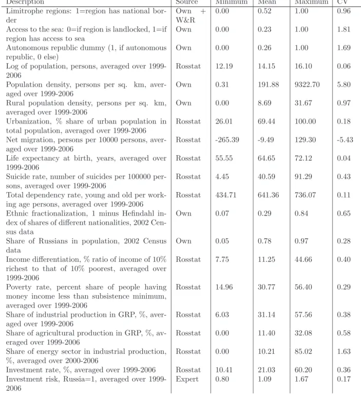
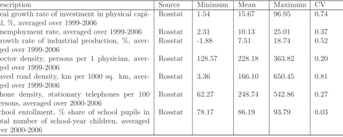
All the variables used in these estimations are listed in Table 1. The table reports the sources of data as well as some descriptive statistics, such as minimum, mean, maximum, and coeﬃcient of variation.

4.2 Econometric results

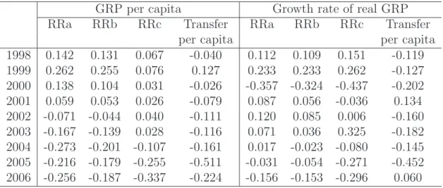
Before we turn to the estimation results, let us examine simple linear cor-relations between the variables of interest, which are reported in Table 3. The correlations between retention rates and per-capita GRP levels are de-clining almost continuously during the whole sample period and turn from

5

Another option to proxy regional human capital is by using the share of employees having higher education in total regional employment. However, in that case, the esti-mation results are very similar to those obtained with the university enrollment rate. In order to save space these results are not reported here but are available on request.

(16)

positive to negative around 2002-2003, that is, in the years immediately af-ter Russia’s inaf-ter-governmental finance reforms were implemented. Thus, tax sharing arrangements became progressive after 2002, since the richer regions tend to have lower retention rates and pay more taxes to the common fed-eral pool of revenues. This may be considered to be a positive effect of the inter-governmental fiscal reforms. These correlations in Table 3 may even underestimate the degree of negative association between the retention rate and per-capita GRP due to the presence of several outliers, notably Tiumen region and Moscow city, as shown in Figure 1 displaying 𝑅𝑅𝑏 versus GRP per capita.

The correlations between per-capita transfers and per-capita GRP levels are also declining over time, although they were always negative. It im-plies that the transfers are increasingly transmitted to the regions that are relatively poor and have a greater need in federal support.

The correlation between retention rates and the annual growth rate of real GRP is rather low and shows no clear trend, although in the last 2-3 years it has been negative. Negative correlation between retention and growth can imply two things. Either higher retention is associated with lower growth, which may mean that leaving to the regions more resources discourages regional governments from stimulating the regional economy, or that richer regions, which have a lower retention rate, grow faster than the poor regions. The latter explanation is not very convincing. It is true that no signiﬁcant convergence between Russian regions has been observed in 1998-2006, but there was no divergence either, since both rich and poor regions grew on average at the same rate during the period, as shown in Kholodilin et al. (2009).

With respect to the ﬁrst potential explanation, our sense is that there is no casualty link here, i.e., higher retention rates do not undermine regional incentives for growth. It is more likely that some regions are obtaining higher retention rates as a compensation for their peculiar local disadvantages (such as remoteness and other geographic constraints) that dampen their longer term growth perspectives. However, more analysis of this interaction may be needed in the future.

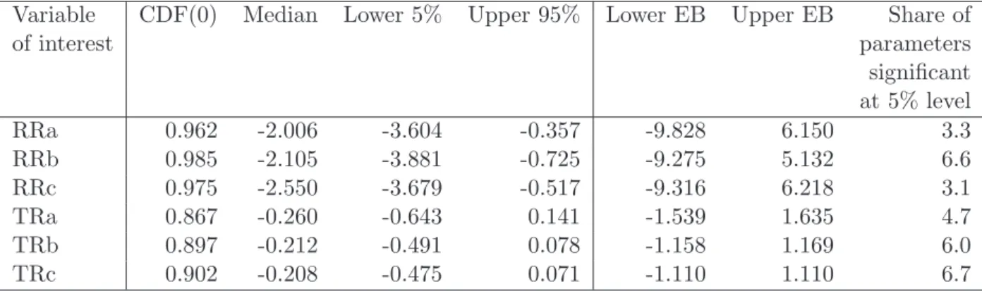
The rest of this section discusses our core regression results. Our investi-gation was undertaken in stages. First, regressions were estimated using the OLS method for the whole period, 1999-2006, without splitting the sample into donor and recipient regions. The estimation results of the models cor-responding to equation (1) are reported in Table 4. The ﬁrst four columns

(17)

contain the measures introduced in Sala-i-Martin (1997a,b), while the last three columns are those due to Leamer(1983). From Table 4 it can be seen that, according to Leamer’s EBA test, all ﬁscal variables are fragile, for the lower and upper extreme bounds have opposite signs. At the same time, according to the Sala-i-Martin measures, all retention variables are robust (since their 𝐶𝐷𝐹(0) exceeds 0.95), while transfer variables remain fragile (𝐶𝐷𝐹(0) < 0.95). The median coeﬃcient estimates of the retention vari-ables have a negative sign implying that an increase of retention rates is associated with slower regional growth.

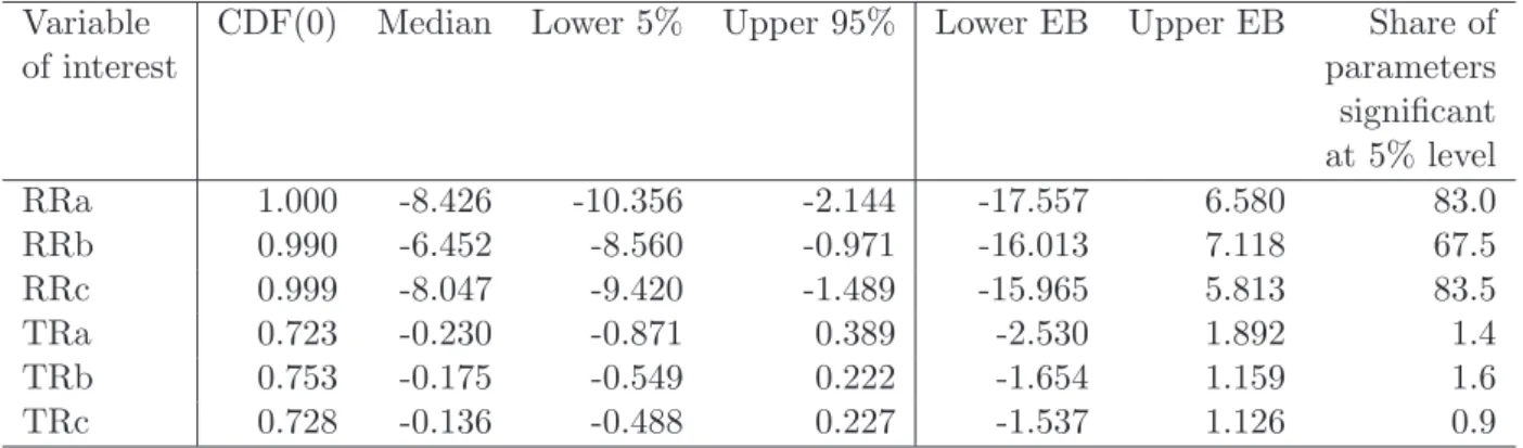
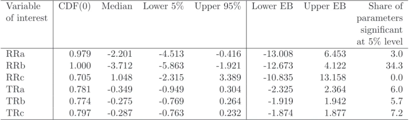
Second, the whole sample was divided into two sub-samples roughly corre-sponding to the pre-reform (1999-2001) and post-reform (2002-2006) periods. The corresponding estimation results are reported in Tables 5 and 6. It can be seen from these tables that, although all transfer variables remain frag-ile in both sub-periods, at least the two first retention variables are robust across both sub-periods. In addition, the median coefficient estimates of𝑅𝑅 variables are far larger before reform than after it was launched. Thus, the reform of the fiscal equalization system put in action in 2001 seems to weaken the link between the retention rate and regional economic growth.

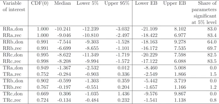
Third, further insights can be gained by splitting regions into two groups: donors and recipients. Tables7and8contain the estimation results obtained by estimating equation (4) for two sub-periods. In 1999-2001, the effect of the retention rate on growth for both donors and recipients was robust. Moreover, they have a similar value for median coefficient estimates. This implies that the impact of the retention rate upon regional growth is similar across both groups of regions. In 2002-2006, only 𝑅𝑅𝑏remains robust, again the median coefficient estimates for donors and recipients are very close. All the transfer ratios in the first sub-period appear to be fragile for both groups of regions. However, in the second sub-period, the impact of transfer ratios of the donor regions prove to be robust and positive, whereas transfer ratios of recipients are still fragile. It can be concluded that after the reform larger transfers to the donor regions started to be positively associated with a stronger growth performance.

Nevertheless, given that transfers are conditioned upon the economic sit-uation in each region, it may well be the case that they are endogenous. Therefore, an additional check is needed to corroborate the robustness of our results obtained for the transfer variables. To do this we re-conducted, at the fourth stage of our analysis, the EBA for transfer variables using the two-stage least squares (2SLS) estimator. As instruments the lagged values of the

(18)

transfer ratios were used. For the first subperiod these are the transfer ratios in 1998, while for the second sub-period — transfer ratios in 2001. The corre-sponding results are reported in Tables9and10. In addition to the standard EBA statistics, these tables contain also 𝑝-values of the Hausman, Sargan, and 𝐽-test as well as a test statistic for the Staiger-Stock’s rule of thumb that allow testing the appropriateness of the selected instruments. If the null hypothesis of Hausman test is rejected, then the corresponding instrumented variable is endogenous. In all the estimated models, the Hausman test is ex-ceeding 0.10 and hence the null hypothesis of endogeneity of the instrumental variable cannot be accepted. The null hypothesis of Sargan (J-)test is that all moment conditions are valid. If the test is rejected, it cannot be determined, which are the invalid moment conditions. In all models, both Sargan test and J-test lead to an acceptance of the validity of instruments. Finally, if Weak (F-statistic of all instruments’ coefficients equal zero estimated at the 1st stage) is lower than 10.27, then instruments are considered as weak, i.e., not correlated with instrumented variable. In all the models we examined, F-statistic is by far and large exceeding the rule-of-thumb critical value of 10.27 and therefore our instruments can be considered as strong. According to these specification tests, the 2SLS models appear to be correctly specified. The results of the 2SLS estimation confirm those obtained using OLS.

The overall important ﬁnding here is the lack of negative association between transfers and regional growth. This is in contrast to the situation in the 1990s, when, as reported by Desai et al. (2005), regional transfer dependence was a signiﬁcant determinant of slower growth.

The robust negative effect of variation in retention on regional growth pat-terns suggests that the inter-governmental finance reforms have been mostly growth encouraging: regions with a higher retention rate showed on average slower growth. This is in a contrast with the results by Desai et al. (2005) obtained for the second half of 1990s, when the retention rate was a positive determinant of regional growth in Russia. This change, in our view, points to a positive shift in inter-governmental fiscal arrangements. We interpret it as a sign that fiscal equalization became much more growth-neutral because higher taxation (lower retention) is not associated any longer with slower growth, and thus, it may suggest that federal government decisions on tax sharing would not affect much decisions of regional governments regarding their development strategy. As a result, regional growth is likely to depend largely on regional fundamentals (labor and resource endowments, geogra-phy), and less on short-term fiscal policy variables related to the politics of

(19)

inter-governmental ﬁscal arrangements. As mentioned above, the fact that the regions with higher retention have slower growth is, in our view, not directly related to inter-governmental ﬁscal arrangements.

Overall, the results for both the retention and transfer variables seem to suggest that the federal inter-governmental ﬁscal policy became much more neutral with respect to regional government incentives to support growth. This is an important positive development.

5 Conclusion

Reforms of inter-government fiscal arrangements introduced in Russia in 2001-2002 have resulted in significant changes and general improvements in incentives of the regional governments. Before the reforms, the relationship between the retention rate and regional economic growth was positive, indi-cating that a higher contribution by regions to the federal budget (lower re-tention rate) was associated with lower growth. Regional taxation hampered the growth incentives. After the reforms, the relationship turned negative, implying that a higher regional tax burden does not result in a growth loss. The correlation between regional per-capita income and the retention rate became negative too. This means that fiscal equalization became more progressive: wealthier regions have been contributing more. Thus, the Rus-sian case is currently in strong contrast to the German one, where very low retention rates appear to discourage regional governments from promoting regional growth. On the other hand, it is similar to the case of Ukraine where, as in Russia, both retention rates and the size of transfers relative to GDP are quite modest and the relationship between the retention rate and regional growth is negative.

We find that inter-governmental fiscal arrangements in Russia became more rational and this resulted in fewer incentive distortions. In particular, we find no negative association between federal transfers and regional growth. And there are no major differences between donor and recipient regions in the way how inter-governmental fiscal arrangements influence regional growth. Still additional reforms in fiscal equalization would be desirable. As shown by Figure2, there is still considerable room for improving the effectiveness of fiscal equalization. There are two problem groups of regions: 1) Those who had higher than average revenues per capita before fiscal equalization and whose position after equalization improved even further (e.g., Magadan and

(20)

Kamchatka). 2) Those who had lower than average revenues before ﬁscal equalization and whose position after equalization further deteriorated (e.g., Cheliabinsk).

The overall quality of fiscal equalization, as measured by the share of regions that after fiscal equalization moved towards the line of neutrality of fiscal equalization (it is equal 100% minus the share of the two aforementioned groups of regions), improved only very slightly over the period of our analysis. In 1998-2000, it was 68.8%, while in 2004-2006 it increased to 70.1 (although in 2001-2003 it fell down to 66.2%). Extending the formula-based approach to a larger share of total transfers could possibly allow overcoming these anomalies and achieving substantial improvements in the quality of fiscal equalization without having to raise the overall size of transfers.

In addition, it needs to be emphasized that the preconditions for ﬁscal federalism to be able to function appear not to be met as long as the re-gional governors are de facto determined by the presidency and less so by the local constituency. A change of this could not only improve meeting the preconditions of ﬁscal federalism but also promote democracy.

References

Ahrend, R. (2008). Understanding Russian regions’ economic performance during periods of decline and growth: An extreme-bound analysis ap-proach. OECD Economics Department Working Papers 644, OECD Eco-nomics Department.

Alexeev, M. and G. Kurlyandskaya (2003). Fiscal federalism and incentives in a Russian region. Journal of Comparative Economics 31(1), 20–33. Arachi, G. and A. Zanardi (2004). Designing intergovernmental ﬁscal

rela-tions: Some insights from the recent Italian reform. Fiscal Studies 25(3), 325–365.

Balaguer-Coll, M. T., D. Prior, and E. Tortosa Ausina (2004). On the de-terminants of local government performance: A two-stage nonparametric approach. European Economic Review 51(2), 425–451.

Baretti, C., B. Huber, and K. Lichtblau (2002). A tax on tax revenue: The incentive eﬀects of equalizing transfers: Evidence from Germany. Interna-tional Tax and Public Finance 9(6), 631–649.

(21)

Bl¨ochliger, H., O. Merk, C. Charbit, and L. Mizell (2007). Fiscal equalization in OECD countries. OECD Working Paper 4, Paris.

Boadway, R. and M. Keen (1996). Eﬃciency and the optimal direction of federal-state transfers. International Tax and Public Finance 3(2), 137– 155.

Bordignon, M., P. Manasse, and G. Tabellini (2001). Optimal regional redistribution under asymmetric information. American Economic Re-view 91(3), 709–723.

Bucovetsky, S. and M. Smart (2006). The eﬃciency consequences of local revenue equalization: Tax competition and tax distortions. Journal of Public Economic Theory 8(1), 119–144.

Dahlby, B. and L. S. Wilson (2003). Vertical ﬁscal externalities in a federa-tion. Journal of Public Economics 87(5-6), 917–930.

Desai, R. M., L. Freinkman, and I. Goldberg (2005). Fiscal federalism in rentier regions: Evidence from Russia. Journal of Comparative Eco-nomics 33(4), 814–834.

Eggert, W., M. von Ehrlich, R. Fenge, and G. König (2007). Konvergenz-und Wachstumseffekte der europäischen Regionalpolitik in Deutschland (Convergence and growth effects of European regional policy in Germany).

Perspektiven der Wirtschaftspolitik 8(2), 130–146.

Feld, L. P. and T. Dede (2005). Fiscal federalism and economic growth: Cross-country evidence for OECD countries. Discussion Paper, Philipps-Universit¨at Marburg.

Freinkman, L. and A. Plekhanov (2009). Fiscal decentralization in rentier regions: Evidence from Russia. World Development 37(2), 503–512. Gorodnichenko, Y., J. Martinez-Vazquez, and K. Sabirianova Peter (2008).

Myth and reality of ﬂat tax reform: Micro estimates of tax evasion response and welfare eﬀects in Russia. NBER Working Papers 13719, National Bureau of Economic Research, Inc.

(22)

Granberg, A. and I. Zaitseva (2002). Производство и использование валового регионального продукта: межрегиональные со-поставления. Статья 2 (Production and use of the gross regional prod-uct: Interregional comparisosn. Second article). Rossijskij ekonomicheskij zhurnal (Russian Economic Journal) 11-12, 48–70.

Grazzini, L. and A. Petretto (2005). Regional fiscal effort and devolution with revenue sharing and equalization. Technical report, SIEP, Università degli Studi di Pavia.

Hanson, P. (2006). Federalism with a Russian face: Regional inequality, administrative capacity and regional budgets in Russia. Economic change and restructuring 39, 191–211.

Jin, H., Y. Qian, and B. Weingast (2004). Regional decentralization and ﬁscal incentives: Federalism, Chinese style. Journal of Public Economics 89 (9-10), 1719–1742.

Kadochnikov, P., V. Nazarov, and A. Siluanov (2008). Финансовый федер-ализм(Fiscal federalism). In E. Gaidar (Ed.), Экономика переходного периода. Очерки экономической политики и экономического развития посткоммунистической России. Экономический рост 2000-2007(Transition economy. Essays on economic policy and economic development of Post-Communist Russia. Economic growth 2000-2007), Chapter 8, pp. 275–308. Publsher ”Delo” ANH.

Kholodilin, K., A. Oshchepkov, and B. Siliverstovs (2009). The Russian regional convergence process: Where does it go? KOF Working Paper 216.

Köthenbürger, M. (2002). Tax competition and fiscal equalization. Interna-tional Tax and Public Finance 9(4), 391–408.

Leamer, E. (1983). Lets take the con out of econometrics. American Eco-nomic Review 73(3), 31–43.

Levine, R. and D. Renelt (1992). A sensitivity analysis of cross-country growth regressions. American Economic Review 82(4), 942–63.

(23)

Martinez-Vazquez, J. and A. Timofeev (2008). Regional-local dimension of Russia’s ﬁscal equalization. Journal of Comparative Economics 36(1), 157–176.

Martinez-Vazquez, J., A. Timofeev, and J. L. Boex (2006). Reforming regional-local ﬁnance in Russia. World Bank Institute Learning Resources Series.

Popov, V. (2004). Fiscal federalism in Russia: Rules versus electoral politics.

Comparative Economic Studies 46(4), 515–541.

Sala-i-Martin, X. (1997a). I just ran four million regressions. Economics Working Papers 201, Department of Economics and Business, Universitat Pompeu Fabra.

Sala-i-Martin, X. (1997b). I just ran two million regressions. American Economic Review 87(2), 178–83.

Smart, M. and R. M. Bird (1997). Federal ﬁscal arrangements in Canada: An analysis of incentives. National Tax Association, 89th Annual Conference on Taxation. Washington D.C.

Thießen, U. (2004). Fiscal federalism in transition: Evidence from Ukraine.

Economics of Planning 37(1), 1–23.

Thießen, U. (2006). Fiscal federalism in Russia: Theory, comparisons, eval-uations. Post-Soviet Aﬀairs 22(3), 189–224.

Thornton, J. and K. Nagy (2006). The response of federal transfers to mea-sures of social need in Russia’s regions. Working Papers UWEC-2007-34, University of Washington, Department of Economics.

Zhuravskaya, E. V. (2000). Incentives to provide local public goods: Fiscal federalism, Russian style. Journal of Public Economics 76(3), 337–368. Zubarevich, N. (2009). Мифы и реальности пространственного

нер-авенства(Myths and reality of spatial inequality). Obschestvennye nauki i sovremennost 1, 38–53.

(24)

Appendix

Table 1: Variables used in the study

Description Source Minimum Mean Maximum CV

Growth rate of real GRP, percent, averaged over 1999-2006

Rosstat 1.35 6.79 11.55 0.26 Log of GRP per capita corrected for price

diﬀer-ences using Granberg-Zaiceva index and regional real GRP index, roubles, 1999

Rosstat 8.32 9.53 10.88 0.04

Population growth, percent, averaged over 1999-2006

Rosstat -3.00 -0.70 1.43 -0.89 University enrolment rate, share of university

students in total population, averaged over 2000-2006

Rosstat 1.05 3.75 10.75 0.37

Share of employees having higher education in total employment, %, averaged over 2000-2006

Rosstat 14.39 21.33 43.49 0.20 Retention rate based on total revenues, averaged

over 1999-2006

Own 0.39 0.62 0.91 0.16 Retention rate based on selected tax revenues,

averaged over 1999-2006

Own 0.34 0.57 0.95 0.19 Retention rate based on selected tax revenues

excluding natural resources taxes, averaged over 1999-2006

Own 0.30 0.77 0.91 0.13

Transfer ratio based on total revenues, averaged over 1999-2006

Own 0.05 0.65 5.40 1.33 Transfer ratio based on selected tax revenues,

Own 0.06 0.89 7.41 1.31 Transfer ratio based on selected tax revenues

ex-cluding natural resources taxes, averaged over 1999-2006

Own 0.06 0.93 7.74 1.30

Expert estimate of nature conditions Rosich 2.55 3.79 4.40 0.10 Average temperature in January 2002-2006, C

degrees

Rosstat -36.17 -11.91 -0.40 -0.57 Average temperature in July 2002-2006, C

de-grees

Rosstat 12.43 19.01 25.27 0.13 Log of area, 1000 sq. km Rosstat 0.10 4.33 8.03 0.32 Foreign trade per capita, USD, averaged over

1999-2006

Own + Rosstat

44.88 957.66 7176.40 1.28 Openness to trade, foreign trade as a share of

GRP, %, averaged over 1999-2006

Own 4.92 41.64 262.93 0.83 City dummy (1, if Moscow or St. Petersburg, 0

else)

Own 0.00 0.03 1.00 6.12 Great circular distance from the capitals of

re-gions to Moscow

(25)

Table 1: Variables used in the study (continued)

Limitrophe regions: 1=region has national bor-der

Own + W&R

0.00 0.52 1.00 0.96 Access to the sea: 0=if region is landlocked, 1=if

region has access to sea

Own 0.00 0.23 1.00 1.81 Autonomous republic dummy (1, if autonomous

republic, 0 else)

Own 0.00 0.26 1.00 1.69 Log of population, persons, averaged over

1999-2006

Rosstat 12.19 14.15 16.10 0.06 Population density, persons per sq. km,

aver-aged over 1999-2006

Own 0.31 191.88 9322.70 5.80 Rural population density, persons per sq. km,

Own 0.00 8.69 31.67 0.97 Urbanization, % share of urban population in

total population, averaged over 1999-2006

Rosstat 26.01 69.44 100.00 0.18 Net migration, persons per 10000 persons,

Rosstat -265.39 -9.49 129.30 -5.43 Life expectancy at birth, years, averaged over

1999-2006

Rosstat 55.55 64.65 72.12 0.04 Suicide rate, number of suicides per 100000

per-sons, averaged over 1999-2006

Rosstat 4.45 40.59 91.29 0.43 Total dependency rate, young and old per

work-ing age persons, averaged over 1999-2006

Rosstat 434.71 641.36 736.07 0.11 Ethnic fractionalization, 1 minus Heﬁndahl

in-dex of shares of diﬀerent nationalities, 2002 Cen-sus data

Own 0.07 0.29 0.84 0.65

Share of Russians in population, 2002 Census data

Own 0.05 0.78 0.97 0.28 Income diﬀerentiation, % ratio of income of 10%

richest to that of 10% poorest, averaged over 1999-2006

Rosstat 7.75 11.25 44.66 0.40

Poverty rate, percent share of people having money income less than subsistence minimum, averaged over 1999-2006

Rosstat 14.96 30.77 56.40 0.29

Share of industrial production in GRP, %, aver-aged over 1999-2006

Rosstat 6.03 31.14 57.56 0.38 Share of agricultural production in GRP, %,

av-eraged over 1999-2006

Rosstat 0.00 11.40 32.08 0.58 Share of energy sector in industrial production,

%, averaged over 2000-2006

Rosstat 0.00 10.21 85.02 1.63 Investment rate, %, averaged over 1999-2006 Rosstat 10.41 21.03 60.20 0.36 Investment risk, Russia=1, averaged over

1999-2006

(26)

Table 1: Variables used in the study (continued)

Real growth rate of investment in physical capi-tal, %, averaged over 1999-2006

Rosstat 1.54 15.67 96.95 0.74 Unemployment rate, averaged over 1999-2006 Rosstat 2.31 10.13 25.01 0.37 Growth rate of industrial production, %,

Rosstat -1.88 7.51 18.74 0.52 Doctor density, persons per 1 physician,

Rosstat 128.57 228.18 363.82 0.20 Paved road density, km per 1000 sq. km,

Rosstat 3.36 166.10 650.45 0.81 Phone density, stationary telephones per 100

persons, averaged over 2000-2006

Rosstat 62.27 248.74 542.86 0.27 School enrollment, % share of school pupils in

total number of school-year children, averaged over 2000-2006

Rosstat 78.17 86.19 93.79 0.03

Sources:

∙ Expert — Expert Rating Agency (http://www.raexpert.ru/ratings/regions/). ∙ Treasury — Russian Federal Treasury (http://www.roskazna.ru/reports/mb.html).

∙ Rosich — an independent expert Yury Rosich (http://www.geoteka.ru/text.html?page=usl). ∙ Rosstat — Federal State Statistics Oﬃce (http://www.gks.ru/wps/portal/russian).

∙ Socpol — Independent Institute for Social Policy (http://www.socpol.ru/about/index.shtml). ∙ World Bank — Russian Federation Poverty Assessment, June 28, 2004, World Bank (http://194.

84.38.65/mdb/upload/PAR_020805_eng.pdf).

∙ W&R — Weinberg and Rybnikova (http://data.cemi.rssi.ru/GRAF/center/projects/regions/

9.htm).

(27)

Table 2: Descriptive statistics of the ﬁscal variables by subperiods

Minimum Mean Maximum CV 1999-2001

Retention rate based on total revenues 0.153 0.598 0.862 0.182 Retention rate based on selected tax revenues 0.116 0.514 0.829 0.225 Retention rate based on selected tax revenues excluding natural resources taxes 0.083 0.675 0.856 0.183 Transfer ratio based on total revenues 0.012 0.543 5.834 1.625 Transfer ratio based on selected tax revenues 0.018 0.857 9.372 1.603 Transfer ratio based on selected tax revenues excluding natural resources taxes 0.018 0.935 9.948 1.564

2002-2006

Retention rate based on total revenues 0.365 0.640 0.955 0.175 Retention rate based on selected tax revenues 0.306 0.599 1.025 0.213 Retention rate based on selected tax revenues excluding natural resources taxes 0.432 0.830 0.964 0.106 Transfer ratio based on total revenues 0.069 0.709 5.139 1.217 Transfer ratio based on selected tax revenues 0.083 0.912 6.226 1.166 Transfer ratio based on selected tax revenues excluding natural resources taxes 0.083 0.931 6.411 1.161

Note: CV stands for coeﬃcient of variation.

(28)

Table 3: Correlation between retention rates, per-capita transfers, and per-capita GRP in levels and in growth rates, cross-section averaged over 1998-2006

GRP per capita Growth rate of real GRP

RRa RRb RRc Transfer RRa RRb RRc Transfer

per capita per capita

1998 0.142 0.131 0.067 -0.040 0.112 0.109 0.151 -0.119 1999 0.262 0.255 0.076 0.127 0.233 0.233 0.262 -0.127 2000 0.138 0.104 0.031 -0.026 -0.357 -0.324 -0.437 -0.202 2001 0.059 0.053 0.026 -0.079 0.087 0.056 -0.036 0.134 2002 -0.071 -0.044 0.040 -0.111 0.120 0.085 0.006 -0.160 2003 -0.167 -0.139 0.028 -0.116 0.071 0.036 0.325 -0.182 2004 -0.273 -0.201 -0.107 -0.161 0.017 -0.023 -0.080 -0.145 2005 -0.216 -0.179 -0.255 -0.511 -0.031 -0.054 -0.271 -0.452 2006 -0.256 -0.187 -0.337 -0.224 -0.156 -0.153 -0.296 0.060

(29)

Table 4: EBA cross-section OLS estimation, 1999-2006

Variable CDF(0) Median Lower 5% Upper 95% Lower EB Upper EB Share of

of interest parameters signiﬁcant at 5% level RRa 0.962 -2.006 -3.604 -0.357 -9.828 6.150 3.3 RRb 0.985 -2.105 -3.881 -0.725 -9.275 5.132 6.6 RRc 0.975 -2.550 -3.679 -0.517 -9.316 6.218 3.1 TRa 0.867 -0.260 -0.643 0.141 -1.539 1.635 4.7 TRb 0.897 -0.212 -0.491 0.078 -1.158 1.169 6.0 TRc 0.902 -0.208 -0.475 0.071 -1.110 1.110 6.7 Notes:

∙ CDF(0) is the unweighted area under the distribution density function to the right of zero, when most part of distribution is positive, or to the left of zero (in fact, it is 1-CDF(0)), when most part of distribution is negative.

∙ Lower 5% (upper 95%) is the lower 5th percentile (upper 95th percentile) of distri-bution.

∙ Lower (upper) EB stands for the lower (upper) extreme bound.

∙ Share of parameters signiﬁcant at 5% level is the proportion of regressions where the parameter estimates are signiﬁcant at 5% level.

(30)

of interest parameters signiﬁcant at 5% level RRa 1.000 -8.426 -10.356 -2.144 -17.557 6.580 83.0 RRb 0.990 -6.452 -8.560 -0.971 -16.013 7.118 67.5 RRc 0.999 -8.047 -9.420 -1.489 -15.965 5.813 83.5 TRa 0.723 -0.230 -0.871 0.389 -2.530 1.892 1.4 TRb 0.753 -0.175 -0.549 0.222 -1.654 1.159 1.6 TRc 0.728 -0.136 -0.488 0.227 -1.537 1.126 0.9 Notes:

(31)

of interest parameters signiﬁcant at 5% level RRa 0.979 -2.201 -4.513 -0.416 -13.008 6.453 3.0 RRb 1.000 -3.712 -5.863 -1.921 -12.673 4.122 34.3 RRc 0.705 1.048 -2.315 3.389 -10.835 13.158 0.0 TRa 0.781 -0.349 -0.949 0.304 -2.325 2.364 6.0 TRb 0.774 -0.275 -0.769 0.264 -1.919 1.942 5.7 TRc 0.797 -0.287 -0.763 0.232 -1.874 1.877 7.2 Notes:

(32)

Table 7: EBA cross-section OLS estimation by donors and recipi-ents, 1999-2001

of interest parameters signiﬁcant at 5% level RRa don 1.000 -10.241 -12.239 -3.032 -21.109 8.102 83.0 RRa rec 1.000 -9.046 -10.810 -2.497 -18.422 6.977 83.4 RRb don 0.991 -7.544 -9.303 -1.528 -18.163 9.278 64.0 RRb rec 0.991 -6.699 -8.655 -1.101 -16.172 7.535 69.7 RRc don 0.995 -8.622 -11.349 -1.719 -20.229 7.598 82.5 RRc rec 0.998 -8.208 -9.994 -1.572 -17.122 6.088 83.5 TRa don 0.949 -1.367 -2.532 0.012 -8.460 5.008 0.0 TRa rec 0.752 -0.284 -0.903 0.336 -2.549 1.866 1.5 TRb don 0.902 -0.599 -1.303 0.359 -5.442 3.719 0.0 TRb rec 0.767 -0.197 -0.551 0.204 -1.657 1.166 1.2 TRc don 0.669 0.306 -1.035 1.436 -9.576 9.867 0.0 TRc rec 0.724 -0.134 -0.484 0.232 -1.541 1.138 0.8 Notes:

(33)

Table 8: EBA cross-section OLS estimation by donors and recipi-ents, 2002-2006

of interest parameters signiﬁcant at 5% level RRa don 0.789 0.785 -0.871 2.168 -9.702 10.099 0.0 RRa rec 0.890 -1.042 -2.786 0.317 -10.620 6.984 0.0 RRb don 1.000 -2.688 -4.284 -1.104 -12.677 5.191 0.1 RRb rec 1.000 -3.428 -5.210 -1.808 -12.225 4.129 18.7 RRc don 0.904 3.334 -0.800 6.628 -12.790 20.673 3.4 RRc rec 0.846 2.307 -1.417 5.109 -11.471 17.020 1.1 TRa don 1.000 1.784 0.948 2.462 -3.537 6.494 0.0 TRa rec 0.591 -0.114 -0.660 0.489 -2.206 2.471 0.2 TRb don 0.956 0.756 0.030 1.443 -3.282 4.800 0.0 TRb rec 0.672 -0.148 -0.619 0.353 -1.842 2.035 0.3 TRc don 1.000 2.859 1.853 3.799 -4.216 10.032 0.1 TRc rec 0.707 -0.200 -0.678 0.318 -1.810 1.947 3.0 Notes:

(34)

Table 9: EBA cross-section 2SLS estimation by donors and recipients, 1999-2001

Variable CDF(0) Median Lower 5% Upper 95% Lower EB Upper EB Share of Hausman Sargan J-test Weak

of interest parameters test test

signiﬁcant at 5% level TRa don 0.535 0.044 -1.166 0.791 -7.113 6.276 0.0 0.272 1 1 664.6 TRa rec 0.505 0.003 -0.783 0.466 -2.379 2.051 0.0 TRb don 0.690 0.187 -0.496 0.620 -3.959 3.936 0.0 0.343 1 1 691.2 TRb rec 0.586 -0.041 -0.518 0.247 -1.545 1.203 0.0 TRc don 0.973 1.847 0.269 3.314 -8.458 11.620 0.0 0.359 1 1 601.8 TRc rec 0.533 -0.015 -0.439 0.273 -1.394 1.172 0.0 Notes:

∙ Lower 5% (upper 95%) is the lower 5th percentile (upper 95th percentile) of distribution.

∙ Lagged values of transfer ratio are used as instruments.

(35)

Table 10: EBA cross-section 2SLS estimation by donors and recipients, 2002-2006

Variable CDF(0) Median Lower 5% Upper 95% Lower EB Upper EB Share of Hausman Sargan J-test Weak

of interest parameters test test

signiﬁcant at 5% level TRa don 1.000 2.950 2.274 3.426 -0.850 6.649 90.6 0.425 1 1 563.6 TRa rec 0.778 0.238 -0.215 0.646 -1.421 2.225 0.2 TRb don 1.000 1.575 1.040 2.092 -1.843 4.987 1.5 0.482 1 1 586.7 TRb rec 0.608 0.073 -0.355 0.458 -1.567 1.905 0.1 TRc don 1.000 2.317 1.626 3.007 -2.266 7.330 1.3 0.284 1 1 620.8 TRc rec 0.513 0.011 -0.473 0.431 -1.607 1.844 0.7 Notes:

∙ Lower 5% (upper 95%) is the lower 5th percentile (upper 95th percentile) of distribution.

∙ Lagged values of transfer ratio are used as instruments.

(36)

Figure 1: Retention rate versus per-capita GRP, average over 1998-2006 100 200 300 400 0.4 0.5 0.6 0.7 0.8 0.9

GRP per capita (as percentage of national average)

Retention rate Adygeja Altaj Altajskij kraj Amurskaja oblast’ Arkhangel’skaja oblast’ Astrakhanskaja oblast’ Bashkortostan Belgorodskaja oblast’ Brjanskaja oblast’ Burjatija Cheljabinskaja oblast’ Zabajkal’skij kraj Chuvashskaja Respublika Dagestan

Evrejskaja avtonomnaja oblast’

Khabarovskij kraj Khakasija Irkutskaja oblast’ Ivanovskaja oblast’ Jaroslavskaja oblast’ Kabardino−Balkarskaja Respublika Kaliningradskaja oblast’ Kalmykija Kaluzhskaja oblast’ Kamchatskij kraj Karachaevo−Cherkesskaja Respublika Karelija Kemerovskaja oblast’ Kirovskaja oblast’ Komi Kostromskaja oblast’ Krasnodarskij kraj Krasnojarskij kraj Kurganskaja oblast’ Kurskaja oblast’ Leningradskaja oblast’ Lipeckaja oblast’ Magadanskaja oblast’ Marij Ehl Mordovija Moskovskaja oblast’ g.Moskva Murmanskaja oblast’ Nizhegorodskaja oblast’ Novgorodskaja oblast’ Novosibirskaja oblast’ Omskaja oblast’ Orenburgskaja oblast’ Orlovskaja oblast’ Penzenskaja oblast’ Permskij kraj Primorskij kraj Pskovskaja oblast’ Rjazanskaja oblast’ Rostovskaja oblast’ Sakhalinskaja oblast’ Sakha (Jakutija) Samarskaja oblast’ g.Sankt−Peterburg Saratovskaja oblast’ Severnaja Osetija − AlanijaSmolenskaja oblast’

Stavropol’skij kraj

Sverdlovskaja oblast’

Tambovskaja oblast’ Tatarstan

Tjumenskaja oblast’ Tomskaja oblast’ Tul’skaja oblast’ Tyva Tverskaja oblast’ Udmurtskaja Respublika Ul’janovskaja oblast’ Vladimirskaja oblast’ Volgogradskaja oblast’ Vologodskaja oblast’ Voronezhskaja oblast’

(37)

Figure 2: Eﬀectiveness of ﬁscal equalization, average over 1998-2006 0 1 2 3 0 1 2 3

Region’s revenue before equalization

Equalized region’s revenue

Adygeja Altaj Altajskij kraj Amurskaja oblast’ Arkhangel’skaja oblast’ Astrakhanskaja oblast’ Bashkortostan Belgorodskaja oblast’ Brjanskaja oblast’

Burjatija Cheljabinskaja oblast’ Zabajkal’skij kraj

Chuvashskaja Respublika Dagestan

Evrejskaja avtonomnaja oblast’

Khabarovskij kraj Khakasija Irkutskaja oblast’ Ivanovskaja oblast’ Jaroslavskaja oblast’ Kabardino−Balkarskaja Respublika Kaliningradskaja oblast’ Kalmykija Kaluzhskaja oblast’ Kamchatskij kraj Karachaevo−Cherkesskaja Respublika Karelija Kemerovskaja oblast’ Kirovskaja oblast’ Komi Kostromskaja oblast’ Krasnodarskij kraj Krasnojarskij kraj

Kurganskaja oblast’Kurskaja oblast’

Leningradskaja oblast’ Lipeckaja oblast’ Magadanskaja oblast’ Marij Ehl Mordovija Moskovskaja oblast’ g.Moskva Murmanskaja oblast’ Nizhegorodskaja oblast’ Novgorodskaja oblast’ Novosibirskaja oblast’ Omskaja oblast’ Orenburgskaja oblast’ Orlovskaja oblast’ Penzenskaja oblast’ Permskij kraj Primorskij kraj

Pskovskaja oblast’Rjazanskaja oblast’

Rostovskaja oblast’ Sakhalinskaja oblast’ Sakha (Jakutija) Samarskaja oblast’ g.Sankt−Peterburg Saratovskaja oblast’ Severnaja Osetija − Alanija

Smolenskaja oblast’ Stavropol’skij kraj Sverdlovskaja oblast’ Tambovskaja oblast’ Tatarstan Tjumenskaja oblast’ Tomskaja oblast’ Tul’skaja oblast’ Tyva Tverskaja oblast’ Udmurtskaja Respublika Ul’janovskaja oblast’ Vladimirskaja oblast’Volgogradskaja oblast’

Vologodskaja oblast’

Voronezhskaja oblast’

Line of complete fiscal equalization