Hungarian Inflation Dynamics

MNB

Occasional Papers

46.

2005

JULIA LENDVAI

Julia Lendvai

Hungarian Inflation Dynamics

November 2005

Hungarian Inflation Dynamics* (Magyar inflációs dinamika)

Written by: Julia Lendvai** University of Namur

Budapest, November 2005

Published by the Magyar Nemzeti Bank Publisher in charge: Missura Gábor

1850 Budapest, Szabadság tér 8–9.

www.mnb.hu

ISSN 1585-5678 (on-line)

* Part of this research has been conducted at the Magyar Nemzeti Bank, support of which is acknowledged. I am grate-ful to Zsolt Darvas, Frederic Gaspart and Paul Reding for usegrate-ful discussions and suggestions. I would also like to thank Cecil Hornok and other participants of various seminars held at the Magyar Nemzeti Bank and at the University of Namur for their comments. All remaining errors are mine.

** Address: Julia Lendvai, University of Namur, Economics Department, Rempart de la Vierge 8, B-5000 Namur, Belgium, Tel.: +32-81-724826, Fax: +32-81-724840, e-mail: [email protected], homepage: www.fundp.ac.be/~jlendvai.

Abstract 5

1. Introduction 6

2. The data 9

3. Traditional Phillips curve 11

4. New Phillips curve 13

4.1 Closed economy model 13

4.2 Open economy extensions 15

4.2.1 Imported final consumption goods 15

4.2.2 Imported intermediate production goods 16

4.3 Empirical issues 17 4.3.1 Estimator 17 4.3.2 Cyclical indicator 18 4.3.3 Instrument set 19 5. Estimation 21 5.1 Reduced form 21 5.2 Structural form 24 6. Robustness 28 6.1 Structural stability 28 6.2 Instrument sets 28 6.3 Calibration 29 7. Conclusion 30

8. Appendix A: Data and notations 31

9. Appendix B: Partial R2 ₃₃

10. Appendix C: Alternative instruments 35

References 36

Tables and figures 40

This paper estimates traditional and New Phillips curves for Hungary over the sample period 1995Q1 to 2004Q1. It presents the first structural Phillips curve estimations for a New EU Member State economy. We find that Hungarian inflation dynamics can be reasonably well described by a standard New Hybrid Phillips curve and by its open economy extension spe-cifying imported goods as intermediate production goods. Our estimation results indicate that Hungarian inflation is significantly more inertial than Euro area inflation. Hungarian inflation inertia appears to be the result of pervasive backward looking price setting behaviour, while prices seem to be reset more frequently than in the Euro area. At the same time, Hungarian inflation dynamics is comparable to that of countries characterized by a relatively high aver-age inflation rate.

Keywords:New Keynesian Phillips curve, Inflation dynamics, Open economy

JEL classifications:E31, E32

Abstract

Összefoglalás

Ez a tanulmány 1995. I. és 2004. IV. negyedév közötti magyar adatokra vonatkozó hagyomá-nyos és Új Phillips-görbe-becsléseket tartalmaz. Ezek az elsõ strukturális Phillips-görbe-becs-lések egy új EU-tagállam gazdasági adatain. Az eredmények azt mutatják, hogy a magyar inf-lációs dinamika elég jól leírható a standard Új Hibrid Phillips-görbével és annak egy nyitott gazdaságra való kiterjesztésével, amely az importtermékeket köztes termelõi jószágként írja le. Becslési eredményeink azt mutatják, hogy a magyar infláció szignifikánsan ragadósabb az eurozóna inflációjánál. A magyar infláció ragadóssága a visszatekintõ árazási magatartás je-lentõs súlyára vezethetõ vissza, miközben úgy tûnik, az átárazások gyakoribbak Magyaror-szágon, mint az eurozónában. Ugyanakkor a magyar inflációs dinamika hasonló más, magas átlaginflációs rátával jellemezhetõ országokéhoz.

This paper analyses short-run inflation dynamics in Hungary over the past ten years. The inte-rest in studying the sources and nature of Hungarian inflation is twofold. First, a better knowl-edge of inflation dynamics is central to achieving the primary goal of Hungarian monetary pol-icy, which, according the act 2001 LVIII, is to attain and to maintain price stability. Second, the EU Accession Treaty prescribes Hungary’s accession to the Euro-area. The assessment of similarities and differences between Hungarian and Euro-area inflation is pertinent to the eval-uation of the impact of a common monetary policy in and it is hence essential to the elabora-tion of moneatry policy strategies both prior to and after Hungary’s accession to the Euro-zone.

Modeling and estimating short-run inflation dynamics has been among the central issues in macroeconomics over the past decades. Lucas’ critique of the traditional Phillips curve has led to the emergence of a new Phillips curve literature, which builds on seminal work by TAYLOR (1980) and CALVO (1983). This so called New Phillips curve (NPC) is deduced explicitly from the staggered price setting by forward looking, monopolistically competing firms. It shows cur-rent inflation to be linked to future expected inflation and to the real marginal cost. The param-eters of the NPC are directly linked to the behavior of economic agents and are thus exempt from the Lucas critique.

In contrast to the traditional Phillips curves, the NPC implies purely forward looking inflation dynamics. This feature of the NPC has been at the center of recent macroeconomic debate. Critics claim that forward looking dynamics is the source of the NPC’s major shortcomings. Namely, that it cannot explain costs of disinflations and that it fails to generate enough persist-ence in monetary business cycle models.1

Extensions to incorporate inflation inertia into the NPC have been put forward by e.g. GALI ANDGERTLER(GG, 1999), CHRISTIANO ET AL. (2005), SMETS ANDWOUTERS(2003).2

These models are generally referred to as Hybrid Phillips curves. Empirical evidence on inflation inertia is however rather mixed. GG (1999) estimate a Hybrid Phillips curve for US postwar inflation and show that, while backward looking behavior is sta-tistically significant, it is not quantitatively important. A similar finding is reported by GALI, GERTLER ANDLOPEZ-SALIDO (GGL, 2001) for the Euro-area. In contrast, other authors like e.g. ARRATIBEL ET AL. (2002), GALI ANDBALAKRISHNAN(2001), RIBON(2004) report a relatively impor-tant weight of lagged inflation in their Hybrid Phillips curve estimates for New EU Member States, Spain resp. Israel.

In this paper, we estimate traditional and New Hybrid Phillips curves for the Hungarian econ-omy between 1995Q1 and 2004Q1. To our knowledge, these are the first structural Phillips curve estimations reported for a New EU Member State economy. The estimated models are

1

See e.g. BALL(1990), CHARI, KEHOE ANDMCGRATTEN(2000), FUHRER ANDMOORE(1995).

2

For a detailed discussion see also WOODFORD(2003). For alternative ways of explaining inflation inertia see e.g. MANKIW ANDREIS(2002), ROBERTS(1997), ERCEG ANDLEVIN(2003).

based on the GG Hybrid Phillips curve specification which explains inflation inertia based on the backward looking rule-of-thumb behavior of a fraction of economic agents. Open econo-my elements are incorporated based on KARA ANDNELSON(2003). We estimate two different open economy extensions. In the first model, imported goods are modeled as final consump-tion goods; the second model specifies imported goods as intermediate producconsump-tion goods.

We try to keep our estimations as close as possible to previous empirical work to which we compare our results. At the same time, the specificities of Hungary as a transition economy raise a number of issues which have to be considered.

First of all, the period for which estimations can reasonably be performed is quite short. On the basis of the estimators’ small sample properties, the Two Stage Least Squares estimator has been preferred to the generally used efficient GMM.

Second, over the entire sample period, the inflation rate seems to fluctuate around a lower-than-business cycle frequency convergence path. Since standard Phillips curve models describe business cycle frequency inflation dynamics, we chose to abstract from the conver-gence of inflation to a lower target and to model its business cycle frequency fluctuations around its long-run convergence path.3

Third, the Magyar Nemzeti Bank (MNB, Hungarian Central Bank) has changed its policy regime from a crawling exchange rate peg to inflation targeting in the period 2001Q2. Although this switch should not influence structural estimations, LINDE(2002) has claimed that the instru-mental variable estimator is sensitive to such changes. We therefore checked the structural stability of our results both in traditional and New Phillips curve estimations.

While the aforementioned considerations leave us cautious about the interpretation of our results, the following findings appear to be quite robust.

First, traditional Phillips curve estimates yield mixed results. In particular, the estimations are found to be structurally unstable. At the same time, we find that Hungarian inflation dynamics is reasonably well described by the standard Hybrid Phillips curve and by its open economy extension in which imported goods are specified as intermediate production goods. The dif-ferences between these two models’ estimations are rather small.

Second, we use the results of these Hybrid Phillips curve estimations to compare Hungarian and Euro-area inflation dynamics. We find Hungarian inflation to be significantly more persist-ent than Euro-area inflation: our results indicate that the weights of past and of expected future inflation rate are roughly equal in the determination of Hungarian inflation; in contrast, as reported by GGL (2001), the weight of lagged inflation in the determination of Euro-area infla-tion is significantly lower than that of future expected inflainfla-tion.

INTRODUCTION

3

Third, the estimation of structural parameters indicates that the persistence of Hungarian infla-tion is the result of pervasive backward looking behavior, while prices seem to be reset more frequently in Hungary than in the Euro-zone. The fraction of backward looking price-setters is estimated to be between 1/3 and 1/2 in Hungary while in the Euro-zone this fraction is report-ed to be between 0 and 1/3. At the same time, the average duration of prices in Hungary is between 1.71 to 2.77 quarters compared to the 3 to 4.7 quarters reported by GGL (2001) for the Euro-zone. Recursive estimation of structural parameters indicates the stability of these results.

The remainder of the paper is organized as follows. Section 2 gives a detailed discussion of the data. Section 3 presents traditional Phillips curve estimates. Section 4 describes the theo-retical models of the closed economy New Phillips curve, of its open economy extensions and discusses empirical issues of NPC estimations. Section 5 presents our estimation results. Section 6 discusses the robustness of our estimates and Section 7 concludes.

The estimations are based on quarterly, seasonally adjusted series for the period of 1995 Q1 to 2004 Q1.4

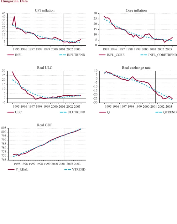
Figure 1 shows the historical path of the annualized rates of headline and core inflation, and of the logs of real unit labor cost, real exchange rate and real GDP. The dotted lines show Hodrick-Prescott filtered series, the vertical lines in the panels show the period of the switch in the monetary policy regime. Appendix A contains detailed description of these series and of additional series used in our estimations. The following remarks are worth noting.

Firstly, the time span considered is quite short: it represents a total of 37 data points. The choice of 1995Q1 as starting period was however constrained by the availability of necessary series. Note especially that core inflation and unit labor cost are both published since 1995 in Hungary. At the same time, the Hungarian economy has gone through a phase of deep insti-tutional changes during the first half of the ninties which have laid down the bases of a market economy. These changes were accompanied by increasing inflation and serious disequilibri-um problems in the economy. A Stabilization Program adapted in 1995Q1 restored internal and external equilibrium and introduced a crawling exchange rate peg monetary policy regime in the framework of which inflation could be fought. Market mechanisms have also been arguably stabilized by 1995. In spite of another switch in the monetary policy regime in 2001 Q2, the period since 1995 Q1 seems reasonably homogenous. These considerations support-ed our choice to model private agents’ price setting by rational profit maximizing behavior starting from that date.

Secondly, standard theoretical Phillips curves model business cycle frequency fluctuations of the inflation rate around some constant steady state. Hungarian aggregates seem however to evolve along a convergence path towards a new and unknown steady state. Moreover, this convergence process has been driven by structural changes of the transition process which are not captured by conventional price setting models.5

In addition, convergence to a lower long run inflation rate has arguably been a unique historic event which is not relevant for future short-run inflation dynamics. We have therefore chosen to abstract from convergence and to model the fluctuations of the inflation rate around its convergence path by standard models. A similar approach is adapted among others by COENEN ANDWIELAND(2005) for Spanish and Ita-lian data, by COENEN ANDLEVIN(2004) for German data, by RIBON(2004) for Israeli data and RUMLER(2005) to various euro-area countries.

We have chosen to use the Hodrick-Prescott filter with the standard smoothing parameter of λ=1600. The convergence path implied by this filter is very similar to the one implied by the alternative deterministic trend used by COENEN ANDWIELAND(2005) as shown in Figure 2. The

2. The data

4

Datasource: Magyar Nemzeti Bank (MNB) Quarterly Projection Model database, June 2004.

5

As noted e.g. in DARVAS ANDVADAS(2004), the economic downturn during the first half of the nineties has been matched by a massive rise in inflation, while the disinflation was accompanied by relatively high growth rates of real economic activity which is contrary to conventional wisdom.

impact of the use of a deterministic trend on our estimation results turned out to be of minor importance. We therefore only discuss results based on HP filtered series throughout the entire paper.6

We are aware that detrending is a shortcut, which may introduce various biases into our esti-mation results. First, as discussed in COENEN ANDWIELAND(2005), focusing on inflation devia-tions from trend would only be theoretically appropriate if the ‘source of the disinflation had been a credible, fully anticipated, gradually phased-in reduction in the policy makers’ inflation target.’ This has most likely not been the case in Hungary. However, COENEN AND WIELAND (2005) analyze the sensitivity of their estimation results to this implicit assumption and show that it does not imply significant distortions for the estimations.

Second, modeling the series’ deviations from their convergence path by standard models implicitly assumes that the convergence process has only influenced the long run dynamics of economic aggregates while leaving the business cycle frequency unaffected. This further sim-plification is another potential source of bias in our estimations. Modelling the effects of the convergence process on short-run inflation dynamics is however beyond the scope of the present paper. Instead, we check the sensitivity of our results to the filtering by reestimating all the considered specifications with unfiltered variables.

Throughout the entire paper, the core inflation rate will be used as the benchmark measure of the inflation rate.7

Hungarian core inflation rate is computed from the CPI by the exclusion of regulated prices, nonprocessed foods, market energy prices, privately owned housing servic-es.8

Regulated prices represented an important but decreasing part in the computation of the CPI over the sample period. By the exclusion of those prices, the core inflation rate seems a more accurate measure of Hungarian firms’ pricing behavior than the CPI. The robustness of our results to the choice of this indicator will be discussed by comparing them with results obtained using the CPI.

6

For a more detailed discussion of the implications of different detrending methods for New EU Member States business cycles see DARVAS ANDVADAS(2004).

7

Producer price index was not available in the MNB Quarterly Projection Model’s database.

8

In this section, we estimate traditional Phillips curves for Hungarian data and check the stabil-ity of our results.

The traditional Phillips curve is an aggregate relationship which describes short-run inflation dynamics by lagged values of inflation and some cyclical indicator. In addition, open econo-my extensions include some measure of external real shock. Denoting the inflation rate by π_t the cyclical indicator by x_tand the external variable by open_t, the Phillips curve is commonly specified as follows:

(1)

By using the inflation rate’s cyclical fluctuations around its long run convergence path instead of using the actual inflation rate series, we eliminate the long run from our estimations. The standard restriction for the Phillips curve’s long-run verticality, ∑h

i=1 βi=1 then becomes an inequality: ∑h

i=1 βi<1 This weaker restriction requires that inflation return to its long run path and thereby excludes explosive dynamics.

A real expansion (contraction) is expected to be positively (negatively) related to the inflation rate. The two alternative cyclical indicators we use are the output gap and the real unit labor cost.9

In this case, the coefficient λis expected to be positive.

Defining the external prices as the ratio of foreign prices over domestic prices, the sign of the open economy variable’s coefficient is expected to be positive.10

It might however be difficult to isolate the relationship between external variables and the inflation rate from the closed economy rela-tionship: real depreciation may increase domestic prices directly thereby decreasing aggregate demand; at the same time real depreciation can stimulate exports, hence increasing demand and thereby have an increasing effect on prices. Three alternative measures will be used in our esti-mations: the real effective exchange rate, real import prices and the terms of trade.11

The traditional Phillips curve is reported to describe post-war US and European inflation reason-ably well.12

The cyclical indicator seems to influence the inflation rate positively in the short run,

1 1 1 t i t i h i t i t i h i t

β

π

λ

x

γ

open

ε

π

=

+

+

+

∑

∑

3. Traditional Phillips curve

9

Alternatively, the unemployment rate and capacity utilization could also be used as cyclical indicators. We have run esti-mations using the unemployment rate – the results were very similar to those to be presented. Capacity utilization series were not available.

10

By definition, an increase in opentsignals a real depreciation.

11

For similar specifications see e.g. BALAKRISHNAN ANDLOPEZ-SALIDO(2002) and KARA ANDNELSON(2003).

12

See e.g. RUDEBUSCH ANDSVENSSON(1999), GALI, GERTLER ANDLOPEZ-SALIDO(2001), BALAKRISHNAN ANDLOPEZ-SALIDO(1999), KARA ANDNELSON(2003) for traditional Phillips curve estimations for US, euro area respectively UK inflation.

while long run verticality has also been confirmed by previous empirical studies. Evidence on the role of the external variable is however mixed: BALAKRISHNAN ANDLOPEZ-SALIDO(1999) find e.g. the external shocks to play a significant role in short-run UK inflation dynamics; in contrast, KARA AND NELSON(2003a) claim that the external variable has only played a minor role.13

Moreover, in spite of its apparent empirical success, the Lucas critique still remains an issue in traditional Phillips curve estimates: most empirical studies find the estimates to be structurally unstable.14

The results of traditional Phillips curve estimations for Hungary are summarized in Tables 1 and 2 for the closed resp. open economy specifications.15

The following results stand out.

First, the success of the closed economy specification depends on the cyclical indicator used. While the output gap does not appear to have sizeable effects on the inflation rate’s cyclical fluctuation, the real unit labor cost turns out to be significant. This is in contrast to estimations reported for US and euro-area data, where the output gap is significant in the estimated tradi-tional Phillips curve.16

Second, the exchange rate channel seems to be highly insignificant, independently of the choice of the external variables when one lag of the variables is included (see Table 2). The inclusion of further lags does not substantially change this conclusion: only the specification using three lags of the HP-filtered real import price shows evidence for a significant role of the external variable (see Table 2a).17

In addition, as already noted, due to the regime change in 2001Q2 , one needs to be particu-larly cautious about structural breaks in the estimations.

Formal Chow structural break tests performed for the closed economy specification indicate a significant structural break around the period of the regime change in the parameter estimates, independently of the cyclical indicator used.18

These results are confirmed by recursive and subsample estimations. The stability tests hence support the Lucas critique: the monetary pol-icy regime switch seems to have significantly influenced the parameters of the models. This fact should warn of using this specification for the evaluation of monetary policy. In what fol-lows, we therefore estimate New Phillips curves which are explicitly deduced from structural models and hence exempt from the Lucas critique.

13

Both papers study short-run UK inflation dynamics, the sample period and the external variable used are however dif-ferent. At the same time, KARA ANDNELSON(2003) report subsample estimations in support of the robustness of their claim over various periods.

14

See e.g. GGL (2001) and BALAKRISHNAN, LOPEZ-SALIDO(1999) for a more detailed discussion.

15

Trivially, in closed economy estimations γi=0. Estimation by OLS. Bresch-Pagan tests do not reject the homoscedastic-ity of the error term. Breusch-Godfrey serial correlation tests indicate residual auto-correlation at 10 % which is correct-ed for by the Newey-West error correction with 3 lags as implicorrect-ed by the standard formula.

16

See e.g. RUDEBUSCH ANDSVENSSON(1999), GG (1999) and GGL (2001).

17

Findings are somewhat different when non-detrended data are used. In this case, both the sum of coefficients of the change in real exchange rate and of the change in real import prices are significant when more than one lags are includ-ed. The effect remains however quantitatively small: the sum of these coefficients remains less than 0.2 in any case.

18

A number of recent studies have tried to solve instability problems arising in the traditional Phillips curve estimations for US and Euro-area data by elaborating structural models of short run inflation dynamics. This section outlines a closed economy New Hybrid Phillips curve, of two different open economy extensions of it and addresses empirical issues of New Phillips curve estimations. The next section presents estimation results.

4.1 CLOSED ECONOMY MODEL

The New Phillips curve is based on individual firms’ price setting behavior. The model that will be estimated is a version of the CALVO(1983) staggered price setting model extended to incor-porate backward looking price setting by a fraction of firms. This model has first been present-ed by GG (1999).19

There is a continuum of monopolistically competing firms in the economy, whose size is nor-malized to 1. As in the baseline Calvo model, each firm faces a probability ξof not being able to readjust its price in a given period. This probability is constant across firms and constant over time. In addition, GG (1999) assume two types of firms: a fraction 1–ωwho adjust their prices in a forward looking way, as in the baseline Calvo model, and a fraction ωwhich follow instead some backward looking rule-of-thumb in their price readjustment.

These assumptions imply that the average price level, p_tcan be expressed as:20

(2)

where p_tfix_{stands for the average of fixed prices, i.e. prices that have not been readjusted in} period t and p_t* denotes the average of newly set prices.

As in CALVO(1983), the average of fixed prices equals the average of the previous period gen-eral price level:

(3)

while the average of newly set prices is itself a weighted average of prices readjusted in a for-ward looking way, p_tf_{and of prices readjusted following the rule of thumb, p}

tb: (4)

)

1

(

p

p

p

=

−

ω

+

ω

=

p

p

−

+

=

p

p

p

ξ

(

1

ξ

)

4. New Phillips curve

19

For a comprehensive description see GG (1999).

20

Forward looking firms set their price to maximize their future flow of profits subject to the price setting rules. Denoting nominal marginal costs by mc_tn_{and the time discount factor by βthe} optimally readjusted price is:

(5)

Backward looking firms follow the a rule-of-thumb according to which they set their prices to the previous period average of newly set prices updated by the previous period inflation rate:

(6)

Although the assumption of backward looking price setting might be criticized, note that it can be motivated by some costs of information gathering which are exogenous to this model. Rule-of-thumb behavior can in this case be considered as a useful shortcut. In addition the rule-of-thumb as specified in equation (6) has several appealing features as pointed out in GG (1999). First, it implies no long-run deviation of backward looking prices from the reoptimized price if inflation is stationary. Second, the rule-of-thumb is not entirely backward looking in that, by the previous period newly set price index, it takes into account previous expectations about the future.

By combining equations (2) to (6), the New Hybrid Phillips curve can be expressed as:

(7)

The coefficients γ_b, γ_f, λare functions of deep parameters:

(8)

Note first, that the backward looking price leads to the inertia of the inflation rate. When there is a positive fraction of backward looking firms in the economy, the coefficient of lagged infla-tion rate is bigger than zero. At the extreme where all firms are forward looking, the Hybrid Phillips curve (7) reduces to the standard pure forward looking New Phillips curve.

)].

1(

1[

with

)

1

)(

1

)(

1

(

β

ξ

ω

ξ

φ

φ

φ

φ

βξ

ξ

ω

λ

βξ

γ

ω

γ

−

−

+

=

−

−

−

≡

≡

≡

γ

π

γ

E

π

λ

mc

π

=

+

+

+

=

p

p

π

)

(

)

(

)

1

(

E

mc

p

∑

−

=

βξ

βξ

Note further, that in this model, the sum of the coefficients of past and expected future infla-tion rates, γ_band γ_fis related to the time discount factor β: if β=1, then γ_b+γ_f=1. Since time units are measured in quarters, the discount factor is expected to be very close but not equal to 1. However, for plausible levels of ξand ω, the sum of γ_band γ_fremains reasonably close to 1.21

4.2 OPEN ECONOMY EXTENSIONS

Recent New-Keynesian literature has suggested various open economy models which differ in the way the relationship between the inflation rate and real exchange rate is captured: differ-ences concern assumptions made on the type of imported goods and on the resulting degree of exchange rate pass-through.22

Different specifications yield differences in the implied Phillips curves, too. Empirical Phillips curve estimations in general estimate one of the follow-ing models. One strand models imported goods as final consumption goods assumfollow-ing full pass-through of exchange rate variations on the general price level. The other strand models imported goods as intermediate consumption goods. In this setting, there is full pass-through of changes in the exchange rate on import prices, the pass-through on the general price level is however incomplete.23

In the case of Hungary, we have no reason to exclude a priori either of these specifications, therefore and for the sake of comparability, we chose to estimate both models as detailed below.

4.2.1 Imported final consumption goods

In this subsection, we extend the model presented in KARA ANDNELSON(2003) to the Hybrid Phillips curve setting.

Imported goods are specified as final consumption goods. The representative household’s consumption bundle is then a composite of domestically and externally produced goods. In addition, domestic price setters behavior is described by the GG price setting model. In this case, the evolution of the domestic inflation rate, π_td_{is described by the Hybrid Phillips curve:}

(9)

Following from households’ optimal choice between domestic and imported goods, the overall inflation rate, π_tcan be expressed as a weighted average of domestic and imported goods’ price inflation rate.24

Assuming full pass-through on the prices of imported consumption goods, the overall inflation rate can be written as:

1 1 t d t t f d t b d t

γ

π

γ

E

π

λ

mc

π

=

+

+

NEW PHILLIPS CURVE

21

If e.g. β=0.9, the value of γb+γf∈(0.95, 1) for ∀ξand ω.

22

For a comprehensive survey see LANE(2001).

23

For estimations of specifications with imported goods as intermediate goods see e.g. GALI ANDLOPEZ-SALIDO(2001), BALAKRISHNAN ANDLOPEZ-SALIDO(1999), KARA ANDNELSON(2003), RIBON(2004). Estimations of imported goods as final consumption goods are reported in KARA ANDNELSON(2003).

24

This expression can be deduced assuming monopolistic competition at home and abroad with an equal elasticity of substitution between differentiated goods within a region and a CES utility function over domestic and imported goods. See e.g. MONACELLI(2004).

where π_tm_{is the inflation rate of imported prices in foreign currency, Δe}

tis the depreciation rate of the domestic currency and s stands for the share of imported prices in the inflation rate of the general price level. Defining the real exchange rate as q_t=p_tm_+e

t–ptdand rearranging we get:

(10)

where Δq_tis the rate of change of the real exchange rate. Defined in this way a rise (decrease) in q_tshows the real depreciation (appreciation) of the domestic currency. Restricting γ_b+γ_f=1 and substituting expression (10) into the Phillips curve (9) yields the cumbersome expression:

(11)

The inflation rate hence depends on the current and the future expected change of the real depreciation rate. The sign of the current change of real depreciation rate is expected to be positive, while that of the future expected change in the real depreciation rate is expected to be negative.

4.2.2 Imported intermediate production goods

As an alternative, we follow MCCALLUM ANDNELSON(1999) to model imported goods as inter-mediate production goods while all final goods are produced domestically. This specification modifies the definition of real marginal cost in the Phillips curve. The real exchange rate there-by enters the Phillips curve in levels and not in differences.25

Formally the model can be deduced as follows.

To keep things simple, we assume a Cobb-Douglas production technology:26

where z_tis a labor-augmenting technology shock and y_tm_{is an index of imported} differentiat-ed intermdifferentiat-ediate production goods. Note that y_tstands here for gross output and the parame-ter αis therefore the labor’s share in gross output as opposed to the usual labor’s share in GDP.27 m t t t t

z

l

y

y

=

α

(

+

)

+

(

1

−

α

)

,

.

)

(

)

(

γ

E

π

γ

π

s

γ

E

q

q

s

γ

q

q

λ

mc

π

=

+

−

Δ

−

Δ

+

Δ

−

Δ

+

,

= π

−

s

Δ

q

π

),

(

)

1(

=

−

s

π

+

s

π

+

Δ

e

π

For a slightly different specification see e.g. BALAKRISHNAN ANDLOPEZ-SALIDO(1999) or GALI ANDLOPEZ-SALIDO(2001).

26

Variables expressed in deviation from steady state.

27

Assuming the price of one unit of the imported composite good is p_tm_+e

t, the real marginal cost can be expressed as:

(12)

where w_tstands for real wage and q_tis the real cost of a unit of the imported good. Substituting this expression into the closed economy Hybrid Phillips curve (7) gives:

(13)

The expressions linking γ_b and γ_f to the structural parameters are as in expression (8), φ remains unchanged as well. The coefficient of real unit labor cost, and real exchange rate are:

(14)

4.3 EMPIRICAL ISSUES

This subsection discusses some empirical issues concerning the estimation of New Phillips curves in general and their estimations for Hungarian data in particular. We first discuss the choice of the estimator, then the choice of the cyclical indicator and last the choice of the instrument set used in our estimations.

4.3.1 Estimator

We will use a single equation instrumental variable estimator in our New Phillips curve estimations.

The use of this method has been criticized by RUDD AND WHELAN (RW, 2001) and by LINDE (2002). Both claim that the GMM estimation introduces a bias on the weight of the past infla-tion rate in the Phillips curve.28

In addition, as shown by LINDE(2002) the GMM method implies changes in structural parameters when monetary policy changes. Linde suggests the use of full information estimation techniques to avoid these problems.

Our choice of estimator can be sustained by the following arguments.

.

)

1

)(

1

)(

1

)(

1

(

;

)

1

)(

1

)(

1

(

φ

βξ

ξ

ω

α

λ

φ

βξ

ξ

ω

α

λ

−

−

−

−

≡

−

−

−

≡

.

)

(

γ

E

π

γ

π

λ

w

z

λ

q

π

=

+

+

−

+

,

)

1

(

)

(

w

z

q

mc

=

α

−

+

−

α

NEW PHILLIPS CURVE

28

While both studies agree on the fact that the GMM introduces a bias, they contradict each other on the predicted sign of the bias. RW (2001) argue that GG underestimate the weight of backward looking behavior, in contrast, LINDE(2002) claims that single-equation GMM tends to overestimate inflation inertia. See RW ANDLINDE(2002) for a comprehensive discussion.

First, the use of the instrumental variable estimator makes our results directly comparable to a large number of previous studies which have used single-equation Generalized Method of Moments (GMM).29

Second, the criticisms concerning the bias introduced by the GMM estimator have been refused by GGL (2003) as being ‘plainly incorrect’. They further argue that full information methods have their own drawbacks when some of the equations are not correctly specified. Note that, in the case of Hungary, the use of full information methods seems to be particularly problematic. Especially, the specification of a monetary policy equation appears to be difficult first, because, as already noted, there has been a shift in the monetary policy regime in 2001; and also because monetary policy does not seem to have followed any stable underlying reac-tion funcreac-tion over the sample period.

While we thus stick to the instrumental variables technique, the Two Stage Least Squares (2SLS) estimator has been preferred to the more widely used efficient GMM estimator because of the shortness of available series. The efficient GMM estimator can be shown to be consis-tent and to achieve the lower bound of estimates’ asymptotic variance. However, the small sample properties of this estimator are likely to be poorer than those of methods not using fourth moment estimates, like the 2SLS. In addition, in the case of homoskedasticity, the 2SLS estimator corresponds to the efficient GMM.30

To check for the Linde’s critique about the estimation’s structural stability, we will perform recursive regressions.

4.3.2 Cyclical indicator

The structural Phillips curve links inflation dynamics to the real marginal cost directly. The expression of real marginal costs depends on the specification considered and on the produc-tion funcproduc-tion assumed.

In the closed economy model, the assumption of Cobb-Douglas technology implies where is the real unit labor cost, and α_nis the labor’s share parameter in the produc-tion funcproduc-tion. In percentage deviaproduc-tion from steady state, this can be expressed as mc_t=s_t which suggests the use of real unit labor cost’s deviation from its steady state in the estima-tion of the New Phillips curve.31

In the open economy model with imported goods specified as intermediate production goods, the real marginal cost takes is given by (12). KARA ANDNELSON(2003) suggest the use of real

t t t t Y P N W t S≡ n t S t MC= α 29

Notably, GG (1999) and GGL (2001) have used GMM.

30

See e.g. HAYASHI(2000) Chapter 3.

31

unit labor cost as a proxy for productivity-shock-deflated real wages (ω_t–z_t). For the real price of the imported goods we use real effective exchange rate.32

As an alternative to real unit labor cost, the Phillips curves will also be estimated using the out-put gap as cyclical indicator. Theoretically, the outout-put gap can be used to this end if it is pro-portional to the real marginal cost, i.e. mc_t=κy_t, with κ>0 being the constant output elasticity of real marginal cost. Empirical studies show however the output gap to perform much more poorly than real marginal cost in US and Euro-area Phillips curve estimations.33

One of the rea-sons pointed out for the failure of New Phillips curve estimations based on the output gap is that the proportionality between the output gap and the real marginal cost does not seem to be confirmed by the data. Instead of moving contemporaneously with the output gap, the real marginal cost is reported to lag the output gap over the cycle.34

A comprehensive discussion of this issue is beyond the scope of the present paper. It should sim-ply be noted that in Hungarian data, the real unit labor cost seems to be relatively synchronized with the output gap compared with US data.35

The dynamic relationship between these variables does hence not give clear indications for whether the unit labor cost might perform better in esti-mations compared to the output gap. We will present the results of estiesti-mations using real margin-al cost and discuss the robustness of these results to replacing marginmargin-al cost by the output gap.

4.3.3 Instrument set

The performance of the 2SLS estimator, as that of any other instrumental variable estimator, crucially depends on the relevance of instruments.36

As discussed in SHEA(1996), ‘relevance in a multivariate context requires that the instrument set have components important to the endogenous explanatory variable that are linearly independent of those important to exoge-nous variables included into the regression’. This means that the instrument set is relevant if it can explain a large enough fraction of the endogenous explanatory variables’ variance while being uncorrelated with the exogenous explanatory variables included in the regression. Thereby, the instruments explain the dependent variable’s variance directly and not only indi-rectly via the exogenous explanatory variables’ variation. Shea suggests to use the partial R2 and the adjusted partial R2_{statistics to check for the relevance of instruments.}37

Appendix B contains a desciption of the computation of these indicators.

NEW PHILLIPS CURVE

32

We checked the robustness of our estimations by reestimating the open economy specifications using real import prices. Our results turned out to be very robust. Results not displayed are available on request from the author.

33

The choice of output gap vs. real unit labor cost and different specifications of the supply side have been extensively debated in recent literature. See e.g. SBORDONE(2002), GG (1999), NEISS, NELSON(2002), GALI(2005) for some examples.

34

See e.g. GALI ANDGERTLER(1999). Another plausible reason for the insignificance of the output gap might be the inappro-priate measure of the output gap in empirical studies. For a more detailed discussion see also NEISS ANDNELSON(2002).

35

GALI, GERTLER(1999) report negative correlations of the current output gap with current and lagged real unit labor cost. In contrast, in Hungarian data, current output gap is correlated positively not only to leads of the real unit labor cost but also to contemporaneous ulc and to its lags up to lag 3 (quarterly data). Results based on HP filtered ulc.

36

See e.g. NELSON, STARTZ(1990).

37

In most Phillips curve estimations, the instrument set contains lags of explanatory variables. Such an instrument set turns out, however, to perform poorly on Hungarian data. We therefore used a broader set of instruments. The benchmark instrument set used in our estimations con-tains, in addition to a constant term, two lags of the inflation rate, real unit labor cost, wage inflation, budget deficit to GDP ratio, non processed food price inflation rate and of real depre-ciation rate.38

In the closed (open) economy model, this instrument set has a partial R2_{of 0.63} (0.50) and an adjusted partial R2_{of 0.37 (0.16).}39

The robustness of our results to the choice of the instrument set will be discussed in Section 6.

38

All variables in deviations from HP trend except the real GDP growth rate.

39

Instrument sets include all included exogenous variables. The partial R2_{for the expected future real depreciation in the} imported final consumption goods specification is 0.25. Estimations using HP filtered CPI include the same variables: Partial R2_{=0.25. For estimations using non detrended core inflation rate, we used the same variables without} detrend-ing them. Partial R2_=0.57.

This subsection reports estimates of the closed economy model and of its two open economy extensions. We first discuss the linear estimations of the Phillips curves and then present results for the models’ structural parameters. To our knowledge, these are the first structural Phillips curves estimated for a new EU member state.40

5.1 REDUCED FORM

This subsection reports estimates of equations (7), (11) and (13). Following GALI ANDGERTLER (1999), these estimates will be referred to as ‘reduced form’ since the coefficients of the vari-ables entering these Phillips curves are estimated directly without the identification of the underlying behavioral parameters β, ξ, ω.41

Assuming expectations of forward looking producers are rational, the error term is uncorrelated with information dated t or earlier. The following orthogonal-ity conditions can then be estimated by instrumental variables for the above described models:

Closed economy:

(15)

Open economy imported final consumption goods:

(16)

Open economy imported intermediate goods:

(17)

where z_tdenotes the vector of instruments containing only contemporaneous or past values of variables.

The first lines of Tables 3a, 3b and 3c show the results of our estimations of equation (15) using HP filtered core inflation and HP filtered real unit labor cost as a proxy for real marginal cost’s deviation from the steady state resp. for technology shock deflated real wages. In addition, tables 3a and 3c display results of estimations with the restriction γ_f+γ_b=1.

.

0

}

)

)

(

{(

−

−

−

−

−

=

w

z

q

E

π

γ

π

γ

π

λ

λ

z

.

0

}

)

)

(

)

(

{(

−

−

+

−

−

−

−

=

s

q

q

s

q

q

mc

E

π

γ

π

γ

π

γ

Δ

Δ

γ

Δ

Δ

λ

z

,

0

}

)

{(

−

−

−

=

mc

E

π

γ

π

γ

π

λ

z

5. Estimation

For earlier New Phillips curve estimates for EU accession countries see ARRATIBEL ET AL. (2002). For Hungarian estima-tions see HORNOK, JAKAB(2003). These authors only estimate reduced form coefficients.

41

We do not show separately the results of the estimations assuming purely forward looking inflation dynamics. As already noted however, the hybrid Phillips curve nests the purely forward looking Phillips curve for ω=0⇔γ_b=0.

The following diagnostic tests have been performed.

First, the model’s overidentifying restrictions were tested. Hansen’s J test does not reject the overidentifying restrictions and hence the specification of the model in any of the estimations. Note, that while the reported results were estimated by the weighting matrix (ZZ’)–1_{, this test is} performed using the efficient weighting matrix. As noted above, the two estimators correspond in case of homoskedasticity. Testing for homoskedasticity in the case of 2SLS estimator is not straightforward.42

We have therefore reestimated the equation with the optimal weighting matrix and checked for the differences in point estimates. The differences turned out to be of minor importance.43

This seems to support conditional homoskedasticity. In addition to this informal comparison, a more formal modified Breusch-Pagan test was conducted. The Breusch-Pagan test requires the auxiliary regression of the squared residuals on the regression’s exogenous variables to be insignificant. The above regression includes however an endogenous variable. The squared residuals have therefore been regressed on all included and excluded exoge-nous variables. This test confirmed our intuition: conditional homoskedasticity of residuals can-not be rejected (closed economy: p=0.626, open economy imported intermediate goods: p=0.24).

Tests of residuals’ serial correlation find significant autocorrelation. The Ljung-Box test as well as a Breusch-Godfrey test modified in the same way as the Breusch-Pagan test previously, reject the null hypothesis of no serial correlation at any usual significance level. GALI, GERTLER, LOPEZ-SALIDO (2001) encounter the same problem. They argue, that the serial correlation of residuals might be due to the fact that the hybrid Phillips curve model does not fully capture all the dynamics in the present data. One reason for this might be that the backward looking price adjustment takes into account more than one lagged value of inflation. We therefore tried to include up to eight lags of inflation into the Phillips curve equation. As it turned out, the addi-tional lags were often not significantly different from zero, while both the Ljung Box and the modified Breusch-Godfrey test continued to reject the null hypothesis of no serial correlation at least five percent.44

Instead of modifying the specification, we corrected for serial correla-tion in the original specificacorrela-tion by the use of a 3 lag Newey-West estimate of the covariance matrix.

Finally, we have tested for the exogeneity of unit labor cost and of lagged inflation in both the closed and open economy models and for the exogeneity of the real exchange rate in the open economy model with imported intermediate goods. The test of a subset of orthogonality con-ditions does not reject the exogeneity of these variables at any usual significance level.

Overall, the reduced form estimations are quite encouraging. The following results are worth to be noted.

42

See e.g. HAYASHI(2000) Ch.3. p. 234.

43

The estimates of gb and gf were changing less than 0.01 in all specifications. Changes in the estimate of the slope coef-ficients λand of λl_{and λ}m_{are smaller than 0.03.}

44

First, the coefficients of future expected inflation rate, of lagged inflation rate and of real unit labor cost enter the equations with the expected sign in all specifications although the unit la-bor cost coefficient is not significant. In addition, as shown in the last columns of table 3a and 3c, the hypothesis that the inflation coefficients sum to 1 cannot be rejected.45

This suggests, that the discount factor is reasonably close to 1, as can be expected in a quarterly model. In addition, as displayed in Figures 3a and 3b, fitted values of the core inflation based on the closed economy and the intermediate goods open economy model show that the Hybrid Phillips curve explains Hungarian inflation dynamics reasonably well. Although the timing of predicted smaller amplitude oscillations sometimes misses the actual dynamics, larger ampli-tude oscillations are tracked quite well by both models.

Second, estimates indicate a roughly equal weight of expected future inflation and of lagged inflation in the determination of current inflation, with a small edge for future expected inflation. This finding is opposed to results reported for US and Euro-area data by GG (1999) and GGL (2001) according to which, the forward looking term dominates short-run inflation dynamics in both of these regions; at the same time, our results are similar to results found for pooled New EU member states data by ARRATIBEL ET AL. (2002) as well as to e.g. Spanish inflation dynam-ics estimations by GALI ANDLOPEZ-SALIDO(2001) and also to Israeli inflation dynamics present-ed in RIBON(2004).46

Third, the imported intermediate goods specification seems to be a better description of Hungarian inflation dynamics than the imported final consumption goods specification. While the real exchange rate coefficient takes the expected sign in the estimation of equation (17), the change of real depreciation in equation (16) is not only highly insignificant, but its sign restrictions cannot be confirmed either. These findings are in line with those reported in KARA ANDNELSON(2003 and 2003a) for UK data. The authors explain the better performance of the imported intermediate goods open economy model by the fact that import prices are more closely related to exchange rate changes than final consumption prices. A similar pattern can also be found in Hungarian data.47

Fourth, as can be seen in the tables, the filtering has very little influence on our results. The point estimates of all the coefficients in all specifications are almost not modified when unfil-tered data are used for the estimations.

ESTIMATION

45

This result also holds for the imported final consumption goods specification. There, the restriction implied so little changes that we decided not to show the results.

46

SMETS ANDWOUTERS(2003) and (2004) confirm GGL (2001) results for the euro area using a FIML estimation technique. COENEN ANDWIELAND(2005) also find a relatively high lagged inflation coefficient for Spanish inflation dynamics. BENIGNO ANDLOPEZ-SALIDO(2002) report relatively high inflation inertia for Spain and Italy and predominantly forward looking dynamics for Germany. For various euro-area member state estimates see also RUMLER(2005). Rumler’s findins are somewhat different.

47

The contemporaneous correlation of the change in nominal effective exchange rate with the core inflation rate is -0.02, while its correlation with the change in the import price is 0.54. Both computed for filtered data. For a more detailed dis-cussion of exchange rate pass-through in Hungary see DARVAS(2001).

Finally, as displayed in table 3a lines 5 to 8, our main conclusions remain unaffected when the CPI inflation is used instead of the core inflation and also when the output gap is used instead of real unit labor cost.48

5.2 STRUCTURAL FORM

This section tries to recover the New Hybrid Phillips curve’s deep parameters, β, ξand ω. These parameters mainly concern the price setting behavior of agents and thereby allow to draw conclusions with regard to mechanisms leading to inflation inertia. As shown by the high weight of lagged inflation in the reduced form estimations of the Hybrid Phillips curve, this issue is particularly relevant to Hungarian inflation dynamics.

Results are presented for the closed economy model and for the open economy extension specifying imported goods as intermediate production goods. The discussion is based on esti-mations using HP filtered data.49

Formally, we substitute the structural parameters for the reduced form parameters in the New Hybrid Phillips curve described by relation (7) and (13) according to the functions (8) resp. (14). It is known that small-sample nonlinear instrumental variable estimations are sensitive to the precise specification of orthogonality conditions.50

We therefore follow GG (1999) and GGL (2001) to estimate two alternative variants of the orthogonality condition: in the first specifica-tion, the coefficient of current inflation is not normalized, while in the second specification it is normalized. For the closed economy model we hence estimated the following two equations.

The specification in which the inflation rate coefficient is not normalized:

(18)

The normalized specification:

(19)

The equations estimated for the open economy are as follows.

The specification in which the inflation rate coefficient is not normalized:

(20)

−

−

−

−

−

−

−

ulc

E

{(

φπ

βξπ

ωπ

α

(

1

ω

)(

1

ξ

)(

1

βξ

)

−

(

1

−

α

)(

1

−

ω

)(

1

−

ξ

)(

1

−

βξ

)

q

)

z

}

=

0

.

.

0

}

)

)

1

)(

1

)(

1

(

{(

−

−

−

−

−

=

−

mc

E

π

φ

βξπ

φ

ωπ

φ

ω

ξ

βξ

z

.

0

}

)

)

1

)(

1

)(

1

(

{(

−

−

−

−

−

−

=

mc

E

φπ

βξπ

ωπ

ω

ξ

βξ

z

These results equally hold for the open economy specifications which we did not display separately.

49

In general, the results were very little affected by the filtering. Noteworthy differences will be discussed in footnotes.

50

The normalized specification:

(21)

Our estimation results are summarized in Tables 4a and 4b. The first four lines in each table show results based on HP filtered data. Lines 5 to 8 show results obtained using unfiltered data. The first three columns in the table show the estimates of the structural parameters. Columns 4 to 6 (7 for the open economy model) give the estimates of the resulting reduced form parameters. We also show Hansens’s J test resp. its significance level in both tables.

Overall, the estimation results seem reasonable.

The estimate of the discount factor β is rather low in the not normalized specifications and rather high in the normalized specifications. Note however that these estimates are very impre-cise. We therefore reestimated the Phillips curves restricting the discount factor to a theoreti-cally plausible level of β=0.99. This cannot be rejected at five percent or less in any of our esti-mations while the restriction improves the estimation of other parameters. Wald restriction tests with the null hypothesis β=0.99 are displayed in the last two columns of table 4a for the closed economy and in table 4c for the open economy.

In addition to the closed economy structural parameters, the open economy model includes the additional parameter α, which stands for labor’s share in gross output. We have first esti-mated the above specifications without restricting αto a particular value. The estimate of α was in the interval of 0.63–0.82, the standard errors of the estimates were however very big. Since we are more interested in recovering the parameters of the price setting itself, we chose to calibrate this parameter to α=0.7.51

This restriction significantly reduced the standard error of our estimates. The robustness of our results to this calibration will be discussed in the next section.

The price setting parameters ωand ξare estimated at a significance level of less than 1 per-cent in all specifications. Nevertheless, standard errors are relatively large. Two features seem interesting to note.

First, the estimates support the importance of backward looking price setting behavior in Hun-gary as measured by the fraction of backward looking firms, ω. This parameter is found to be in the interval of 0.3–0.55. Estimates of this parameter seem to change very little between closed and open economy specifications. Despite the large error bands, all specifications

−

−

−

−

−

−

−

ulc

E

{(

(

1

)(

1

)(

1

)

βξπ

φ

ωπ

φ

α

ω

ξ

βξ

φ

π

−

φ

(

1

−

α

)(

1

−

ω

)(

1

−

ξ

)(

1

−

βξ

)

q

)

z

}

=

0

.

ESTIMATION

This value cannot be rejected at any usual significance level in any of our estimations. The interval based on filtered data is smaller and also contains 0.7. RIBON(2004) sets α=0.5 for Israeli data, while GALI ANDLOPEZ-SALIDO(2001) set

imply significantly greater fractions of backward looking price setters than those reported for the Euro-area by GGL (2001).52

Note that, according to the estimation of the normalized spec-ifications (19) and (21), more than half of the firms follow a rule-of thumb behavior.

Second, the probability of fixed prices ξis relatively low: the probability in any period that a firm cannot reset its price is indicated to be between 45 to 60 percent in the open economy model, and between 0.5 to 0.65 in the closed economy model. This is significantly lower than in comparable euro-area estimates.

Resulting implied estimates of reduced form coefficients support the relatively high degree of inflation inertia in Hungary. The real marginal cost coefficients are of the expected sign in all specifications. In addition, estimates of the normalized specifications show the slope coeffi-cients λl_{and λ}m_{to be at more than one standard error distance from zero. The coefficient of} the real exchange rate lies between 0.02 and 0.1, which is rather low; at the same time, simi-lar findings were reported in comparable previous studies.53

It should be noted, that the degree of inflation inertia might be overestimated. To see why, note that the coefficients of real marginal cost are not significant in our estimations. This might be due to a downward bias introduced by the poor quality of our proxy for real marginal costs. Since the coefficient of real marginal cost is inversely related to the parameters of price and inflation rigidity ωand ξ, if the real marginal cost is not significant, the nominal rigidity param-eters will automatically be biased upward in our estimations.54

Comparing our estimation results to microeconomic evidence yields some further support in favor of the overestimation problem. RATFAI(2000) studies the price setting behavior of various Hungarian stores over the period of 1993 to 1996 and finds that stores keep their prices fixed on an average for 3.42 months, i.e. a little longer than one quarter. The average price duration can be computed in the New Phillips curve model as . The resulting average duration lies between 1.77 and 2.71 quarters according to our estimates which represents a longer than that indicated by microeconomic evidence.

The overestimation problem does however not seem to be too important.

First, the bias is arguably not very large. As shown e.g. in DOTSEY, KING ANDWOLMAN(DKW, 1999), the higher the average inflation rate in a country, the lower the duration of prices tends to be. Since the findings of Ratfai are reported for a period when the average inflation rate has been higher than over the sample period of the current estimation, we have reason to assume that the average duration of prices may have somewhat increased since Ratfai has established his results.

1−1ξ

=

D

52

Estimates reported by GGL (2001) for the same specification on euro area data are: Not normalized specification: ω=0.024 (0.122), ξ=0.907 (0.015). Normalized: ω=0.335 (0.129), ξ=0.922 (0.031). (Standard errors are shown in brackets.)

53

See e.g. BALAKRISHNAN ANDLOPEZ-SALIDO(2001), KARA ANDNELSON(2003), RIBON(2004).

54

Moreover, the overestimation problem concerns most of the other structural Phillips curve esti-mations to which we compare our results. Note especially, that the slope coefficient of the Euro-area hybrid Phillips curve, as reported by GGL (2001) for the same specification, is not significantly different from zero55

either and that the average price duration implied by these specifications is also relatively high (10 to 12 quarters).56

GGL (2001) introduced a decreasing returns to scale production technology to improve estimation performance. The same modifi-cation did not improve results in Hungarian estimations. Moreover, our ξand D estimates are found to be relatively low, and the ωrelatively high, even compared with GGL’s presumably less biased results. Our estimations therefore seem to support that Hungarian inflation is sig-nificantly more sluggish than Euro-area inflation. The major reason leading to Hungarian infla-tion inertia, seems to be pervasive backward looking behavior, while prices are more often reset than in the Euro-area.

The difference between closed and open economy estimation results is rather small. The open economy estimation appears to slightly decrease the overestimation bias in the average price duration. This might be due to the an improvement of the real marginal cost measure when the real exchange rate is included. Other coefficient estimates are not much affected.57

Note finally, that our findings are similar to structural Phillips curve estimates for other coun-tries with a relatively high average inflation rate over the sample period. RIBON(2004) similarly finds that Israeli firms reset their prices relatively often with a relatively high weight of backward looking behavior, compared with US and euro-area data. GALI ANDLOPEZ-SALIDO(2001) report even higher estimates for Spanish firms’ backward looking fraction. These findings suggest that the behavior of firms depends on the state of the economy as argued e.g. in DKW (1999). Since the state of the economy has undergone important changes between 1995 and 2004 in Hungary, it is useful to examine the stability of our estimations. This will be discussed in the next section.

ESTIMATION

55

GGL (2001) report the following estimates. Specification 1: λ=0.018 (0.012). Specification 2: λ=0.006 (0.007). (See Table 2, lines 3 and 4 in their paper).

56

It should be noted, that this is not the preferred specification of GGL (2001).

57

Note, that for results based on unfiltered series, the open economy model implies a bigger improvement: estimations of specification (1) of the closed economy model are not converging while for the open economy model all estimation are converging.

We check the robustness of our estimates in three ways. First, we test the stability of our param-eter estimates with regard to structural breaks. Second, we show how the choice of different instrument sets influences our results. Last, we briefly discuss the effect of our calibration.

6.1 STRUCTURAL STABILITY

This subsection shows recursive estimations to check for the stability of our coefficient esti-mates over time. Since our conclusions are not affected by the particular specifications, we restrict our discussion to the outcome of the stability check for our preferred specification, i.e. the open economy model with imported goods specified as intermediate production goods. The terminal date goes from T=2000Q1 to 2004Q1. Figure 4a shows coefficient estimates of the structural parameters ωand ξfor specification (20), figure 4b displays those for specifica-tion (21). The upper line in each figure displays results of unrestricted estimaspecifica-tions, the bottom line those of estimations restricting β=0.99.

The estimates seem to be quite stable over the sample period.

The coefficient estimates of ξlie well within the error bands in all displayed specifications over the entire sample period. Estimates of the fraction of backward looking firms appear to be slightly decreasing over the period. The point estimate of ωis 0.38 in specification (1) and 0.7 in specifi-cation (2) over the period of 1995Q1 to 2000Q1 while it is 0.32 resp. 0.52 over the full sample. Note however, that the highest estimates are obtained for estimations based on a very short sample, these results are hence to be treated with caution. Moreover, the error bands are quite large, and these changes are not significant. We hence conclude that our estimates are reasonably stable.

6.2 INSTRUMENT SETS

As already discussed, the appropriate choice of the instrument set is essential in instrumental variable estimations. So far, we have described our results for estimations using always the same set of instruments. At this place, we discuss the way in which the use of different instru-ment sets influences our estimation results.

New instrument sets either include additional variables or additional lags of already used vari-ables. Appendix C describes the variables contained in each instrument set along with the sets’ partial R2_{indicators for the closed and the open economy models.}58

The benchmark

58

Formally, the the instrument set has to contain variables dated t or earlier to ensure Cov(εt+1; zt) = 0. As discussed in GGL (2001), when the marginal cost is measured with noise, it may be more appropriate to include only lagged values of the instrumental variables. We have followed this for our benchmark instrument set. Some of the alternative instru-ment sets contain however contemporaneous variables. Since we test the validity of our instruinstru-ments, this should not be too big a problem.

instrument set is Set 1 with a partial R2_{of 0.63 for the closed economy and 0.5 for the open} economy model. The partial R2_{s of alternative instrument sets lie in the range of 0.28–0.57 for} the closed economy model and in the range of 0.12 to 0.44 for the open economy setting.

The conclusions of our test turned out to be independent of the particular specification esti-mated. Figure 5 shows estimation results of specification (20) of the open economy model with imported intermediate production goods with the time discount factor restricted to 0.99. In each panel, we shaded the area between the minimum and the maximum value of the point estimates.

As can be seen in the figure, neither estimates of the deep structural parameters, nor the implied reduced form parameters are much influenced by the choice of the instrument set. In particular, all estimates of each coefficient lie within one standard error distance from other estimates of the same coefficient. Note that the point estimates of ωand γf_{implied by the} benchmark instrument set, lie within the range of estimates with different instrument sets. At the same time, the estimates of ξseem to be at the lower edge of estimates using different instrument sets, while those of the slope coefficients λl_{and λ}m_{lie at the upper edge.}

Overall, the differences are rather small. Especially, all the main conclusions remain unchanged by the use of any alternative instrument set.

6.3 CALIBRATION

This subsection discusses the robustness of our estimates to different values of the labor’s share coefficient.

First, we tested the benchmark calibration of α=0.7 in our estimations with each instrument set. The significance level of formal Wald restriction tests lies between 0.88 and 0.98 for all estima-tions.

Second, we reestimated the model using the benchmark instrument set, alternatively setting α=0.6 and α=0.8 The effect of these calibrations on our point estimates turned out to be neg-ligible. The changes in the estimates of deep parameters were less than 0.05. Changes in the deduced reduced form parameters were even smaller. Note especially that the coefficients of both real unit labor cost and of the real exchange rate remaine positive, independently of the value of the labors’ share parameter.59

ROBUSTNESS

59

In this paper, we estimated different Phillips curve models to describe Hungarian inflation dynamics over the period 1995Q1 to 2004Q1. Our results suggest that, while estimates of the traditional Phillips curve are subject to the Lucas critique, the standard New Hybrid Phillips curve and an open economy extension of it specifying importe