Facultad de Ciencias Econ ´omicas y Empresariales Universidad de Navarra
Working Paper n
◦
07/03
Welfare and Output in Third-Degree
Price Discrimination: a Note
Francisco Galera
Facultad de Ciencias Econ ´omicas y Empresariales
Universidad de Navarra
Welfare and Output in Third-Degree Price Discrimination: a Note Francisco Galera
Working Paper No.07/03 May 2003
JEL Codes: D43, D60, L13
ABSTRACT
In this note I provide examples to show that, contrary to what is widely believed, when changing from an uniform price to a third-degree price discrimination situation, an improvement in welfare is possible with output reduction, if there is more than one firm.
Keywords: price discrimination, imperfect competition, welfare
Francisco Galera Universidad de Navarra Departamento de Econom´ıa Campus Universitario 31080 Pamplona fgalera@unav.es
I
Introduction
One of the well-known conclusions about the welfare effects of third-degree price discrimination by a mo-nopolist is that “an increase in total output is a necessary condition for welfare improvement.” To avoid rep-etitions, this affirmation is called “proposition WO,” or simply, “WO.” Schmalensee (1981), Varian (1985), and Schwartz (1990) proved WO with different levels of generality. The purpose of this note is to show that, although WO is valid for a monopolist, it is not extendable to every situation with more than one firm.
To my knowledge, although the welfare effects of third degree price discrimination when competition is present have been studied, WO has never been seriously challenged (see Appendix 2). And there is a widely held view that WO is true more generally. See, for example, Stole (2001, p.9), Armstrong and Vickers (2001, pp.582-3) and Layson (1994, p. 323).
The logic of WO is clear. There is a consumer inefficiency associated with third-degree price discrim-ination: output is not optimally distributed to consumers because their marginal utilities will be unequal. Proposition WO asserts that the only way to overcome this consumer inefficiency is a sufficient increase in total output. This is true when there is only one firm or when all the firms share the same costs. But, with heterogeneous firms, costs saving by a better redistribution of output among firms can also overcome the consumer surplus inefficiency. When this is the case, it is no longer true that if output falls when price discrimination is introduced, then welfare must also fall.
I believe that the examples that follow are pertinent because the message of proposition WO, even if very probable, is based on one of two unlikely facts in real world: there exists pure monopolies, or all firms in an industry share the same costs. More research is needed to get conditions for proposition WO to be valid when there are heterogeneus firms.
II
The examples
A dominant firm with zero cost produces a single final product and sells it directly to consumers. Consumers are partitioned into two markets and the dominant firm faces Cournot competition only in one of its two markets from other firm with constant marginal costs, c. The inverse demand functions are Qb=a−paand
Qb=b−pb. We get the following proposition:
Proposition 1: Neither an increase in the dominant firm’s output, nor an increase in total output is a
necessary condition for welfare to improve.
Proof. See the following two examples and Appendix 1.
Example 1. This example shows that a change from uniform pricing to price discrimination causes a
welfare improvement with a reduction of the dominant firm’s output, although total output increases. The dominant firm, Firm 1, sells to two separate markets, A and B. Let us denote its output by qaand qb. Demand
in market A is Qa=18−pa, and in market B is Qb=10−pb. In market A there is another firm, Firm 2,
that competes with Firm 1 in quantities. Let us denote by xa its output. Costs are zero for both firms. In
Appendix one it is shown that, if Firm 1 is restricted to a uniform price, the equilibrium values, where the superscript U means uniform pricing, will be qUa =6.8, xUa =5.6, qUb =4.4; price and welfare (profits plus consumer surplus) will be: pU=5.6 and WU=180.64. Firm 1’s total output is QU1 =11.2. If Firm 1 can price discriminate, then the equilibrium values are (where the superscript D means price discrimination): pa=6, pb=5, qDa =6, xDa =6, qDb =5 and WD=181.5. Output of Firm 1 is QD1 =11. Welfare is increased
under price discrimination with lower output by Firm 1.
Example 2. This example shows that, with total output reduced, there is an increase in welfare. In this
example, I change demands, and cost of Firm 2. Everything else, notation included, is the same. Demand in market A is Qa=15−pa, and in market B is Qb=18−pb. Firm 2 has marginal cost 6. Again, it is easy
to see that, under uniform pricing, the equilibrium values will be pU=7.8, qUa =5.4, xUa =1.8, qUb =10.2, WU=202.86. Total output is QU =17.4. If Firm 1 can price discriminate, then the equilibrium values are: pa=7, pb=9, qDa =7, xDa =1, qDb =9 and WD=203.5. Total output is QD=17. Welfare is increased
under price discrimination with lower total output.
Now I provide an example with price competition instead of Cournot competition. A dominant firm with zero cost produces a single final product and sells it directly to consumers. Consumers are partitioned into two markets and the dominant firm faces price competition only in one of its two markets from other firm. We get the following proposition:
Proposition 2: An increase in total output is not a necessary condition for welfare to improve.
Proof. See the following example.
Example 3. Demand is formed by 10 consumers; each one of them is willing to buy only one unit of
the product. Demand can be divided into two markets. Market A is formed by 6 consumers, each one of them with willingness to pay 2. Market B is formed by 4 consumers, 3 of them have a reservation price of 3, while the remaining consumer is willing to pay 2. Firm 1 sells in both markets and has zero costs. Firm 2 sells only in market A and is a price taker. Marginal cost of Firm 2 is zero for the first unit and 1 for the rest. Firm 2 cannot produce more than 4 units. The price decision by Firm 1 is easy. With uniform price, price will be pU=2, Firm 2 sells 4 units in market A, and Firm 1 sells 2 units in market A and 4 in market B. Consumer surplus is 3, and profits are 12 for Firm 1 and 5 for Firm 2. Total surplus is WU =20, and total output is 10. If Firm 1 can price discriminate, prices will be pa =1−ε, with ε being a very small
positive number, and pb=3. Firm 1 sells 5 units in market A and 3 in market B, while Firm 2 sells only
one unit. Consumer surplus is 6(1+ε), and profits are 5(1−ε) +9 for Firm 1, and 1−εfor Firm 2. Total surplus increase to WD=21, while total output is reduced in one unit. I provide in Figure 1 a graphical representation of this situation. Shaded areas represent total surplus.
MC2 Q p pU MarketA Q p pU MarketB MC2 Q p pa MarketA Q p pb MarketB
Figure 1: A graphical representation of Example 3
Appendix 1
In examples 1 and 2, there are two markets, A and B, with demands Q=a−p and Q=b−p. There are also two firms. Firm 1 has zero costs and sells in both markets. Firm 2 sells only in market A and has a constant marginal cost c. Let qa, qbbe the quantities of the first firm in both markets and xathe quantity of
the second firm. There is Cournot competition in market A. Superscripts U and D denote uniform pricing and price discrimination respectively.
Whatever price restrictions Firm 1 has, Firm 2 maximizes:
Π2= (a−c−xa−qa)xa at xa= 1 2a− 1 2c− 1 2qa.
With uniform pricing, both markets must have the same price. That is, p=a−qUa −xUa and p=b−qUb. Then Firm 1 maximizes:
ΠU 1 =p(a−xUa −p+b−p) at p= 1 4a− 1 4x U a + 1 4b. If Firm 1 can price discriminate, then it maximizes:
ΠD 1 = (a−qDa−xDa)qDa+ (b−qDb)qDb at qDb = 1 2b, and q D a = 1 2a− 1 2x D a.
With uniform pricing, quantities and prices are obtained by solving the system of equations formed by the reaction curves of both firms:
(1) xU a =12a− 1 2c− 1 2qUa p=14a−1 4x U a +14b p=a−qUa −xUa
,and the solution is:
p= 15a+15b+15c, qUa =35a−2 5b+ 3 5c, xUa =15a+15b−45c. 5
Let us call Q1total ouput of Firm 1, and Q total output in the industry. Quantity produced by Firm 1,
and total quantity, are respectively:
QU1 =qUa +b−p=2 5a+ 2 5b+ 2 5c; and Q U=QU 1 +xUa = 3 5a+ 3 5b− 2 5c If Firm 1 can price discriminate, quantities and prices are obtained by solving:
(2) xDa =12a−1 2c− 1 2q D a qDb =12b qDa =12a−1 2x D a
,and the solution is:
qDa =13a+13c, qDb =12b, xDa =13a−2 3c
Total quantity produced by Firm 1 when it is allowed to price discriminate, total quantity produced in both markets, and prices are:
(3) Q D 1 =qa+qb=13a+13c+12b, pa=13a+13c, QD=QD1 +xDa = 23a−1 3c+ 1 2b, pb= 1 2b.
With the help of equations 1, 2 and 3, equilibrium values for Example 1 (with a=18 and b=10), and for Example 2 (with a=15, b=18 and c=6) can be found, and they are listed in Tables 1 and 2.
Example 1 pa pb qa qb xa Q1 Q
Uniform price 5.6 5.6 6.8 4.4 5.6 11.2 16.8 Price discrimination 6 5 6 5 6 11 17
Table 1: Equilibrium values for Example 1
Example 2 pa pb qa qb xa Q1 Q
Uniform price 7.8 7.8 5.4 10.2 1.8 15.6 17.4
Price discrimination 7 9 7 9 1 16 17
Table 2: Equilibrium values for Example 2
Let CS denote consumer surplus. Table 3 shows total welfare, W .
It is easy to see that if Firm 1 increases its output, total output decreases, and vice versa:
QU1 −QD1 =QD−QU=2a−3b+2c
30
Example 1 Example 2
Uniform price Price discrimation Uniform price Price discrimation
CSa=12(a−pa)2 0.5(18−5.6)2 0.5(18−6)2 0.5(15−7.8)2 0.5(15−7)2 CSb=12(b−pb)2 0.5(10−5.6)2 0.5(10−5)2 0.5(18−7.8)2 0.5(18−9)2 Π1=paqa+pbqb 5.6(6.8+4.4) 6·6+5·5 7.8(5.4+10.2) 7·7+9·9 Π2= (pa−c)xa 5.6·5.6 6·6 (7.8−6)1.8 (7−6)·1 W=CSa+CSb+Π1+Π2 180.64 181.5 202.86 203.5 Table 3: Welfare WD−WU =51b−14a−134c 60 Q U 1 −QD1 =51b−14a−134c 60 Q D−QU .
Appendix 2
The main point of this paper is that “an increase in total output is not a necessary condition for welfare improvement,” the value of the paper depending on the novelty of the result. However, Adachi (2002) claims that “By incorporating symmetric interdependency into linear demands, (. . . ), monopolistic third-degree price discrimination can improve social welfare even if total output remains the same.1” But in this appendix, I show that this result is misleading. Adachi uses the following model: A monopolist with zero cost face a demand divided into two sub-markets, 1 and 2, with inverse demands: p1=a1−q1+ηq2and
p2=a2−q2+ηq1. His main result is enunciated in his Proposition 3:
“Price discrimination improves social welfare if and only if the value of the interdependency exceeds one half (1/2<η(<1)).”
Adachi’s result is based on calculations to get the change in monopolist’s profit, ∆Π, and the change in consumer surplus —as he defines it— ∆CSA, from a situation of uniform price to a regime of price
discrimination. Those calculations show that:
∆Π=1 8 (a1−a2)2 1+η , ∆CSA=− 3 16 (a1−a2)2 (1+η)2 .
And in this way welfare change is:
∆W=∆Π+∆CSA= (2η−1)
1 16
(a1−a2)2
(η+1)2 .
1Though the paper is still not published as 2002, October 15, the abstract is published in “The Journal of Industrial Economics,”
50, p. 235. I thank Takanori Adachi for kindly making available to me his forthcoming article.
Adachi uses as a measure of consumer surplus the sum of consumer surpluses in both markets, CSA=
0.5(q21+q22). But this way of measuring consumer surplus introduces an externality between both markets. To show how welfare results are misleading with this way of measuring consumer surplus we provide the following example.
Suppose that in a competitive market there are two related demands with inverse demands p1=20−
q1+2q2/3 and p2=10−q2+2q1/3; and that the average cost of production is constant and equal to 2.
Then, production is q1=42 and q2=36. As long as there are no profits, total welfare consists only of
consumer surplus: 0.5·422+0.5·362=1530.
Now, suppose that the good is given free to consumers but the cost of production remains the same. Then quantities demanded are q1=48, and q2=42, and total welfare is consumer surplus less costs of
production: 0.5·482+0.5·422−2(48+42) =1854. It would be better for society to set a price zero to the good. So, we get this wrong result: A competitive market does not maximize welfare. This result is not wrong, of course, when there are externalities.
I have checked the result by Adachi by considering, to measure consumer surplus, that the demand system arises from a representative consumer who maximizes U(q)−pq (see Vives, pp. 144-7) where U(q1,q2) =a1q1+a2q2−12(q21+q22−2ηq1q2). Maximizing utility with respect to q1 and q2, we get the
same consumer demand as Adachi:
q1=a1+ηa12−−ηp21−ηp2, q2=a2+ηa11−−ηp22−ηp1; or ( p1=a1−q1+ηq2, p2=a2−q2+ηq1.
Substituting the prices into the utility function, we see that consumer surplus, is: CS(q1,q2) = =a1q1+a2q2−12(q21+q22−2ηq1q2)−(a1−q1+ηq2)q1−(a2−q2+ηq1)q2= 1 2(q 2 1+q22)−ηq1q2.
So, we conclude that CS(q1,q2) =CSA(q1,q2)−ηq1q2.
Now, we consider the monopolist decisions. With price discrimination (superscript D) and uniform price (superscript U ) regimes, monopolist’s profits are:
ΠD(q
1,q2) = (a1−q1+ηq2)q1+ (a2−q2+ηq1)q2
ΠU(p) =p(a
1+a2−2p)/(1−η)
In Table 4 are listed the results of maximizing profits in both regimes. We get the same increment in profits as Adachi:
∆Π=Π∗D−Π∗U=1 4 a21+a22+2a1a2η 1−η2 − 1 8 (a1+a2)2 1−η = 1 8 (a2−a1)2 1+η .
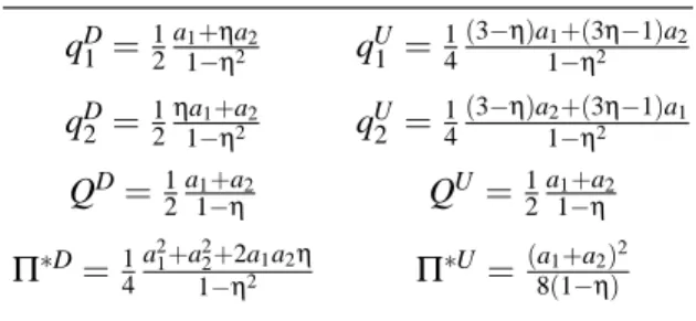
Price Discrimination Uniform price qD1 =12a1+ηa2 1−η2 qU1 =14 (3−η)a1+(3η−1)a2 1−η2 qD2 =12ηa1+a2 1−η2 qU2 = 1 4 (3−η)a2+(3η−1)a1 1−η2 QD=12a1+a2 1−η QU=12 a1+a2 1−η Π∗D=1 4 a21+a22+2a1a2η 1−η2 Π ∗U=(a1+a2)2 8(1−η)
Table 4: Price Discrimination and Uniform prices
But the increment in consumer surplus is different. We use the fact that total quantity is the same in both regimes: ∆CS=CS(qD1,qD2)−CS(qU1,qU2) = 1 2 qD1 2 +12 qD22−ηqD1qD2 −12 qU12+12 qU22−ηqU1qU2 = =12 qD1 +qD22−(1+η)qD1qD2 −1 2 q U 1 +qU2 2 −(1+η)qU1qU2= = (qU1qU2 −qD1qD2)(1+η).
It is easy to chech that
∆CS= (1+η) (3−η)a1+(3η−1)a2 4(1−η2) (3−η)a2+(3η−1)a1 4(1−η2) − a1+ηa2 2(1−η2)η a1+a2 2(1−η2) =−3 16 (a2−a1)2 1+η .
And the total change in welfare is:
∆W =∆Π+∆CS=1 8 (a2−a1)2 1+η − 3 16 (a2−a1)2 1+η =− 1 16 (a2−a1)2 1+η .
So, total output remains the same with third-degree price discrimination, but welfare does not increase; moreover, it is reduced. And Proposition 3 by Adachi is no longer true. It is easy to verify that if we measure consumer surplus as Adachi, CSA(q1,q2) =21(q21+q22), we get the Adachi’s results.
References
[1] Adachi T., 2002, A Note on Third-Degree Price Discrimination with Interdependent Demands, Journal of Industrial Economics, 50, 235 (forthcoming at the Journal of Industrial Economics (JIE) Notes and Comments page: http://www.stern.nyu.edu/ jindec/notes.htm)
[2] Armstrong, M. and J. Vickers, 2001, Competitive price discrimination, RAND Journal of Economics, 32, 579-605.
[3] Layson, Stephen K., 1994, Third-Degree Price Discrimination under Economies of Scale, Southern Economic Journal, 61, 323-327.
[4] Schmalensee, R., 1981, Output and Welfare Implications of Monopolistic Third-Degree Price Discrim-ination, American Economic Review, 71, 242-247.
[5] Schwartz, M., 1990, Third-Degree Price Discrimination and Output: Generalizing a Welfare Result, American Economic Review, 80, 1259-1262.
[6] Stole, L., 2001, Price Discrimination in Competitive Environments, (preliminary and incomplete), prepared for the Handbook of Industrial Organization, (version November 7, 2001) It can be reached at: “http://gsblas.uchicago.edu/Lars Stole.html”
[7] Varian, H. R., 1985, Price Discrimination and Social Welfare, American Economic Review, 75, 870-875.