ADEMU WORKING PAPER SERIES
Generalized Compensation Principle
Aleh Tsyvinskiƚ Nicolas Werquinŧ July 2018 WP 2018/137 www.ademu-project.eu/publications/working-papers
Abstract
We generalize the classic concept of compensating variation and the welfare compensation principle to a general equilibrium environment with distortionary taxes. We derive in closed-form the solution to the problem of designing a tax reform that compensates the welfare gains and losses induced by an arbitrary economic disruption. In partial equilibrium, average taxes simply increase or decrease to counteract the revenue gains or losses caused by the disruption. In general equilibrium, the compensation features three elements that depart from this benchmark and respectively account for (i) the incidence of the initial exogenous shock, and the fact that the tax reform itself induces indirect welfare effects caused by (ii) the non-constant marginal product of labor and (iii) the skill complementarities in production. This leads to a progressive compensating tax reform, with average tax rates increasing at a rate given by the ratio of the elasticity of labor demand and the elasticity of labor supply net of the rate of progressivity of the pre-existing tax code. We also derive a closed form formula for the fiscal surplus of the wage disruption and the compensation, thus generalizing the traditional Kaldor-Hicks criterion. Finally, we apply our formula to the compensation of automation: in the U.S., one additional robot per thousand workers requires a reduction (resp., increase) in the average tax rate at the 10th (resp., 90th) percentile of the income distribution equal to 2 percentage points (resp., 0.5 pp).
Keywords: income taxation, compensation principle, general equilibrium, wage disruption, robots
Jel codes: E62, H21, H22, I38
ƚ Yale University
Acknowledgments
We thank Andy Atkeson, Don Brown, Ariel Burstein, Raj Chetty, Wolfgang Dauth, Georgy Gorov, Eduardo Faingold, Axelle Ferriere, Sebastian Findeisen, Jim Hines, Marek Kapicka, Louis Kaplow, Rohan Kekre, Nicolas Lambert, Tim Lee, Jesse Perla, Pascual Restrepo, Stefanie Stantcheva, Christopher Tonetti, Gianluca Violante, Dominik Sachs, and Kjetil Storesletten for comments. This research has received financial support from the ADEMU network grant, part of the EU H2020 program (grant agreement No 649396).
_________________________
The ADEMU Working Paper Series is being supported by the European Commission Horizon 2020 European Union funding for Research & Innovation, grant agreement No 649396.
This is an Open Access article distributed under the terms of the Creative Commons Attribution License Creative Commons Attribution 4.0 International, which permits unrestricted use, distribution and reproduction in any medium provided that the original work is properly attributed.
Introduction
In this paper we generalize the classic concept of compensating variation and the welfare compensation principle to a general equilibrium environment in which only distortionary taxes are available.
Consider a disruption in the economy, for example, an inow of immigration or a change in technology, that impacts the distribution of workers' wages. This economic shock generally creates winners and losers, i.e., welfare gains for some individuals and welfare losses for others. The welfare compensation problem consists of designing a reform of the tax-and-transfer system that osets these losses by redistributing the gains of the winners. The traditional public nance literature (Kaldor [1939], Hicks [1939,1940]) gives a straightforward answer to the welfare compensation problem. In an economy where type-dependent lump-sum taxes are available, the tax reform that redistributes the welfare gains and losses from the economic shock simply consists of raising (resp., lowering) in a lump-sum way the tax liability of agents whose welfare increases (resp., decreases) from the disruption, up to the point where everyone is exactly as well o as before the change. This standard Kaldor-Hicks approach is awed, however. First, because of asymmetric information, the only tax instrument at the disposal of the government, the income tax, is distortionary (Mirrlees[1971]), so that agents' labor supplies adjust in response to the tax change. Second, we argue that it is important to design the tax reform in an environment that explicitly accounts for the fact that wages are endogenously determined in general equilibrium. Consider for example an immigration inow, i.e., an exogenous (relative) increase in the total labor supply of a given skill. This disruption lowers the wage of agents with the same skill because the marginal product of labor is decreasing and raises the wage of those whose skills are complementary in production. In this situation, therefore, it is clear that immigration ows have non-trivial welfare consequences only because of the general equilibrium forces. Similarly, the impact of automation on inequality can be understood as a race between education and technology, whereby movements in relative wages are driven by the changes in the relative supply and demand of skills. Now suppose that the government implements a tax reform that aims at compensating the welfare of agents whose wage is adversely impacted by the disruption. Since the only available policy tools are distortionary taxes, such a reform aects the agents' labor supply choices. By the same general equilibrium forces as we
just described, these labor supply adjustments impact in turn individuals' wages, and hence their utility. These welfare implications need to be themselves compensated using the distortionary tax code, leading to an a priori complex xed point problem. We start by analyzing the welfare compensation problem in a partial equilibrium environment where wages are exogenous. We show that the design of the compen-sating tax reform which brings every agent's utility back to its pre-disruption level is simple, even when only distortionary taxes are available. The key insight here is that individual utility is only aected by the average tax rates of the reform that is, the changes in marginal tax rates do not impact welfare. This follows from an envelope theorem argument: the marginal tax rate that the individual faces aects his indirect utility only through his optimal labor supply decision, so that the cor-responding welfare eect is second-order. As a consequence, it is straightforward to show (Proposition 1) that a suitably designed adjustment in the average tax rate namely, one that exactly cancels out the income gain or loss caused by the exogenous disruption is sucient to achieve welfare compensation.
The analysis becomes signicantly more complicated when distortionary taxes are coupled with the general equilibrium considerations. In this case, despite the envelope theorem, the endogenous changes in labor supply do matter for welfare, through their impact on wages that result from the decreasing returns and the complementarities in production. Therefore, in general equilibrium, because of the labor supply responses it generates, the marginal rates of the tax reform aect directly the agent's utility, even conditional on the average tax rate change. In other words, to determine the compensating tax reform, we need to simultaneously solve for the average and the marginal tax rate functions. This is the key dierence with the partial equilibrium environment and the main technical challenge of our paper.
The main result of our paper is Theorem 1 that gives a closed-form solution and thus provides the complete analytical characterization of the compensating tax reform in response to any wage disruption in general equilibrium. This formula is valid for marginal wage disruptions; that is, our tax reform compensates the rst-order eects on welfare caused by this shock. Corollary 2 also derives a closed-form formula for the scal surplus of the wage disruption and its compensation, i.e. the impact on government budget of the disruption and its associated compensation, which generalizes the traditional Kaldor-Hicks criterion and provides a simple test to determine whether economic shocks or policies are benecial, in the sense that
oseting their associated individual welfare gains and losses using only distortionary tax instruments is budget-feasible.
For ease of exposition, our theoretical analysis proceeds in two steps. We rst analyze a simplied version of our model in Section 1, in which we make a num-ber of assumptions ensuring that all of the relevant elasticity variables are constant. Specically, we assume there that the utility function is quasilinear with isoelastic disutility of labor, that there are no labor force participation decisions, that the pro-duction function has a constant elasticity of substitution (CES) over labor inputs, and that the tax schedule in the initial (undisrupted) economy has a constant rate of progressivity. These functional-form assumptions allow us to derive in the simplest possible way the welfare compensating tax reform and analyze its economic implica-tions. Second, in Section 2, we relax all of these assumptions: we allow for general individual-specic preferences with income eects, intensive (hours) and extensive (participation) labor supply decisions, a general production function over the labor inputs of all skills and capital, and an arbitrarily non-linear initial tax schedule. We derive a closed-form solution to the compensation problem in this environment that directly generalizes that obtained in the simpler framework.
Our theoretical analysis shows that there are three key elements, all given in closed-form, in the formula for the welfare compensating tax reform that depart from the simple partial equilibrium policy. First, the modied wage disruption variable properly denes the relevant disruption that needs to be compensated namely, one that accounts for all of the labor demand spillovers induced by the initial shock.
Second, the progressivity variable accounts for the fact that a reform of the marginal tax rate of an agent distorts his labor supply, which in general equilib-rium aects his wage because the marginal product of labor is decreasing. Therefore, the compensation needs to be designed in such a way that the welfare eects caused indirectly by the marginal tax rates of the reform counteract those induced by the average tax rates. This naturally leads to a dierential equation for the compensa-tion, and hence exponentially decreasing or increasing income tax rates. This implies, in response to a positive (resp., negative) disruption of a given wage, a progressive (resp., regressive) tax reform on incomes below that of the disrupted agent. The rate of progressivity is determined by the ratio of the labor supply and labor demand elasticities, net of the rate of progressivity of the initial tax code.
lower marginal tax rate at a given income, by distorting labor supply, also aects the entire wage distribution because of the cross-wage eects originating from the skill complementarities in production. The welfare impact of this indirect wage adjust-ments needs to be itself compensated using the tax schedule. However, the marginal tax rates of this second round of compensation generate in turn further wage and welfare changes for all of the agents, and so on. This leads to an a priori complex sequence of compensations formally represented by an integro-dierential equation. We show that we can generally solve this xed point problem in closed-form by den-ing inductively a sequence of functions that each capture a given round of iterated compensation. Remarkably, if the production function is CES, we show that each round of iterated compensation is a constant fraction of the previous one. In this case, compensating the welfare gains and losses resulting from the skill complemen-tarities in production simply requires a uniform shift of the marginal tax rates in addition to the progressive reform derived in the absence of cross-wage eects.
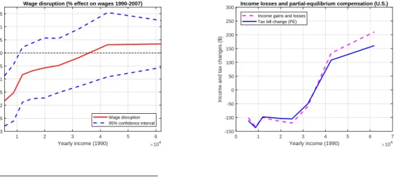
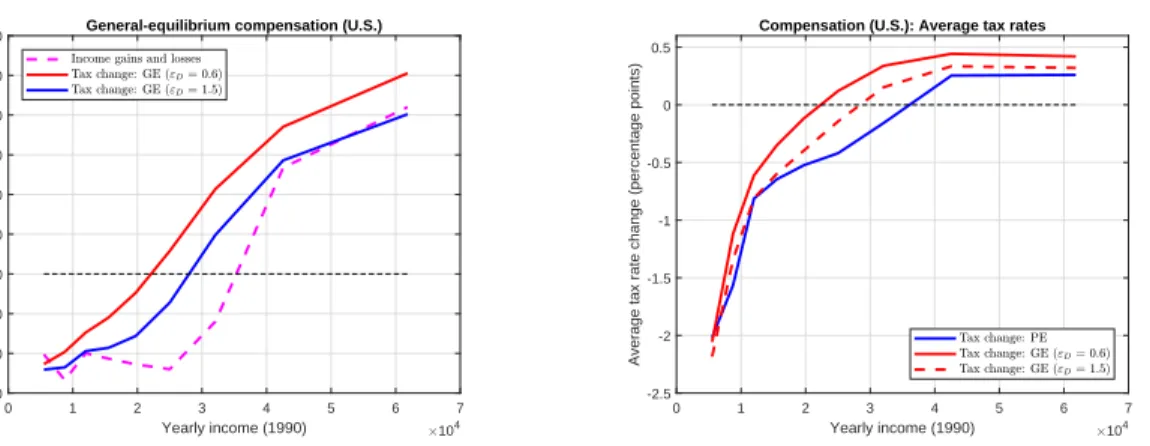
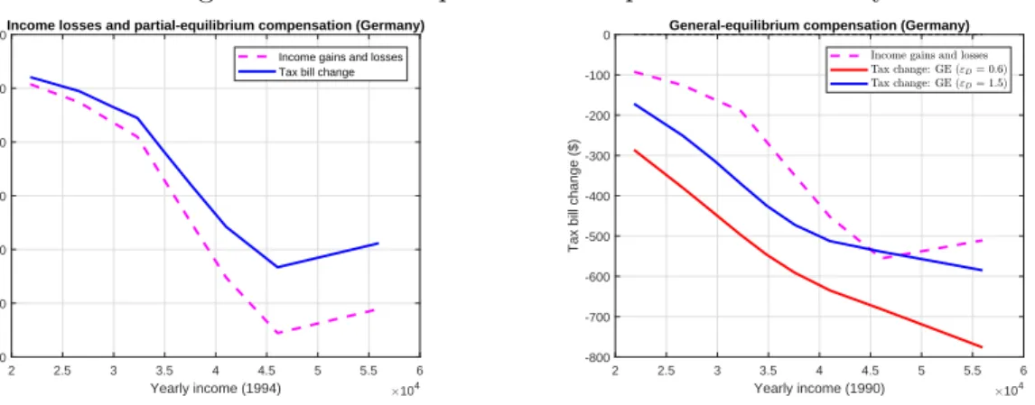
We nally propose in Section 3a concrete application of our theory in the context of the robotization of the U.S. and the German economies between 1990 and 2007. We use Acemoglu and Restrepo [2017]'s data for the U.S., and Dauth et al (2017) data for Germany, which give the estimated impact of an additional robot per one thousand workers on the wages of dierent skills roughly the amount of automation observed in the U.S. between these dates. The closed-form solution that we derive allows to immediately determine quantitatively the compensating reform. We nd that in the U.S., an additional robot per thousand workers requires a progressive tax reform, where the tax payment of agents at the 10th (resp., 90th) percentile of the wage distribution decreases (resp., increases) by 110% of their income loss (resp., 125% of their income gain) from the disruption. This represents a 2 percentage point decrease (resp., a 0.5 pp increase) in their average tax rate, and generates a positive $16 budget surplus for the government. In Germany, workers at the 10th percentile should have their tax bill reduced by 310% of their income loss, while those at the 90th percentile should have theirs reduced by 150% of their income loss.
Related literature. We now briey describe the relationship to the literature. There are two main (and closely related) approaches in the theory of taxation. The rst, represented by Saez and Stantcheva [2016], consists of assuming a particular social welfare function, or more generally of choosing the generalized social welfare
weights that society assigns to dierent agents, and deriving optimal taxes given this criterion. The second approach, analyzed byKaplow[2012,2004] andHendren[2014], consists of generalizing the Kaldor-Hicks principle in the partial equilibrium setting. Our results in Section1.4, which consist of constructing the compensating tax reform in partial equilibrium, build on their work. Our main contribution (in particular, Proposition2and Theorem1) is the analysis of the general equilibrium environment, where a disruption to the wage of an agent and a tax reform also directly impact the welfare of other individuals. We discuss the advantages of the compensation approach for the eld of taxation in Section A.6.
Second, and most closely related to our general equilibrium framework, Itskhoki [2008] and Antras, de Gortari, and Itskhoki [2016] study compensating tax reforms and the welfare implications of trade liberalization in a general-equilibrium setting within a class of distortionary taxes. Itskhoki [2008] solves for optimal redistribu-tion in a closed and open economy following trade liberalizaredistribu-tion within a class of distortionary taxes. Antras, de Gortari, and Itskhoki [2016] solve for the welfare and inequality correction following trade liberalization, restricting taxes (as well as tax reforms) to be of the CRP form (Bénabou [2002], Heathcote, Storesletten, and Violante [2016], Heathcote, Storesletten, Violante, et al. [2017]) and the production function to be CES. While we do not consider a sophisticated model of trade, we solve the compensation problem allowing for both general nonlinear tax schedules and tax reforms, and a general production function. More broadly, our model is within the class of Mirrleesean economies in general equilibrium. Stiglitz[1982a],Rothschild and Scheuer [2013, 2014, 2016], Ales, Kurnaz, and Sleet [2015a,b], Scheuer and Werning [2016],Sachs, Tsyvinski, and Werquin[2016] study optimal taxes in this environment. These papers do not address the compensation problem, which is our main contribu-tion and leads to dierent economic insights, as well as a simpler implementacontribu-tion in practice (since it is known in closed-form).
Third, our application to automation relies on the results of Acemoglu and Re-strepo [2017] (for the U.S.) and Dauth, Findeisen, Südekum, and Woessner [2017] (for Germany), who estimate the impact of robots on the wage distribution.
1 A Simple Model
We start by presenting a very simple version of our general framework, which allows us to derive most transparently our main result namely, a closed-form formula for the tax reform that osets the welfare gains and losses of an arbitrary disruption of the wage distribution in general equilibrium. Specically, we make in this section the following assumptions: (i) the utility function is quasilinear with an isoelastic disutility of labor eort, and is the same for all agents; (ii) labor supply is chosen on the intensive margin only, i.e., there are no participation decisions; (iii) the production function has a constant elasticity of substitution (CES) over the labor inputs of all skill types, and there is no capital input; (iv) the labor income tax schedule in the initial (undisrupted) economy has a constant rate of progressivity (CRP). (Note, however, that we allow tax reforms to be arbitrary nonlinear functions of labor income.) The goal of these assumptions is to ensure that the relevant behavioral and price elasticities are constant.1 We relax them and solve the fully general model in Section2.
1.1 Initial equilibrium
There is a continuum of measure one of individuals indexed by i ∈ [0,1]. In this
section, we assume for simplicity that all agents have quasilinear preferences over consumptioncand labor supplyl with isoelastic disutility of eort: u(c, l) = c−l1+ 1e
1+1e. Agent i earns a wage wi ∈ R+ which he takes as given. He chooses his labor supply
li and earns pre-tax labor income yi = wili. He pays a tax T (yi) on labor income, where the non-linear tax schedule T : R+ → R is twice continuously dierentiable. Agenti maximizes his utility subject to the budget constraintc=wil−T(wil). The agent's indirect utility is given by
Ui = wili−T (wili)− l1+ 1 e i 1 + 1e, (1)
1Specically, Assumptions (i) and (ii) imply that the agents' elasticities of labor supply with
respect to the marginal tax rate are constant, and that the income eects and the elasticities of participation are equal to zero. Assumption (iii) implies that the elasticities of labor demand with respect to the wage are constant, as well as the cross-wage elasticities with respect to the labor supply of a given skill, that is, an agent's labor supply has the same percentage impact on the wage of all other workers. Assumption (iv) ensures that the labor supply elasticities with respect to the wage, as well as the indirect adjustments of labor supply due to the agents' endogenous movements along the nonlinear tax schedule, are constant.
where his labor supply li is characterized by the rst-order condition
li = [(1−T0(wili)) wi] e
. (2)
We denote by w ≡ {wi}i∈[0,1], l ≡ {li}i∈[0,1], U ≡ {Ui}i∈[0,1] and L ≡ {Li}i∈[0,1] the distributions of individual wages, labor supplies, indirect utilities and aggregate labor supplies in the initial economy with tax schedule T. Without loss of generality, we can order agents so that wages wi are increasing in the indexi, given the initial tax schedule T. Hence the agent's skill type i can be interpreted as his percentile in the wage distribution in the initial (undisrupted) economy.2
There is a continuum of mass one of identical rms that produce output using the aggregate labor supply3 L
i of each type i∈ [0,1]. In this section, we assume for simplicity that the aggregate production function has a CES functional form (as in, e.g., Heathcote et al. [2016]):
F({Li}i∈[0,1]) = ˆ 1 0 θiL 1− 1 εD i di εDεD−1 , (3)
whereθi >0for alli. The parameter εD >0is the constant elasticity of substitution between any two labor inputs. If εD → ∞, the environment converges to the partial
equilibrium model where wages are exogenous and given by wi = θi for all i.4 In equilibrium, rms earn no prots, and the wage wi is equal to the marginal product of type-i labor: wi = Fi0(L) = θi ¯ Y Li 1/εD , (4) where F0
i ≡ ∂F/∂Li denotes the partial derivative of F with respect to its ith
2Using (2) and (5), it is then easy to show that incomesy
i =wili are then strictly increasing in
skillsi, so that there are one-to-one maps between skills, wages and incomes in the initial equilibrium.
Importantly, we do not require that the tax reforms we consider keep this monotonicity property.
We assume that incomesy belong to a compact interval[y,y¯]⊂R+ and have a continuous density
fY (·).
3Since the distribution of agents on [0,1] is uniform, we have Li = li in equilibrium. Note,
however, that each individual agent is atomistic within his skill group, so that his wage changes only if all individuals with the same skill adjust their labor supply (e.g., in response to a tax change). In particular, each agent takes his wage as given and independent of his own choices.
4IfεD = 1 (resp.,εD →0), the production function is Cobb-Douglas (resp., Leontie). Labor
variable Li and Y¯ ≡F(L)is the average income in the economy.
The government levies taxes on labor income. In this section, we assume for simplicity that in the initial equilibrium, i.e. before the disruption occurs, the tax schedule has a CRP functional form:5
T(y) = y− 1−τ
1−py
1−p
, (5)
with p∈ (−∞,1) and τ ∈ R. The parameter p is the constant rate of progressivity of the tax schedule, dened as (minus) the elasticity of the retention rate(1−T0(y))
with respect to gross income y. In particular, if p = 0 (resp., p > 0, p < 0) the
initial tax schedule is linear (resp., progressive, regressive). Importantly, we allow the government to implement arbitrarily nonlinear reforms (i.e., not necessarily in the CRP class) in response to a given wage disruption.
1.2 Wage disruptions and the welfare compensation problem
In this section we start by dening a disruption of the economy's initial equilibrium, and then formally set up the welfare compensation problem. A disruption can be caused by various exogenous shocks: e.g., a perturbation of the production function
F (due to, say, technological change) or of the distribution of aggregate labor supplies
L={Lj}j∈[0,1] (due to, say, immigration ows).6 Suppose that this shock aects the wage distribution w by µwˆE = {µwˆE
i }i∈[0,1] for some µ > 0, so that the wage of agent i ∈ [0,1] changes from wi to wi + µwˆEi . The disruptions we consider are continuous maps i 7→ µwˆiE on [0,1], and without loss of generality we normalize
kwˆEk ≡ max
i∈[0,1]|wˆ E
i | = 1. The function wˆ
E thus denes the direction of the wage disruption, while the scalar µrepresents its size.
Denition 1. (Wage disruption.) Consider an exogenous shock ( ˆFE,LˆE) to the
economy's production functionF and the initial equilibrium distribution of aggregate labor supplies L. We dene the wage disruption µwˆE, with kwˆEk = 1 and µ > 0,
by the change in the wage distribution w caused by these shocks, keeping individual
labor supplies xed: for all i ∈ [0,1], µwˆE i = ˜F 0 i({Lj + ˆLEj}j∈[0,1])−F 0 i({Lj}j∈[0,1]), where F˜ ≡F + ˆFE.
5See, e.g.,Bénabou[2002], Heathcote, Storesletten, and Violante[2016].
6In Section 2, where capital is an input in production, a disruption can also be caused by an
The government can implement an arbitrarily nonlinear tax reform µTˆ(·) of the
tax schedule,7 so that the statutory tax payment at income levelychanges fromT (y)
toT (y) +µTˆ(y).
In response to a wage disruption µwˆE and a tax reformµTˆ, individuals optimally adjust their labor supply. In general equilibrium, this further impacts their wage, which in turn alters their labor supply decisions, and so on. We denote by µwˆi and
µˆli the total endogenous changes in individuali's wage and labor supply following the perturbation(µwˆE, µTˆ). That is, the wage and labor supply of an agent with skilliin the equilibrium of the disrupted economy are respectively equal tow˜i =wi+µwˆiE+µwˆi and ˜li =li +µˆli. We denote by U˜i = Ui+µUˆi the resulting indirect utility of agent
i in the new equilibrium. Formally, the agent's welfare in the disrupted economy is given by ˜ Ui = w˜i˜li−T( ˜wil˜i)−µTˆ( ˜wi˜li)− ˜ l1+ 1 e i 1 + 1e, (6)
where ( ˜wi,˜li) are dened by the perturbed rst-order condition
˜
li = [(1−T0( ˜wi˜li)−µTˆ0( ˜wi˜li)) ˜wi]e, (7) and the perturbed wage equation
˜
wi = F˜i0({L˜j}j∈[0,1]). (8) with L˜j ≡Lj + ˆLE
j +µˆlj.
A wage disruption µwˆE generally creates winners and losers, i.e., welfare gains
for some individuals and welfare losses for others. The welfare compensation problem consists of designing a reform Tˆ of the existing tax code that osets these losses by
redistributing the income gains of the winners. Such a tax reform must be designed
7In Section 1.5 we assume that the tax reforms Tˆ that the government can implement are
continuously dierentiable, bounded, with bounded rst derivative. This denes a Banach space on
which the norm of a functionTˆ is given by kTˆk= sup
y∈R+
|Tˆ(y)|+ sup y∈R+
|Tˆ0(y)|. Note that we do not
imposekTˆk= 1, so that the normalization of the tax reform by the same scalar µ >0 as the wage
disruption is without loss of generality. The same holds for the endogenous wage and labor supply adjustmentsµwˆi, µˆli below.
such that each agent's compensating variation8 U˜i−Ui is equal to zero, taking into
account the endogenous wage and labor supply responses that it induces.
Denition 2. (Welfare compensation problem.) A welfare compensating policy in response to a wage disruption µwˆE is a tax reform µTˆ such that: (i) the utility
˜
Ui of each agent i after the disruption, dened in (6), and the tax reform satises
˜
Ui = Ui; (ii) labor supply is chosen optimally, i.e. (7) holds; and (iii) the wage is equal to the marginal product of labor, i.e. (8) holds. Equation (41) in the Appendix denes the scal surplus, i.e., the change in government revenue induced by the wage disruption µwˆE and the compensating tax reform µTˆ.
In what follows, we characterize analytically the solution to the welfare compen-sation problem for marginal wage disruptions, i.e., as µ → 0. Thus, our exercise
consists of designing a tax reform Tˆ that compensates the rst-order welfare eects
of a small wage disruption in the direction wˆE.
1.3 Elasticity concepts
We rst dene the elasticities εS,ri and εS,wi of labor supply li with respect to the retention rate ri ≡ 1−T0(wili) and the wage wi respectively, along the nonlinear budget constraint, as9 εS,ri ≡ ∂lnli ∂lnri = e 1 +pe, and ε S,w i ≡ ∂lnli ∂lnwi = (1−p)e 1 +pe . (9)
The (constant) labor supply elasticityεS,r diers from the structural parametereas it takes into account that the initial labor supply response to a change in the retention rate impacts the marginal tax rate T0(wili) faced by the agent, if the initial tax schedule is nonlinear, by an amount equal to the rate of progressivitypof the nonlinear tax schedule; this in turn causes a further endogenous labor supply adjustment given by the elasticity e, leading to the correction term p×e in the denominator of εS,r. Moreover, the elasticity with respect to the wage, εS,w, diers from that with respect
8See, e.g.,Mas-Colell, Whinston, and Green[1995], p. 82. Since the utility function is quasilinear,
it is the monetary amount that an agenti would be willing to pay, after the wage disruptionµwˆE
and the tax reform µTˆ, in order to be as well o as in the initial equilibrium. A positive (resp.,
negative) value implies that an individualibenets (resp., loses) from these shocks.
9The assumptions we made in Section1.1 ensure that the these elasticities are constant. This
to the retention rate,εS,r, because a change in the wage aects(1−T0(w
ili))wi, and hence labor supply, both directly as in the case of an exogenous perturbation in the retention rate, and indirectly through its eect on the marginal tax rate T0(wili). The latter is accounted for by the correction (1−p)in the numerator of εS,w.
Second, we dene the elasticities of wages{wi}i∈[0,1] with respect to the aggregate labor supply Lj. The labor supply of type j aects the wage of any other skill i6=j because dierent skills are imperfect substitutes in production, and the wage of skill j because the marginal product of labor is decreasing. We dene the corresponding structural cross-wage and own-wage elasticities γi,j and 1/εDj , respectively, by
γi,j ≡ ∂lnwi ∂lnLj = 1 εD yj ¯ Y , and 1 εD j ≡ −[∂lnwj ∂lnLj −lim i→j ∂lnwi ∂lnLj ] = 1 εD (10)
where both equalities are proved in the Appendix. The rst expression shows that when the production function is CES, the cross-wage elasticity γi,j ≡ ∂∂lnlnwLji does not depend on i, implying that a change in the labor supply of type j has the same percentage impact on the wage of every type i6=j; for the remainder of this section we thus simply denote γi,j by γj. The second expression constructs the own-wage elasticity1/εDj , or equivalently the inverse of the partial-equilibrium elasticity of labor demand, by subtracting from ∂lnwj
∂lnLj the complementaritylimi→j
∂lnwi
∂lnLj between skillj and
its neighboring skills i ≈ j, thus capturing the impact of the labor eort Lj on the wage wj arising purely from the fact that the marginal productivity of skill j is a decreasing function of the aggregate labor of its own type. With a CES production function with parameter εD, this elasticity is constant and equal to 1/εD.
1.4 Compensation in Partial Equilibrium
In this section, we show that the solution to the compensation problem takes a simple form in partial equilibrium, even when when taxes are distortionary. Suppose that there is innite substitutability between skills in production, i.e., εD → ∞. The
production function thus reads F(L) = ´01θiLidi, so that wages are exogenous and equal towi =θifor alliin the initial equilibrium.10,11In this case, the wage disruption
µwˆE generates no further endogenous adjustment in the wage: wˆi = 0for alli∈[0,1],
10This is the standard partial-equilibrium assumption made byMirrlees[1971].
11As will be clear in Section2.4, none of the results of this section (except formula (12)) rely on
so that w˜i is simply equal to wi +µwˆEi . We characterize analytically the solution to the welfare compensation problem, i.e., the compensating tax reform µTˆ and its scal surplusµR( ˆwE), for marginal wage disruptions. The proofs are gathered in the
Appendix.
A rst-order Taylor expansion of equation (6) around the initial equilibrium (i.e., asµ→0) implies that the changeUˆi in the indirect utility of agent iinduced by the wage disruption and the tax reform is given by:
0 = Uˆi = (1−T0(yi))yi
ˆ
wiE wi
−Tˆ(yi), (11) where the rst equality imposes that agent i keeps the same level of welfare in the disrupted economy as in the initial equilibrium (i.e., U˜
i = Ui), once the new tax schedule is implemented. This equation shows that, in the partial equilibrium model, the change in the indirect utility of agent i is due to: (i) the exogenous change (say, increase) wˆiE in his wage, weighted by the share (1−T0(yi)) that he keeps after paying taxes on the implied income gainliwˆEi =
yi
wiwˆ
E
i (the rst term of (11)); (ii) the change in his tax liability Tˆ(yi) (the second term of (11)), which makes him poorer
(resp. richer) if Tˆ(yi)>0(resp. <0).
Crucially, note that the change in the marginal tax rate, Tˆ0(y
i), does not enter equation (11), and therefore does not matter for welfare (conditional on the average tax rate Tˆ(y
i)). This follows from the envelope theorem: the marginal tax rate that individuals face aect agents' indirect utility only through their labor supply decision (equation (2)); but since they choose labor supply optimally before the perturbation, their behavioral response to the marginal tax rate change induces no rst-order eect on welfare.12
Next, a rst-order Taylor expansion of equation (6), which imposes that the labor supply of agent i remains optimal in the disrupted economy, can be written in terms of the elasticity notations introduced in Section 1.1 as:
ˆ lpei li = εS,w wˆ E i wi −εS,r ˆ T0(yi) 1−T0(y i) . (12)
This equation shows that the agent's labor supply adjusts because of the change in his wage wˆE
i , by an amount given by the labor supply elasticity with respect to the
wageεS,w, and the change in his marginal tax rateTˆ0(y
i), by an amount given by the elasticity with respect to the retention rate εS,r.
We now summarize the results obtained so far. Equation (11) immediately gives the tax reform µTˆ which ensures that, after reoptimizing their behavior, individuals remain as well o as before the wage disruption µwˆE. Equation (12) gives the
cor-responding change in the labor supply of agents following this wage disruption and compensating tax reform, and the impact on government budget is then straightfor-ward to derive. We thus obtained the solution to the welfare compensation problem in closed form.
Proposition 1. Suppose that there is innite substitutability between skills in pro-duction, i.e., εD → ∞. Consider a marginal disruption of the wage distribution w in the direction wˆE ={wˆE
i }i∈[0,1]. There exists a unique tax reform Tˆ that solves the welfare compensation problem, namely: for all i∈[0,1],
ˆ T (yi) = (1−T0(yi))yi ˆ wE i wi . (13)
The scal surplus R( ˆwE) is given by expression (42) in the Appendix.
Proposition 1is our rst step in generalizing the standard Kaldor-Hicks criterion to the environment where type-specic lump-sum taxes are unavailable. It shows that if wages are exogenous, the compensating tax reform consists of increasing or decreasing the average tax rates Tˆ(yi)
yi by an amount equal to the net-of-tax income
gain or loss of agents resulting from the economy's disruption, (1−T0(yi)) ˆ wE
i
wi.
1.5 Compensation in General Equilibrium
In this section we analyze the welfare compensation problem in the general equi-librium environment, that is, for any εD > 0. We show in the Appendix that the mathematical structure of this problem is a system of integro-dierential algebraic equations (IDAE). We derive its solution in a closed-form for marginal wage disrup-tions, i.e., to a rst-order as the size of the shock µ→0. The proofs are gathered in
the Appendix.
As discussed in Section1.2, in general equilibrium, the initial wage disruptionµwˆE
agent's indirect utility and choice of labor supply. A rst-order Taylor expansion of equation (8) implies that the endogenous wage changes wˆi are given by
ˆ wi wi = − 1 εD ˆ li li + ˆ 1 0 γj ˆ lj lj dj, (14)
where 1/εD andγj are respectively the own-wage and cross-wage elasticities, dened in (10). This equation has the following economic interpretation: a one percent increase in the labor supply of an individual with skill i leads to a −1/εD percent change in the wage of type i, because the marginal product of labor is decreasing; analogously, a one percent increase in the labor supply of an individual of type j, for any j ∈ [0,1], leads to a γj percent change in the wage of type i, through the complementarities between skills in production.
Now, following the same steps as in Section 1.4, a rst-order Taylor expansion of equation (6) around the initial equilibrium implies that the change Uˆ
i in the indirect utility of agent i induced by the wage disruption and the tax reform is given by:
0 = Uˆi = (1−T0(yi))yi ˆ wEi wi +wˆi wi −Tˆ(yi), (15) where the rst equality imposes that agent i keeps the same level of welfare in the disrupted economy as in the initial equilibrium. This expression generalizes equation (11) (replacing wˆEi with wˆEi + ˆwi) and implies that, in addition to the two partial-equilibrium forces described in Section 1.4, there is now the third channel through which the compensating variation of the agent changes, namely: (iii) the endogenous changesˆliand{ˆlj}j∈[0,1]in the labor supplies of type-iand type-jagents, by impacting
the wage of skill i by wˆi (through equation (14)), have a rst-order impact on the indirect utility of agent i.
Crucially, despite the envelope theorem, the endogenous changes in labor supply now matter for welfare, through their impact on wages resulting from the decreasing marginal productivities and the complementarities in production. As we demonstrate below, it follows that in general equilibrium and when only distortionary tax instru-ments are available the marginal tax rates of the reform now aect directly the agent's utility through the labor supply responses they induce. This is the key dierence with the partial equilibrium environment.
supply of agent i remains optimal in the disrupted economy, can be written in terms of the elasticity notations introduced in Section 1.1 as:
ˆ li li = εS,w ˆ wEi wi +wˆi wi −εS,r ˆ T0(yi) 1−T0(y i) . (16)
This expression generalizes equation (12) obtained in partial equilibrium (replacing
ˆ
wE
i withwˆEi + ˆwi). The presence of the endogenous wage changewˆi in the right hand side, along with equation (14), implies that, in addition to the direct eects caused by the exogenous wage and tax changeswˆiE and Tˆ0(yi), the adjustment in labor supply of agent i,ˆli, is now also aected by those of all other agents j, {ˆlj}j∈[0,1]. Hence the labor supply changes of all of the agents now have to be solved for simultaneously as functions of the wage disruption function wˆE and the tax reform Tˆ. The following lemma, which follows from Sachs, Tsyvinski, and Werquin [2016], derives the closed-form solution for ˆli, for all i∈[0,1].
Lemma 1. The solution to (16) is given by: for all i,
ˆ li li = δ ˆ lpei li +δεS,w ˆ 1 0 Γj δˆljpe lj dj, (17) where ˆlpe i is dened in (12), δ ≡1/[1 + εS,w εD ], and Γj ≡γj/δ.
Equation (17) shows that the percentage change in the labor supply of typei,ˆli/li, is the sum of two terms. The rst, ˆlpe
i /li, is the partial-equilibrium expression (12), weighted by δ. This weight accounts for the fact that the marginal product of labor is decreasing, so that the agent's initial labor supply adjustment (say, increase) ˆlpe
i lowers his wage by a factor 1/εD, which in turn leads him to reduce his labor supply by a factorεS,w/εD, therefore dampening his initial response byδ ≡1/[1 +εS,w
εD ]. The
second term in (17) accounts for the fact that the wage disruption and the tax reform also lead to percentage increases δˆlpej /lj in the labor supplies of agents of typej 6=i. These responses impact the wage of agent i byΓj(δˆljpe/lj), where Γi =γj/δ can be thought of the total elasticity of the wage of skill i with respect to the labor supply of type j. This total cross-wage elasticity accounts for the direct eect γj, as well as all of the indirect eects occuring in general equilibrium the wage change induces further labor supply responses, which in turn aect wages, etc. When the production function is CES these spillover eects are simply captured by the amplication factor
1/δ.13 Now, this total change in wi implies a change inli given by the elasticity εS,w, again weighted by the factor δ to take into account the decreasing marginal product of labor. Summing over all types j ∈[0,1] leads to equation (17).
Taking stock. We gather and discuss the results obtained so far. In contrast to equation (11) in partial equilibrium, (15) does not yield directly the solution for the compensating tax change Tˆ(y
i) as a function of the exogenous disruption wˆEi . This is because the agent's indirect utility is also aected by the endogenous adjustment in his wage, wˆi, which is determined by the labor supply responses of all agents,
{ˆlj}j∈[0,1], via equation (14). In turn, the labor supply change of any agent j, ˆlj, depends on the changes in the marginal tax rates {Tˆ0(yk)}k∈[0,1] faced by everyone in the economy, via equation (17). Thus, in general equilibrium, both the average and the marginal tax rates of the reform have rst-order welfare repercussions this implies that the consequences of a given tax reform are much richer, and hence the design of the compensating policy much more complex, than in partial equilibrium.
Specically, a higher average tax rate at a given income y∗, Tˆ(y∗) > 0, implies
a reduction in the welfare of agent y∗, by directly making him poorer, as in partial equilibrium (last term in equation (15)). Moreover, in general equilibrium, a higher marginal tax rate at incomey∗, Tˆ0(y∗)>0, implies: (a) a higher average tax rate for
all incomes y > y∗, which reduces the welfare of these agents; (b) an increase in the welfare of agent y∗, who works less (substitution eect, rst term in equation (17)) and hence earns a higher wage (decreasing marginal product, rst term in equation (14)); (c) a decrease in the welfare of all agents y 6= y∗, whose wage decreases due to the lower labor supply of agent y∗ (production complementarities, second term in equation (14)).
Suppose that the planner implements the tax reform (13) that would compensate every agent's welfare in partial equilibrium. Through standard substitution eects, this tax reform aects individual labor supplies and hence, through decreasing returns and complementarities in production, the wage distribution. These lead to additional rst-order welfare eects that need to be themselves compensated, by further re-forming the tax-and-transfer system. Therefore, the combination of distortionary tax instruments and elastic labor supply (whereby marginal tax rates aect labor supply
13This is because each round of indirect general-equilibrium eect on the wage is a constant
behavior) and general equilibrium (whereby labor supply decisions determine wages) leads to a xed point problem for the compensating tax reform. Formally, the tax reform Tˆ is the solution to an integro-dierential equation that we derive in Lemma 3 in the Appendix.
Main result. The next proposition gives a complete analytical characterization of the compensating tax reform in response to any wage disruption in general equilib-rium. Note that since there is a one-to-one map between types i and incomesyi, we can change variables and index by income the wages wyi ≡wi, labor supplieslyi ≡li,
wage disruptions wˆEyi ≡wˆiE, and elasticities γyj ≡γj/y
0(j), Γ
yj ≡Γj/y
0(j).
Proposition 2. Suppose that that the utility function is quasilinear with isoelastic disutility of labor, the production function is CES, and the initial tax schedule is CRP. Consider a marginal disruption of the wage distribution w in the direction wˆE =
{wˆE
i }i∈[0,1]. The following tax reform Tˆ solves the welfare compensation problem: for all i, ˆ T (yi) = (1−T0(yi))yi ˆ y¯ yi Eyi,yj[ ˆΩ E yj +λ]dyj, (18)
where the modied wage disruption variable ΩˆE is dened for all j ∈[0,1]by ˆ ΩEyj ≡ δwˆ E yj wyj +δεS,w ˆ y¯ y Γyk δwˆyE k wyk dyk, (19)
the progressivity variable E is dened by
Eyi,yj ≡ εD δ εS,r 1 yj yi yj εD/εS,r , (20)
and the compensation-of-compensation variable λ is a constant equal to14 E[yj
¯ Y ( ˆΩ E yj− ´y¯ yjEyj,yk ˆ ΩEy kdyk)].
We discuss and interpret formula (18) in Section 1.6. Note that this is a closed-form expression, as it depends only on the exogenous wage disruption wˆE and on
variables that are all observed (or known in closed-form as a function of observables) in
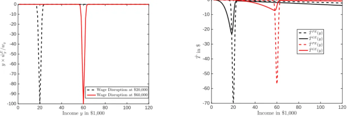
the pre-disruption economy: statutory marginal tax rates, elasticities of labor supply and labor demand, cross-wage elasticity between skills. Therefore it is straightforward to implement such a tax reform in practice.15 In Appendix B.1we provide a graphical
representation and detailed discussion of this formula.
1.6 Analysis of the compensating tax reform
The compensating tax reform (18) features three important departures from the par-tial equilibrium compensation (13).
1. Modied disruption: Accounting for the incidence of the disruption The modied wage disruption ΩˆE
j reects the importance of correctly accounting for the incidence of a given economic shock in general equilibrium. The proof of Proposition 2 shows that ΩˆE
j is equal to the sum of the exogenous and endogenous wage adjustments, δ( ˆwE
j + ˆwj)/wj. Intuitively, (19) shows that for any k the initial shock wˆE
k
wk to the wage of any type k translates into a labor supply response of type
k given by δεS,w wˆEk
wk, which in turn impacts the wage wj of type j by the elasticity Γk. Therefore, the relevant disruption that the tax reform must compensate is ΩˆEj rather than simply wˆjE/wj. Importantly, it is possible that empirical studies that evaluate the impact of a disruption on the wage distribution, capture not only the direct eect of the disruption,{wˆE
j }j∈[0,1], but also all of the indirect eects due to the labor demand spillovers in general equilibrium; this is the case, for instance, in our empirical application in Section 3. In this case, formula (18) can be applied directly using {ΩˆE
j}j∈[0,1] as a primitive.16
2. Progressivity: Accounting for the decreasing marginal product of labor To interpret the progressivity variable (19), we consider a slightly simpler produc-tion funcproduc-tion than (3), with decreasing marginal product of labor but innite substi-tutability between skills: F(L) = ´01θiL
1− 1
εD
i di.17 We can easily show that in this
15See Section3 for an application.
16Conversely, it is also straightforward to derive the exogenous disruption{wˆE
j }j∈[0,1] from the
modied disruption{ΩˆE
j}j∈[0,1].
17This reects, for example, the downward-sloping demand curve for labor when there is a xed
factor of production, such as land or capital, for each type. We assume for simplicity that the government taxes rms' prots at 100%.
case, λ= 0 in formula (18), so that ˆ T (yi) yi = (1−T0(yi)) ˆ y¯ yi Eyi,yjΩˆ E yjdyj, (21) with ΩˆE yj =δwˆ E
yj/wyj. To understand this expression, recall rst that in partial
equi-librium (i.e., asεD → ∞), the tax reform that compensates a disruption{wˆE
i }i∈[0,1]is given by Tˆ(yi) yi = (1−T 0(y i)) ˆ wE yi
wyi. That is, as we discussed in Section1.4, the change in the average tax rate must exactly compensate the exogenous wage disruption, weighted by the retention rate of the initial tax schedule. Now, when the marginal product of labor is decreasing, instead, it is easy to show that equations (15) and (16) imply ˆ T(yi) yi = (1−T0(yi)) δwˆE yi wyi +δε S,r εD Tˆ 0 (yi). (22)
That is, the change in the average tax rate must now compensate both the (modied) wage disruption and, in addition, the wage correction generated endogenously by the marginal tax rate of the reform recall that a change in the marginal tax rate by
ˆ
T0(yi) impacts the labor supply of agents i by δεS,rTˆ0(yi), and hence their wage by δεS,r
εD Tˆ
0(y
i). Solving this dierential equation leads to the solution (21).
Now, consider in particular a disruption that raises the wage of skill i∗ only, i.e. wˆiE∗ > 0 and wˆEi = 0 for all i 6= i∗.18 The partial-equilibrium compensation
ˆ
T (yi) is then equal to zero for all incomes yi 6= yi∗that are not directly disrupted
(i.e. wˆiE = 0). In general equilibrium, instead, equation (22) shows that, for agents
with income yi < yi∗ who are not initially disrupted, the compensating tax reform
must satisfy Tˆ(yi)
yi =
δεS,r
εD Tˆ
0(y
i). In order to raise the tax payment of agent i∗ so as to redistribute his income gain, the government must raise the marginal tax rates on (at least some) incomes yi < yi∗, so that Tˆ0(yi) > 0.19 But this generates a
welfare gain for agent i formally, an increase in the marginal tax rate of agent i byTˆ0(y
i) lowers his labor supply byδεS,rTˆ0(yi) (by construction of the labor supply elasticity), so that his wage increases by 1
εD δε
S,rTˆ0(y
i) (by construction of the labor demand elasticity). This benet needs to be compensated counteracted by a welfare
18Formally, the disruption wˆE
i
wi is a Dirac delta function at skilli
∗.
loss of equal magnitude via an increase in the average tax rate Tˆ(yi)
yi > 0. Thus, the
key insight is that in general equilibrium, the government impacts individual welfare through both the average and the marginal tax rates: an increase in the former (resp., the latter) lowers (resp., raises) the agent's utility. Therefore, a welfare compensating tax reform must be such that these two forces exactly cancel out, so that an agent that incurs a marginal tax rate increase must also incur an average tax rate increase. Crucially, notice that the key parameter is the ratio between the elasticity of labor supply and the elasticity of labor demand, which determines the extent to which an increase in the marginal tax rate raises the agent's welfare by lowering his labor supply (εS,r) and raising his wage (1/εD).
The shape of the compensating tax reform Tˆ depends in particular on whether
εD
δεS,r ≥ 1, or equivalently
εD
εS,r ≥ p, where p is the local rate of progressivity of the
initial tax schedule.20 Suppose rst that εD
δεS,r = 1, i.e., εD εS,r = p. The relationship ˆ T(yi) yi = δεS,r εD Tˆ 0(y
i) then requires that the average and the marginal tax rates of the reform must coincide, so that the compensating tax schedule Tˆ must be linear for
incomes yi ≤ yi∗. More generally, the ratio between the marginal and the average
tax rates must be equal to the constant εD
δεS,r = 1−p+
εD
εS,r, so that the tax reform
that redistributes the wage gain of skill i∗ is given by Tˆ(yi)
yi ∝ y
εD/εS,r−p
i I{yi≤yi∗}. 21
Therefore the tax reform is progressive (resp., linear, regressive) on [y, yi∗), i.e. the
change in the average tax rateTˆ(yi)/yiis increasing (resp., constant, decreasing) with
income, if and only if the ratio of the elasticity of labor demand and the elasticity of labor supply in the initial (undisrupted) economy, εD/εS,r, is larger than the rate of progressivity p of the pre-existing tax code. Empirically, the inequality εεS,rD > pis
clearly satised since we have p≈0.15, εS,r ≈0.3, and εD ≥0.5.22
20This follows from the relationship εD
δεS,r = 1−p+
εD
εS,r, obtained using the denition of δ =
1/[1 +(1−εpD)εS,r].Intuitively, the rate of progressivity of the initial tax schedule matters for the shape
of the compensating tax reform, because if p is higher then a given increase in the marginal tax
rate raises welfare by a larger amount indeed, the wage increase that it induces leads to a smaller
increase in labor supply, as εS,w = (1−p)εS,r. Thus the increase in the marginal tax rate that is
necessary to compensate the welfare impact of a given rise in the average tax rate is smaller.
21Formally, this formula is obtained by letting ΩˆE
yj be a Dirac delta function at yi∗ in formula
(21).
3. Compensation-of-compensation: Accounting for skill complementarities The third novel eect in formula (18), the constantλ, is due to the cross-wage eects originating from the skill complementarities in production. Recall that expression (21) compensates both the individual welfare gains and losses generated by the initial wage disruption, and the own-wage eects induced endogenously by the compensation itself when the marginal product of labor is decreasing. Now, if the government implements this tax reform, a lower marginal tax rate at incomeyj also aects all the other wages {wk}k6=j via the cross-wage elasticities Γyj. The welfare impact of this
indirect wage adjustment needs to be itself compensated using the tax schedule. In turn, the marginal tax rates of this second round of compensation generate further wage and welfare changes for every agent. These again must be compensated, and so on.
Formula (18) shows that when the production function is CES and the labor supply elasticities are constant, this series of compensation-of-compensation takes a strikingly simple form. Formally, the following argument explains why the uniform adjustment λ to the disruption is necessary and sucient to compensate the cross-wage eects induced indirectly by the tax reform. We show in the Appendix that the compensating tax reformTˆsatises the following equation, which generalizes the
formula (21) obtained in the absence of cross-wage eects:
ˆ T(yi) yi = (1−T0(yi)) ˆ y¯ yi Eyi,yj " ˆ ΩEyj −δ ˆ y¯ y Γykδε S,r Tˆ0(yk) 1−T0(y k) dyk # dyj. (23) Indeed, the average tax change at incomeyimust now compensate both the (modied) exogenous wage disruption, as described above, but also the welfare eects induced by the changes in marginal tax rates at incomes {yk}k∈[0,1]. Specically, an increase in the marginal tax rate at income yk by Tˆ0(yk) reduces the labor eort of skill k byδεS,r Tˆ0(yk)
1−T0(y
k), by denition of the labor supply elasticity ε
S,r. This in turn reduces the wage of agent yj by Γyk ×δε
S,r Tˆ0(yk)
1−T0(y
k). Summing over all k ∈ [0,1] leads to the
second term in the square brackets of expression (23). Notice that because of the terms Tˆ0(y
k) in the right hand side, equation (23) is a priori a non-trivial functional equation, and hence does not immediately deliver a closed form solution for the compensating tax reform as opposed to the simpler equation (21). However, since the production function is CES and the labor supply
elasticities are constant, the cross-wage elasticity Γyk depends only on yk, that is, a
change in the labor supply of skill k aects the wage of all the other skills j ∈ [0,1]
by the same percentage amount. But this in turn implies that the marginal tax rate changes {Tˆ0(yk)}k∈[0,1] induce the same welfare eect λ ≡δ
´y¯ y Γykδε
S,r Tˆ0(yk)
1−T0(y
k)dyk on
every agent j ∈ [0,1]. Therefore, the wage changes that must be compensated in
addition to the exogenous disruption are simply a constant. Formula (18) follows immediately; the closed-form expression for λ given in Proposition 2 is obtained by solving the functional equation (23) explicitly.
Assuming for simplicity that y¯ → ∞, the reform derived in (21) must be
com-plemented by the following reform: (1−T0(yi))yi
´∞
yi Eyi,yjλdyj = λ(1−T
0
(yi))yi. This additional compensation consists of a constant change (in percentage terms) in the retention rate of the tax schedule: Tˆ0(y)
1−T0(y) =λ(1−p).23 Therefore, compensating
wage gain by agents with incomey∗ requires a uniform shift of the marginal tax rates in addition to the progressive reform on incomes y < y∗ already characterized in the absence of cross-wage eects.
1.7 Fiscal Surplus and other concepts of compensation
Once we know the compensating tax reform in closed-form, it is straightforward to obtain an expression for the scal surplus Rˆ( ˆwE
) dened in (41), i.e., the budget
impact of the wage disruption and its compensation (Corollary 2 in the Appendix). The welfare gains of the wage disruption wˆE are redistributable if and only if
R( ˆwE)≥0. This, in turn, means that it is possible to use the tax system to obtain a
Pareto improvement.24 More generally than its sign, the value of the scal surplus is
important: it provides a metric that allows to compare, in monetary units, dierent economic shocks. For example, suppose that a given disruption (say, an inow of im-migration) generates more revenue, after implementing the compensating tax reform, than another (say, automation). It follows that the government can achieve a strictly better Pareto improvement from the former shock. s.25 Therefore, Rˆ( ˆwE
) provides
23We can easily show that this is equivalent to an increase in the parameterτ of the baseline tax
scheduleT(y) =y−1−τ
1−py
1−p by an amountτˆgiven by τˆ
1−τ =λ(1−p).
24For instance, the government can redistribute lump-sum the budget surplus, which creates no
distortions since the utility is quasilinear and raises everybody's welfare.
25To see this, consider the best possible redistribution of the tax revenue in case B, sayµBTˆB. By
implementing a tax reform that has the same directionTˆBbut a strictly higher magnitudeµA> µB
as a measure of the benet or cost of a given economic shock.
Finally, it is natural to wonder what the compensating tax reform would be if the government's objective were to compensate every agent so that their welfare would be at least as large (rather than exactly as large) as in the initial economy i.e., such that
˜
Ui ≥ Ui for all i in equation (6). In this case, equation (15) would be an inequality and there would be an obvious multiplicity of solutions to the compensation problem. The rst way to address the issue is to implement the exact compensation (18), and in a second (simultaneous) stage use the extra revenue Rˆ( ˆwE
), if any, to achieve
a Pareto improvement. The second way to address it is to solve the compensation problem by replacing 0 with a given function h(·)in the left hand side of (15), with
h(yi)≥0for alli. That is, we solve the compensation problem by directly specifying the positive welfare improvements that we want to achieve for every skill level. The corresponding compensating tax reform can then be derived following identical steps as in the proof of Proposition2, and its solution would depend directly on the desired function h.
2 The General Model
In this section we relax all of the major assumptions we made in Section1and derive a closed-form generalization of formula (18) for the compensating tax reform.
2.1 Initial equilibrium
Agents dier along two dimensions: their skill i ∈ [0,1], as in Section 1, and their
xed cost of participating in the labor forceκ ∈R+.26 An agent with types (i, κ) has idiosyncratic preferences over consumptioncand labor supplyldescribed byui(c, l)−
κI{l>0}, where the utility function ui is a general, twice continuously dierentiable function that satisesu0i,c >0, u00i,cc≤0,u0i,l, u00i,ll<0, and whereI{l>0} is an indicator function equal to 1 if the agent is employed. If the agent decides to work, he earns a wagewi, chooses his labor supply (hours)li, earns pre-tax labor incomeyi =wili, and
achieves a strictly higher welfare improvement, since the rst-order welfare measures are linear inµ
by construction.
pays a labor income taxT (yi).27 If he decides to stay non-employed, his labor supply is equal to zero and he earns the government-provided transfer −T (0). Finally, he
also owns an exogenous quantity ki of the economy's capital stock, which earns a pre-tax return r.28 Capital income is taxed at the constant rate τ.
The maximization problem of agent (i, κ) reads
Ui,κ ≡ max max l>0 ui(ci(l), l)−κ; ui(ci(0),0) . (24)
whereci(l)is dened by the budget constraint: ci(l) =wil−T(wil) + (1−τ)r ki for any l ≥ 0. Conditional on working, agent (i, κ) chooses labor supplyli that satises the rst-order condition
−u
0
i,l(ci(li), li)
u0i,c(ci(li), li)
= [1−T0(wili)] wi. (25)
We assume thatli is the unique solution to this problem. Moreover, the agent decides to participate if and only if his xed cost of work κ is smaller than a threshold κ∗i, given by
κ∗i = ui[wili−T (wili) + (1−τ) r ki, li]−ui[−T(0) + (1−τ)r ki, 0]. (26) Denote byfi(κ)the density ofκ conditional on skilliand byLi =li
´κ∗ i
0 fi(κ)dκ the total amount of labor supplied by workers of skill i.
Firms produce output using the aggregate labor supply Li of each type i∈ [0,1] and the aggregate capital stock K, which we assume to be in xed supply. The aggregate production function is denoted by F({Li}i∈[0,1] , K). We assume that F has constant returns to scale. In equilibrium, rms earn no prots and the wage wi is equal to the marginal product of type-i labor, i.e.,
wi = Fi0({Lj}j∈[0,1] , K). (27) The equilibrium interest rate is equal to the marginal product of capital, i.e., r =
27As in Section1, we order skills so that there is a one-to-one map between skillsiand wageswi
in the initial equilibrium with tax scheduleT. See AppendixA.2for details.
28We impose that all agents with a given skilli, i.e. a given wage wi, own the same amount of
capital, which ensures that they all choose the same level of labor supply (conditional on working)
F0
K({Lj}j∈[0,1], K).
The government levies taxes on labor and capital incomes. The initial labor income tax schedule is twice continuously dierentiable but is allowed to be arbitrarily nonlinear. We dene the local rate of progressivity of the tax schedule as (minus) the elasticity of the retention rate (1−T0(y)) with respect to gross income y: p(y) =
−∂ln(1−T∂lny0(y)). Finally, we restrict the initial tax schedule and tax reforms on capital
income to be linear.
2.2 The welfare compensation problem
We dene an exogenous wage disruption analogously to Section 1.2, and denote by µˆrE the corresponding disruption to the interest rate, i.e., the dierence between the marginal productivities of capital before and after the shock, keeping individual labor supplies xed at their pre-disruption level. The government can implement an arbitrarily nonlinear reform µTˆ of the labor income tax schedule, and a reform of the capital income tax rate by µˆτ. In response to a disruption(µwˆE, µrˆE) and a tax reform (µT , µˆ τˆ), individuals optimally adjust their labor supply and participation
decisions. In general equilibrium, this further impacts their wage and the interest rate, which in turn aects again their labor supply choices, and so on. We denote byµwˆi, µˆr, µˆli and µˆκ∗i the total endogenous changes in individuali's wage, interest rate, labor supply (conditional on working) and participation threshold, respectively, following the disruption and tax reform. That is, in the disrupted economy we have
˜ wi =wi +µwˆiE +µwˆi, ˜r=r+µrˆE +µˆr, ˜li =li+µˆli and κ˜∗i =κ ∗ i +µκˆ ∗ i. We nally denote by U˜i,κ = Ui,κ+µUˆi,κ the resulting indirect utility of agents with type (i, κ)
in the nal equilibrium. The welfare compensation problem consists of designing a reform (µT , µˆ τˆ)of the tax system such that the welfare of every agent is the same as
it was before the wage disruption; that is, U˜
i,κ =Ui,κ for all (i, κ)∈[0,1]×R+. We start by proving that if the government implements the welfare compensating policy, then it must be the case that no agent switches participation status, i.e.,κˆ∗i = 0
for all i. Indeed, rst note that we can always choose to adjust the capital income tax rate by τˆ
1−τ = ˆ r
r, so that the net of tax return (1−τ) r, and hence the capital income of each agent, remains constant. Thus, we can leave unchanged the welfare ui[−T (0) + (1−τ)r ki, 0]of agents who are non-employed both before and after the perturbation by keeping the unemployment transfer −T (0) unaected. Moreover, in
order to leave unchanged the welfare of agents who are employed both before and after the perturbation, the combination of the wage disruption and the tax reform must make the utilityU˜i ≡ui[ ˜wil˜i−T( ˜wi˜li)−µTˆ( ˜wi˜li) + (1−τ) r ki, ˜li]equal to its initial
value Ui for all i. Now, since the participation decision (26) of an individual with skillidepends only on the dierence between the utilities conditional on employment and on non-employment, we obtain that the participation threshold κ∗i must also remain constant for alli. That is, in order to leave everyone's welfare unchanged, the compensating tax reform must ensure that the individuals who were employed (resp., non-employed) before the disruption remain so in the new equilibrium.29
The welfare compensation problem therefore consists of constructing a labor in-come tax reform Tˆ such that the welfare of each employed agent in the disrupted
economy is equal to their welfare in the initial equilibrium:
Ui = U˜i ≡ ui[ ˜wi˜li−T( ˜wi˜li)−µTˆ( ˜wi˜li) + (1−τ) r ki,˜li], (28) where ( ˜wi,˜li) are dened by the perturbed rst-order condition
−u
0
i,l[ ˜wi˜li−T( ˜wi˜li)−µTˆ( ˜wi˜li) + (1−τ)rki,˜li]
u0i,c[ ˜wi˜li−T( ˜wi˜li)−µTˆ( ˜wi˜li) + (1−τ)rki,˜li]
= [1−T0( ˜wi˜li)−µTˆ0( ˜wi˜li)] ˜wi, (29) and the perturbed wage equation
˜
wi = F˜i0({Lj+ ˆLjE +µˆlj}j∈[0,1], K˜). (30) As in Section 1, our goal is to characterize analytically the solution to the welfare compensation problem for marginal wage disruptions, i.e., as µ→0. The proofs are
gathered in the Appendix.
2.3 Elasticity concepts
We rst dene the elasticities εS,ri ,εS,wi and εS,ni of labor supplyli with respect to the retention rate ri ≡1−T0(wili), the wage wi, and the non-labor (lump-sum) income
29This implies in particular that the values of the elasticities of participation with respect to the
tax rates (which otherwise would matter to determine the endogenous wage adjustments wˆi) are
ni, as εS,ri ≡ ∂lnli ∂lnri = e c i 1 +p(yi)eci , εS,wi ≡ ∂lnli ∂lnwi = (1−p(yi))e c i +e n i 1 +p(yi)eci , εS,ni ≡ri ∂lnli ∂ni = e n i 1 +p(yi)eci ,
where eci is the standard Hicksian (compensated) elasticity of labor supply, and eni is the standard income eect parameter, dened by the Slutsky equation eni =eui −
eci, where eui is the Marshallian (uncompensated) elasticity of labor supply. The interpretation of these variables is identical to those in Section 1.1, and their formal closed-form expressions are given by equations in the Appendix.
Second, as in Section 1.1, we dene the cross-wage (resp., own-wage) elasticity of skill j with respect to the labor supply of skill i (resp.,j) as
γi,j ≡ ∂lnwi ∂lnLj = LjF 00 ij(L, K) F0 i (L, K) , − 1 εD j ≡ ∂lnwj ∂lnLj −lim i→j ∂lnwi ∂lnLj , where F00
ij denotes the second partial derivative of the production function with re-spect to the variables (Li, Lj). The interpretations of these expressions are identical to those in Section 1.1, except that for a general (non-CES) production function F, the cross-wage elasticities γi,j now depend on both skills i and j, and the own-wage elasticities 1/εD
j depend on the skill j and hence are no longer constant.
2.4 Compensation in Partial Equilibrium
As in Section1.4, we start by assuming that wages are exogenous. Equation (11) holds in our more general environment with arbitrary preferences and an arbitrary initial tax system. As a result, the compensating tax reform in partial equilibrium is still given by Tˆ(yi) = (1−T0(y
i))yi ˆ wE
i
wi. With preferences that are no longer quasilinear,
however, the change in labor supply of agent i can now be expressed in terms of the elasticity notations introduced in Section 2.1 as:
ˆlpe i li = εS,wi wˆ E i wi −εS,ri ˆ T0(yi) 1−T0(y i) +εS,ni ˆ T (yi) (1−T0(y i))yi . (31)
In addition to the changes in the exogenous wage wˆE
i and in the marginal tax rate
ˆ
T0(yi) already discussed in the context of equation (12), a third variable now causes an adjustment in the labor supply of agent i: namely, the change in his average tax rateTˆ(y
i)/yi induces a response of hours determined by the income eect parameter