Banks’Wealth, Banks Creation of Money, and
Central Banking
Tianxi Wang
University of Essex
August, 2017
I am grateful to John Moore and Santiago Oliveros for the generously long discussion they give of the paper. I thank Amil Dasgupta, Sudipto Dasgupta, Tore Ellingsen, Xuewen Liu, Stephan Niemann, and seminar participants in Univ. of Essex, Univ. of Edinburgh, Zhejiang Univ., SHUFE, Growth&Policy conference at Durham Univ., HKUST, "Systemic Risk, Financial Markets and the Post-Crisis Economy" conference at Univ. of Nottingham, CICF 2013, the Econometrica Society World Congress 2015, and ETH Zurich, for their helpful comments.
Banks’Wealth, Banks Creation of Money, and
Central Banking
August, 2017
Abstract: Banks are special in that their liabilities are widely accepted as a means of payment, thereby often needed by real sectors to obtain resources. This paper studies this interaction between the banking sector and real sectors on competitive markets and the policy response of the central bank to market ine¢ ciency, which is determined by the aggregate wealth of banks. In the circumstance of a credit crunch, the central bank improves e¢ ciency by allowing banks to borrow its …at money at zero interest up to a limit. This policy bears the ‡avor of quantitative easing policies (QE). It produces real e¤ects in the absence of surprises and nominal rigidity. The mechanism in which it works depends on a di¤erence in nature between bank-created money and …at money. Furthermore, this policy, while expanding the money supply, induces de‡ation under the positive productivity shock. Lastly, this paper explains when interest rate policy and capital adequacy regulation are among the optimal policies within a uni…ed model.
Key words: money creation by banks, banks’wealth, central banking, quantitative easing policy, de‡ation, interest rate policy, capital adequacy regulation
The community cannot get rid of its currency supply... The "hot potato" analogy truly applies. For bank-created money, however, there is an economic mechanism of extinction as well as creation, contraction as well as expansion. James Tobin (1963).
1
Introduction
Commercial banks are special in that their liabilities, especially that in the form of demand deposit, are widely accepted as a means of payment1, whereas rarely so are the liabilities of non-bank …rms or households. Due to this di¤erence, real sector …rms often need to borrow a bank’s liability (usually calledmoney in everyday language) as a means of paying for resources that they want. Banks’decisions on the price and quan-tity of money in lending and the competition between them, therefore, have profound impact on the economic activity of real sectors, which, inversely, a¤ects the decisions of and competition between banks. Furthermore, often, the central bank’s policy produces e¤ects by a¤ecting banks’lending decisions and are based on its ability to create an al-ternative means of payment, namely …at money. While money creation by banks is well known and widely introduced in macroeconomic textbooks, these interactions between real sectors, the banking sector, and the central bank in relation to means of payment have not been much studied yet,2 to understanding which this paper makes an attempt.
1Often lay people perceive that depositing cash is to let the bank store the money deposited.
How-ever, this perception is wrong. Depositing is an exchange, of cash to the bank’s liability, which is what the depositor owns with the bank account and, when he makes a purchase with the account, is what he uses for the payment.
2The interaction between the banking sector and real sectors is studied in the literature on …nancial
intermediation, where money creation by banks is not concerned; see Gorton and Winton (2003) for a survey. A strand of literature uses search-matching frameworks – see e.g. Cavalcanti et. al. (1999) and Williamson (1999) – examines how and when certain privately issued claims circulate as a means of payment, but has di¢ culty accommodating banks’ decision on the price and scale of lending and competition between them. Lastly, New Keynesian and the literature that uses frameworks of
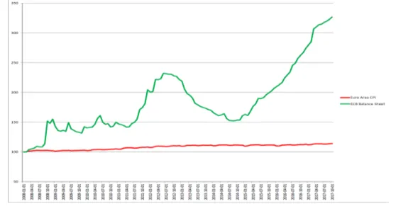
cash-Speci…cally, it presents a general equilibrium analysis of money creation by banks and of how certain policies of the central bank improve e¢ ciency over the market allocations. This analysis results in new insights on the mechanism in which the quantitative easing policy (QE) works, based on which this paper o¤ers an explanation for the observation that the QE, while causing enormous monetary expansion, is associated with low in‡a-tion or even de‡ain‡a-tion pressure in certain economies. One of them is the Euro Area, as is illustrated below:
Figure 1: The balance sheet of the European Central Bank (ECB) and the Consumer Price Index in the Euro Area over 01/01/2008-01/10/2017, with 01/01/2008 = 100. The three
hikes in the ECB’s balance sheet during the period are associated with only slight price increases, if anything at all. Source of the data: https://fred.stlouisfed.org/.
The model economy of the paper is populated by workers, entrepreneurs and banks. Workers can produce the consumption good, corn, in autarky, or work for entrepre-neurs. The specialty of banks is modeled with the assumption that workers accept
in-advance (CIA) both study monetary policy, but the former abstracts banks completely, while the latter, when concerned with money creation by banks, lets the scale of banks’ lending pinned down either by a binding reserve constraint (see e.g. Goodfriend and McCallum 2007), or by an exogenous rule of holding excessive reserves (see e.g. Chen forthcoming and Mishkin 2016), which leaves little role to banks’own decisions .
banks’promise to pay, but not entrepreneurs’, as a means of wage payment. At date 0, therefore, entrepreneurs …rst borrow banks’ promises to pay – more speci…cally, notes that read like "X bank promises to pay the bearer 10 kilogram of corn tomorrow" – and then use these notes to hire workers. As a result, entrepreneurs owe a debt to the lender banks and banks to the workers. At date 1, entrepreneurs produce corn and use it to settle their debts to the banks. Banks then use this repayment and their own corn, which is stored over time and represents their wealth, to redeem their notes from the workers by ful…lling the promises written on the notes.
In this economy, the real resources are workers’ labor and entrepreneurs’ capital, and e¢ ciency is measured with the number of workers that entrepreneurs hire. Banks matter, however, because entrepreneurs need to borrow their liabilities to hire workers. How much banks lend in terms of real value determines how many workers entrepreneurs hire and hence economic e¢ ciency. The aggregate lending of banks is in turn determined by competition between them. What banks supply is a means of payment, which is a homogenous good. They thus engage in Bertrand competition. Moreover, what a bank lends is its liability. Hence the scale of its lending is anchored to its wealth by a borrowing constraint.3 Put together, banks are engaged in Bertrand competition with a limited capacity à la Kreps and Scheinkman (1983). If the borrowing constraint is binding, banks’ aggregate wealth determines the quantity of money supplied to entrepreneurs, and hence e¢ ciency. If this wealth is below a threshold, the money supply is inadequate and so is the number of workers that entrepreneurs hire.
This problem of meagre bank wealth depressing economic activity has been diagnosed in many studies such as Holmstrom and Tirole (1997) and Gertler and Kiyotaki (2010). However, these studies are not concerned with means of payment. Hence they do not consider the possibility of a remedy with the central bank (CB) issuing …at money. By contrast, in this paper the CB can o¤er a remedy by allowing banks to borrow its …at
3This borrowing constraint could be due to a moral hazard friction à la Holmstrom and Tirole (1997)
money at zero interest up to a bound. We show that although the economy lasts for only two periods, in one equilibrium the …at money circulates, ‡owing through banks to entrepreneurs, who thereby hire more workers. That is, the policy eases the constraints imposed upon their economic activity by an inadequate supply of bank-created money. Hence, the policy is calledquantitative easing policy, or QE.
The QE enables banks to raise lending capacity without violating the borrowing constraint, while backing by the same amount of wealth. It does so because …at money is di¤erent in nature to bank-created money. A central bank never commits to redeem its …at money at a speci…ed value, whereas bank-created money is the bank’s liability, which it commits to redeem at a pre-speci…ed value and thus bears a real obligation of repayment.4 To this di¤erence in nature that Tobin (1963) alludes above. As …at money is not redeemable, its value freely adjusts with the state of the economy. In particular, its value falls in the event of the negative productivity shock, which means
in‡ation. In‡ation reduces the real value of banks’liability to the CB and thus slacks their borrowing constraint giving them room to increase lending.5
While the QE induces in‡ation in the event of the negative shock, it induces de‡ation in the event of the positive shock. This result might partly explain the aforementioned observation that in some economies the QE causes a great monetary expansion on the one hand and is companied with or followed by lingering low in‡ation or even de‡ation pressure on the other hand, which is a puzzle if considered from the point of view of
4In the model economy, this fact is straightforward because banks use corn, the real good, to redeem
their liability. Even if they redeem it with …at money, which is typically the case in the modern times, they still need to spend real resources to obtain it. Hence bank-created money still bears real obligations of repayment. For more discussion, see the remark on pages 28-9, Section 5.
5The point that monetary policy can help banks by a¤ecting the real value of their liabilities is also
considered by Diamond and Rajan (2006). Also, the way in which …at money circulates in the model economy is also in Allen and Gale (1998). However, these papers are not concerned with banks lending their liabilities to real sectors to be used as means of payment, nor with the ine¢ ciency related to banks’wealth, nor with the quantitative easing policy.
quantitative theory of money. A key di¤erence to it is that in this paper the money created with the QE is utilized to expand real economic activity resulting in a rise in the output of goods, which keeps the price down. Indeed, all the QE-created money is utilized this way if the scale of the QE is below a threshold. If it is beyond it, the excess is not put into circulation, we also …nd. This …nding partly explains another related observation, that in some economies a substantial fraction of the monetary bases created with the QE is not lent out but stays in banks’reserve accounts.
This paper is in line with nascent literature that examines banks’specialty of their liability being accepted as a means of payment. Most closely related is Donaldson, Piacentino and Thakor (forthcoming). Both their paper and this one consider how banks’ issuance of means of payment a¤ects the real economy as well as policy impli-cations. The two papers, however, have di¤erent focuses. Their paper explains how this specialty of banks is derived from their superior technology of warehousing, while this paper emphasizes the importance of banks’ wealth for economic e¢ ciency. Also the policy implications are di¤erent. Their paper shows that, contrary to the received wisdom, a higher central-bank rate could raise bank lending, while this paper considers the QE. Jakab and Kumhof (2015) describe in detail how banks create money with dou-ble book-keeping. They focus on the quantitative implications of this facet of banking in a full ‡edged dynamic stochastic framework, but are not concerned with economic e¢ ciency and policy responses, on which this paper focuses.
Since the recent crisis, many studies have examined the QE; see Gertler and Karadi (2011) and Gertler and Kiyotaki (2010), among others. Their diagnosis on the source of the problem is shared by this paper: banks’ wealth is too low causing inadequate lending.6 However, those studies model banks not as issuers of means of payment, but
as intermediaries of trading real goods. As a result, in those studies what the government issues must be backed by tax incomes and is essentially the sovereign debt, whereas what
6This is also true in a study by Brunnermeier and Sannikov (2013), where money plays the role of
the central bank issues in this paper is purely nominal. Furthermore, the mechanism in which the QE works is di¤erent. In those studies, it works by transferring wealth to banks, whereas in this paper it works by reducing the real value of banks’liability via in‡ation.
Other cases of ine¢ ciency in connection with private issuance of means of payment are considered by Hart and Zingales (2015), Monnet and Sanches (forthcoming), and Stein (2012). In Hart and Zingales (2015) and Stein (2012) ine¢ ciency is driven by …re sale externalities. In Monnet and Sanches (forthcoming) ine¢ ciency arises because banks o¤er a return rate on the liability side that is lower than the inverse of time discount. Besides this di¤erence in the source of ine¢ ciency, none of those studies considers the circumstance of banks under-lending or the policy of QE, as this paper does.
The rest of the paper is organized as follows. Section 2 sets up the model. Section 3 analyses a benchmark case where banks face no borrowing constraint, thus subject to unfettered forces of competition. This analysis not only examines the bank compe-tition in the purest form, but also bears relevance to the historical banking. Section 4 introduces the borrowing constraint of banks. Section 5 studies the QE and Section 6 interest rate policy and capital-adequacy regulation. Section 7 concludes. All proofs are relegated to Appendix.
2
The Model
The economy has one storable good, corn, used as the numeraire, and lasts for two days. Contracting and production occur at t = 0; yielding and consumption at t = 1. There are N banks, N2 entrepreneurs and N3 workers, where N is a large number (later, in
section 5, the central bank will be introduced).7 Thus, banks are in perfect competition
7A setting with the same feature is to be found in Wang (2015), where continuum of [0;1] and
and each serves a large number of entrepreneurs; and there are more workers than entrepreneurs can hire. All agents are risk-neutral and protected by limited liability.
Workers either produce w kilograms (kg) of corn in autarky, or are hired by entre-preneurs, who each have h units of human or physical capital. If an entrepreneur hires
L workers att= 0;then his project yields at t= 1
y=Ahe 1 L ;
where 0 < < 1: Without losing any generality, normalize h = 1: Productivity, A;e is subject to a common shock. At t = 0; it is common knowledge that the good state with Ae = A occurs with probability q > 0 and the bad state with Ae= A occurs with probability1 q >0. Let Ae qA+ (1 q)A denote the mean. Assume:
0< A < Ae : (1)
As there are more workers than can be hired by entrepreneurs, in equilibrium workers are indi¤erent in working for the latter or in autarky. Therefore they earn a real wage of w. This wage is independent of economic activity of the other sectors, which gives a convenience for exposition.
Banks each haveG units of corn, where a unit is de…ned asN kg and used wherever banks are concerned. Banks supply no real resources for corn production. What makes banks relevant is due to the following assumption.
Assumption 1: Workers do not accept entrepreneurs’ promise to pay but banks’ as a means of wage payment.
This assumption captures the specialty of banks explicated in the Introduction. Ac-cording to Kiyotaki and Moore (2001), this di¤erence between banks and entrepreneurs arises because the former has stronger commitment power than the latter.
Due to this assumption, entrepreneurs cannot hire workers att= 0with a promise to pay them later at t= 1:To hire workers, enterpreneurs need to borrow banks’promise to pay them at t = 1. We assume that banks have no di¢ culty enforcing repayment
from entrepreneurs and hence this borrowing is feasible. To …x the idea, suppose that banks’ promises to pay are printed on notes. That is, a note issued by a bank reads that this bank promises to pay the bearer of this note with a certain quantity of corn att = 1:8 This quantity is the note’s face value or par value.
Assumption 2: The face values of banks’notes cannot be contingent on the real-ization ofA:e
This assumption captures the observation that in real life a private security that serves as a means of payment, such as demand deposit, promissory notes, cheques, or trade credit, commonly bears …xed claims and is of debt, and is rarely a contingent claim.9
Besides the friction of payment, entrepreneurs lack commitment power in another dimension.
Assumption 3: entrepreneurs are unable to make commitment on the scale of their projects in terms of the number of workers they will hire.
This friction is real in the sense that it is unrelated to means of payment. In the absence of the friction, a bank would be willing to lower the interest rate, denoted by r; to a borrower entrepreneur who commits to a smaller scale, because thereby his project delivers a higher average return rate. This, however, would give entrepreneurs an incentive to borrow from multiples banks, each in a small amount and thus at a favorable rate. The presence of the real friction, therefore, is justi…ed if entrepreneurs cannot be prevented from doing so. The importance of its presence is that it engenders a wedge between the …rst- and second-best allocations, as will be shown.
8In the model economy banks promise to pay the real good in redeeming their liability, whereas
in modern times, they typically redeem it with …at money, the central bank’s issues. Other instances of claims on real goods used as a means of payment incude Hart and Zingales (2015) and Williamson (1999). This abstraction is harmless in the baseline model where in‡ation is not concerned with. Where it is, as in Section 5 below, the abstraction helps clarify the mechanism in which the QE works.
9For why that is the case, see Gorton and Pennacchi (1990) and Dang, Gorton and Holmstrom
Due to the friction, a bank posts a single interest raterfor loans of any sizeE rather than a menu ofr(E). A loan contract is represented by a pro…le of(E; r): att = 0, the entrepreneur borrows the bank’s notes of overall face valueE and att = 1 he is obliged to payE(1 +r) kg corn back to the bank.
The timing of events is as follows.
Att= 0;each bank posts the aggregate face value of notes that it will issue,D;and the interest rate that it will charge,r: Observing all these o¤ers, each entrepreneur then chooses one bank to go to and asks to borrow faceE of the bank’s notes. If one bank’s notes are over-demanded, only a fraction of the entrepreneurs have their demand met. Entrepreneurs then use borrowed notes to hire workers and start the production. Banks store their Gunits of corn.
At t = 1; entrepreneurs produce corn. They either repay E(1 +r) kg corn to the lender banks or default. In that case they give all their output of corn to the banks. After receiving repayments from the entrepreneurs, the sum total denoted byY ;e banks redeem notes from workers. If Ye +G D to a bank, its notes are redeemed at par. If
e
Y +G < D; the bank defaults and the notes are redeemed at fraction Ye +G =D of their par values. Finally, the agents consume the corn in their possession.
In anticipation of the possibility of default, at t = 0 a bank’s notes are discounted with factor of
=EAe[min(1;Ye +G
D )]: (2)
Passing on to the equilibrium analysis, we …gure out two benchmark allocations.
The First-Best and Second-Best Allocations
E¢ ciency concerns the number of workers allocated to entrepreneurs. De…ne the …rst-best allocation as the number of workers that maximizes the social surplus of projects, which is AeL wL due to universal risk neutrality and the opportunity cost of labor being w:The …rst-best allocation is thus
LF B = (Ae
w )
1 1 :
The second-best allocation is de…ned as the number of workers that entrepreneurs would hire in the competitive equilibrium if the friction of payment (in Assumption 1) were absent, but the real friction (in Assumption 3) remained. That is, if entrepreneurs could hire workers with their own promise to pay, but their wage o¤er could not be conditional on the scale of their projects. The equilibrium allocation is as follows.
Lemma 1 The second-best number of workers that entrepreneurs hire is:
LSB = (qA + (1 q)A
w )
1 1 :
Obviously, LSB > LF B. That is, the real friction induces the entrepreneurs to hire too many workers.10 This fact engenders a circumstance of banks over-lending, among
remedies to which are interest rate policy and capital adequacy regulation, as will be shown in sections 4 and 6.
Below we …rst analyze the baseline model in which bank issuance is subject to no borrowing constraints, nor any other restrictions. This analysis serves two purposes. One, it studies the competitive equilibrium of money creation by banks in the purest form. The other, the analysis bears relevance to early periods of the banking history.
3
The Least Fettered Issuance
In the least fettered issuance, banks can …nance an unlimited quantity of assets by issuing promises to pay. The equilibrium quantity is of course limited, as examined below. We …rst consider the demand side of the market for banks’ notes, then the supply side, and, …nally, the meeting of the two.
3.1
The Demand Side of the Market for Notes
Consider a representative entrepreneur who borrows from a bank o¤ering (D; r): If he borrows notes of a face valueE, then they are worth E;where the discount factor ;as will be shown, is a function of(D; r). With these notes, he hires workers in a number of
L= E
w ; (3)
because they earn real wagew:Att= 1;the entrepreneur either repaysE(1 +r)of corn to the bank or defaults. Thus, his decision problem is:
max
E EAe[max(ALe E(1 +r);0)]; s:t:(3):
Lemma 2 For any(w; ; r), the solution to the above problem satis…esAL < E(1 +r). That is, entrepreneurs all default in the bad state.
This lemma is driven by the assumption thatA < Ae ;which says that the negative shock is severe enough to knock entrepreneurs into default.
At the optimum, the demand of the representative entrepreneur for the notes is
E( ; r) = ( A 1 +r) 1 1 ( w) 1 (4)
and the number of workers that he hires and his pro…t are, respectively,
L(R) = (A wR) 1 1 (5) V(R) = q(1 )(A 1 wR ) 1 ; (6) where R 1 +r: (7)
Note that so de…ned R is the actual interest rate and measures the cost of borrowing: To obtain a means of payment that is worth 1, the entrepreneur borrows notes of face
value1= ; then in a debt of(1 +r)= : Naturally, his scale of hiring and his pro…t, which are both real variables, are inversely related to the cost of borrowing, namely,R:
Recall that the e¢ ciency concerns only the number of the workers hired by entre-preneurs, which depends only on the actual interest rate. The e¢ ciency of market equilibrium is thus determined solely by the actual interest rate in equilibrium. De-…ne RF B (RSB)be the value of the actual interest rate at which entrepreneurs hire the …rst-best (second-best) number of workers, that is, L(R) = LF B (LSB): With (5),
RF B = A
Ae
RSB = A
qA + (1 q)A:
After banks all have posted (D; r), each entrepreneur decides which bank to go to. In the equilibria of this subgame, an entrepreneur gets the same expected pro…t,Vb, from any bank who attracts a number of entrepreneurs.11 As entrepreneurs’pro…t depends only on the actual interest rate, de…ne Rb by V(Rb) = V :b Then, Rb is the actual interest rate that prevails on the notes market, conditional on banks’ choices of (D; r): Given that there is a large number of banks, any single bank is too small to a¤ect Rb with its choice of (D; r) and takes it as given when making that choice.
3.2
The Supply Side of the Market for Notes
Consider a representative bank. To attract entrepreneurs to come, the bank’choice of
(D; r) satis…es V(R) Vb or, equivalently, (1 +r)= R:b While the interest rate r is directly chosen by the bank, the discount factor of its notes is determined by (D; r). It depends on whether the bank ever defaults or not, that is, whether D > Ye +G in
11By o¤ering(D; r);which determines ;each bank chooses an actual interest rateR= (1 +r)= :No
entrepreneur goes to a bank o¤eringV(R)<Vb when he can getVb elsewhere. On the other hand, if a bank o¤ersV(R)>Vb, it induces over-demand for its notes (which is never optimal), so an entrepreneur coming to it is served with such a probabilityl thatl V(R) =Vb.
some state att = 1:In the good state, Ye =Y =D(1 +r)because the entrepreneurs do not default. As a result, the bank does not default. In the bad state, by Lemma 2, all the entrepreneurs default and pass the output of their projects on to the bank, of which the aggregate value is given below:
Lemma 3 The aggregate value of the bank’s loans in the bad state is
Y = A
A D(1 +r):
12 (8)
In the bad state, the bank does not default if and only ifD G+Y ;which, with Y
given by (8), is equivalent to
D (1 A(1 +r)
A ) G: (9)
On the left hand side is the loss made by lending in the bad state, D Y : Thus, the inequality says that banks will stay solvent in the bad state if and only if their lending scale, D, is not too large relative to their wealth, G, so that the loss from loans can be absorbed by the wealth.
Substitute the value of Ye given above into (2), and the discount factor of the bank’s notes is determined by its choice of(D; r) via:
(D; r) = 8 < : 1, if (9) is satis…ed q 1 + (1 q) (G D + A(1+r) A ), otherwise 9 = ;: (10)
Now consider the representative bank’s decision problem at t = 0: Taking into ac-count the possibility of default, its economic pro…t with the choice of(D; r), denoted by
(D; r), isEYemax(G+Ye D;0) G: Lemma 4 (D; r) = D 1 +r RSB : (11) 12Y < Y becauseA < A e by assumption andAe < A :
Therefore, the pro…t margin of lending, that is, the pro…t of lending out a note of face value 1, is(1 +r)=RSB :Intuitively, the present value of this note, which is part of the bank’s liability, is ; while the bank’s revenue from such lending is EYe Y =De = (1 +r)=RSB:
The representative bank chooses(D; r)to maximize (D; r)subject to the constraint that it can attract entrepreneurs to come, that is,
1 +r
(D; r) R:b (12)
Given the scale of lendingD, the bank wants to charge an interest rate as high as possible so long as it can attract entrepreneurs. Therefore, at the optimum, the constraint (12) is binding.13 Hence, the bank’s optimal choice of r as a function of its choice of D;
denoted byr(D);is determined by
1 +r
(D; r) =R;b
and banks’problem becomes
max D D (D; r(D)) " b R RSB 1 # :
As > q always (because the bank always redeems its notes at par in the good state), the following proposition is self-evident.
Proposition 1 The solution to and the value of the representative bank’s problem are: (i) if R > Rb SB; then D=
1 and =1;
(ii) if Rb = RSB; then = 0; and the bank is indi¤erent to any value of D, with
r=r(D);
(iii) if R < Rb SB; then lending makes a loss, and thus D= 0 and = 0:
As was shown, the pro…t margin of lending equals R=Rb SB 1 and is positive if and only ifR > Rb SB: Moreover, if the pro…t margin of lending is positive, banks obtain
13Mathematically, givenD;both 1+r
SB (D; r)and
1+r
=1: That is because, despite their limited stocks of corn, they all have an unlimited lending capacity (i.e. D =1); due to two reasons. One, what banks lend out is their promise to pay, essentially word of mouth, which they can in…nitely supply. The other, banks are subject to no constraints on the quantity of supply in the baseline model.
3.3
The Equilibrium: The Second-Best Allocation Attained
The prevailing actual interest rate, R;b which plays the role of price, clears the market for notes in equilibrium. We de…ne the symmetric equilibrium below and discuss other equilibria later.
De…nition 1 A pro…le (fD; r; ; Eg;Rb) forms an equilibrium if:
(i) given R;b banks’choice of (D; r) is optimal and thus given in Proposition 1. This choice determines = (D; r) through (10);
(ii) given that all banks o¤er the same (D; r; ); entrepreneurs go to each bank with the same probability and by the Law of Large Numbers, each bank receive N of them. Their demand for notes, E; is optimal, that is, E =E( ; r) given by (4);
(iii) the market clears: D=E:14
In any equilibrium, banks neither obtain an in…nitely large pro…t, nor abstain from lending, which, by Proposition 1, is the case if and only if
b
R =RSB:
Therefore, the real allocation in equilibrium is unique and conforms with the second-best allocation, the one that would arise if the friction of payment were absent and entrepreneurs could hire workers with their own promises to pay. Intuitively, what banks supply is a mean of payment, a homogeneous good. Furthermore, in this case of unfettered issuance, they all have unlimited capacity. Therefore, they are in Bertrand
competition, which annihilates their pro…t margin. As a result, entrepreneurs overcome the friction of payment at no costs and the real allocation is the one that would arise if the friction were absent, that is the second best allocation.
On the nominal side, however, there is indeterminacy. AtRb=RSB;by Proposition 1, the pro…t margin of lending is 0, and individual banks are indi¤erent to any quantity of issues, although in aggregation, their issues exactly su¢ ce for entrepreneurs to hireLSB workers. This indeterminacy leads to a continuum of equilibria besides the symmetric one de…ned above. In the symmetric equilibrium, all banks issue the same quantity of notes and their notes are discounted at the same factor, therefore, one bank’s notes are perfect substitutes for another’s. In asymmetric equilibria, however, some banks issue more than others despite ex ante being identical, and see their notes more heavily discounted.
Proposition 2 (i) In any equilibrium, independent of banks’ wealth G, Rb =RSB; the pro…t margin of bank lending is 0, and the second-best allocation is attained.
(ii) In any equilibrium, a fraction of banks default at t = 1 upon the realization of
e
A=A if and only if banks’wealth is below a threshold G ; where
G = [(qA + (1 q)A) A](qA + (1 q)A
w )
1 :
An intuition for result (i) is given above. As for (ii), note that given banks are indi¤erent to any quantity of issues, the quantity of money circulated, that is, the aggregate bank lending, is determined by the demand side, namely entrepreneurs. Thus, the aggregate bank issues are …xed at a quantity exactly su¢ cient for entrepreneurs to hire the second-best number of workers. With this scale of lending, if banks’wealth,G, is su¢ ciently low –namely G < G –then it is insu¢ cient to absorb the loss incurred in the bad state and bank default occurs accordingly.
The baseline mode examined above, besides providing a simple framework to consider money creation by banks on competitive markets, also bears empirical relevance to the
early periods of the banking history during which a large number of banks issue their own notes and discount others’, such as the Free Banking Era in the U.S. (1838-1863) and a period between 1750-1844 in England.15 Speci…cally, the baseline model derives relationship between the loan interest rate r, the discount factor , the leverage ratio
:=D=G;and the risks of default1 qof individual banks. First, 1+r =R;b a constant across banks, by the binding constraint (12). Therefore, the paper predicts that across banks, the gross interest rate that a bank charges for loans (i.e. 1+r)is positively related to and solely determined by the discount factor of its notes , independent of the bank’s other attributes. Second, regarding the discount factor, from (10) and binding (12) it follows that = 8 < : 1 if (1 A A Rb) 1 q+(1 q) 1 1 (1 q)A A Rb if (1 A A Rb) 1 9 = ;: (13)
Therefore,the discount factor of a bank’s notes is inversely related to the bank’s default risk 1 q16 and its leverage (which is endogenous). The …rst part of this prediction
is empirically con…rmed by Gorton (1999) who studies the pricing of banknotes during the U.S. Free Banking Era.17
The applicability of the baseline model to the modern banking is more limited. A fundamental assumption of the model, namely that banks face no constraints in making loans, is probably far from reality nowadays. In particular, due to this assumption, the
15For the case of the U.S., according to Gorton (1999), thousands of di¤erent banks’ notes were in
circulation, while for the case of the England, Cameron et. al. (1967) report that in year 1810 there were 783 note issuing county banks in England.
16In the lower branch of (13)@ =@q share the sign of 1 A A Rb
1; which is positive because in
that branch (1 A
A Rb)
1;that is, 1 1 A A R:b
17Speci…cally, he found that possessing traits of low default risks, such as being a member of the
Su¤olk System or under a state sponsored insurance, is negatively correlated with theimplied volatility
of the bank, of which the discount factor –or price in his paper –is a decreasing function. Therefore, the low-risk traits are associated with a higher value of .
baseline model predicts that the aggregate quantity of bank credit is independent of banks’wealth,G;whereas the aftermath of the recent …nancial crisis witnesses that the banking sector reduces credit issuance after su¤ering a severe loss. To give an account for this observation in particular and to examine the modern banking in general, we shall introduce a borrowing constraint to banks, as below.
4
Banks’Wealth Matters in the Presence of a
Bor-rowing Constraint
In this section, we assume banks are subject to a borrowing constraint, that their equity value should never fall below (1 )G:18 The equity value is higher in the good state
than it is in the bad state. Thus, we only need to consider the constraint in the bad state, which is G+Y D (1 )G: With Y = A(1 +r)=(A ) D by (8) and rearrangement, it becomes:
D 1 A(1 +r)
A G: (14)
The introduction of the constraint has two immediate implications. One, as banks always maintain a positive equity value, they never default. Therefore, their notes are not discounted, that is, = 1 and hence1 +r =Rbhereafter. As a result, the borrowing constraint (14) becomes
D 1 A
A Rb G: (15)
18This borrowing constraint can be due to several reasons. One, in the modern times bank default
becomes very costly and banks’ managers want to maintain solvency in any contingency, which is a special case of the above constraint with = 1: Another, as is in Holmstrom and Tirole (1997) and Getler and Kiyotaki (2010), banks have a moral hazard issue: at t = 1; the owner of a bank – the banker – can abscond with a fraction of1 of its stored wealth to a remote island. Hence, banks’ equity value should never fall below(1 )Gin any contingency.
The other, unlike in the preceding case of least fettered issuance, banks now are in Bertrand competition withlimited capacities à la Kreps and Scheinkman (1983). With the borrowing constraint, the market equilibrium is as follows.
Proposition 3 (i) If G 1G ; then in all equilibria the real allocation is the same as in the case of least fettered issuance: Rb = RSB; the pro…t margin of bank lending is 0,
and L=LSB:
If G < 1G ; there is a unique equilibrium in which the pro…t margin of bank lending is positive; and R > Rb SB and Rb is determined by G through
G= 1(A w ) 1 1 1 A A Rb b R11 G(Rb): (16)
(ii) If G decreases from 1G to 0 the equilibrium interest rate, R;b increases from
RSB to A =A and the number of workers hired by entrepreneurs decreases from LSB to
LSB [ A
qA +(1 q)A]
1 1 :
The borrowing constraint limits banks’capacity of issuance to an endogenous pro-portion of their wealth. If their wealth is high enough – that is, beyond 1G – then
banks still possess a capacity large enough to annihilate the pro…t margin of issuance, which leads to the second-best allocation, as was in the case of least fettered issuance. Hence arises result (i).
If G < 1G ; banks’ wealth does not su¢ ce to back an issuance of that size. As a
result, issuance bears a positive pro…t margin. This positive pro…t margin drives all banks to issue as much as possible, until the borrowing constraint, (15), is binding. This clears the indeterminacy in the quantity of individual banks’issues and gives rise to a unique equilibrium. It also shows that, now, the quantity of money circulated is determined by the supply side – namely, the banking sector – rather than by the demand side, as was in the case of least fettered issuance. Therefore, the lower the banks’wealth, the lower the total value of money that they supply and, as a result, the
higher the interest rate of borrowing (Rb) and the fewer the workers that entrepreneurs hire.
The last comparative static, however, does not mean the aggregate output always decreases withG forG < 1G because of the wedge between the …rst-best and second-best allocations, namely LF B < LSB. De…ne
GF B G(RF B);
where functionG(Rb) is de…ned in equation (16); withRF B =A=Ae,
GF B = 1(Ae A)(Ae =w)1 :
Then GF B is the level of banks’wealth at which the actual interest rate exactly takes the …rst-best value and therefore the aggregate output is maximized. GF B < 1G .19 By
Proposition 3, then, there are two types of e¢ ciency.
(1)G < GF B:In this case, R > Rb F B andL < LF B: That is, relative to the …rst-best allocation, banks under-lend, whereby the cost of bank credit is too high and the sector that depends on it –namely entrepreneurs –obtains inadequate resources, namely labor. (2)G > GF B:In this case, R < Rb F B andL > LF B: That is, relative to the …rst-best allocation, banks over-lend, whereby the cost of bank credit is too low and the sector that depends on it obtains excessive resources.
The existence of the second type of ine¢ ciency is due to Assumption 3, which drives a wedge between the …rst-best and second-best allocations. In the absence of this wedge,
RF B would be equal to RSB; hence G(RF B) to 1G ; and the case of bank over-lending
would not exist. This case of over-lending provides the paper with room to accommodate interest-rate policy and capital adequacy regulation, as will be shown in Section 6.
The …rst type of ine¢ ciency is caused by inadequate creation of money by banks. Can the central bank enlarge the money supply through the banking system? It can, we show in the next section, with a policy which, as it eases the constraints imposed by dearth of money, is called the Quantitative Easing Policy, or QE.
5
The QE Slacks the Borrowing Constraint of Banks
The central bank (CB hereafter) in this economy is modeled as the unique entity that is able to costlessly produce another means of payment which has no intrinsic values; to …x the idea, let it be shells. Shells are di¤erent in nature to bank notes. The CB does not promise to pay a holder of shells with any corn, the real good. Shells, therefore, are purely nominal. By contrast, a bank commits to redeem its notes with the promised amounts of corn. Hence banks’notes are not nominal.
Although shells are …at money and the model economy lasts for only two dates, shells can circulate in it, whereby the CB can conduct meaningful monetary policy, such as the following QE. At t = 0 the CB announces a facility whereby each of the N banks can borrow up to S units of shells (again 1 unit de…ned as N kg) at a small interest rate >0:A borrower bank is obliged to repay its debt to the CB at t= 1 either with shells or with corn, with a …xed rate of exchanging corn for shells, for example, 1kg corn for 1kg shells. This exchange rate is arbitrary and is made to confer a nominal value on shells, as in real life Bank of England can print an arbitrary number, like £ 10, on a piece of paper, and then this piece of paper has a nominal value of £ 10 and can be used to buy real goods of this value (e.g. two packs of cherries at M&S). As such, we call 1kg corn as thepar value of 1kg shells etc., although shells are nominal. The banks that have used the CB’s facility thus have two types of money to lend to entrepreneurs. One is their own notes, the other shells. We assume that no entrepreneurs borrow both types of money in order to avoid the unnecessary complication of which debt of the two is senior in case of default.
The contract of borrowing a bank’s notes is still represented by (E; r), whereby the entrepreneur borrows the bank’notes of face value E at t = 0 and then owes it a debt of E(1 +r), which he repays at t= 1 with corn.
The contract of borrowing shells is similarly represented by (Es; rs) whereby the entrepreneur borrowsEs kg shells att= 0 and then owes the bank a debt ofEs(1 +rs),
which he repays at t = 1 with either corn or shells, with 1kg corn equivalent to 1kg shells.
The timing of events at t = 0 is as follows. First, the CB chooses S and publicly announces the policy. Then, banks decide the quantity of shells to borrow from the CB,
Q S;and post o¤ers of(D; r;Q; rs):Based on these o¤ers, entrepreneurs decide which bank to go to and how much they borrow. Lastly, they use borrowed means of payment (bank notes or shells) to hire workers and start the production.
The timing of events at t = 1 is as follows. First, entrepreneurs produce corn. Second, the market for shells opens, on which the shell-borrowing entrepreneurs use corn to buy shells from workers. Let p1 (p1) denote the shell price in the good (bad)
state. Third, entrepreneurs settle their debts to the lender banks, using corn and/or shells. Fourth, the market for shellsmay open the second time, on which banks having excessive shells sell to banks in shortage. Lastly, banks redeem their notes from workers and settle their debts to the CB. At this stage, the CB may end up with holding a certain quantity of corn, which it will transfer to the agents of the economy before the consumption starts.
Note that there is no surprise or nominal rigidity associated with the QE. All the private sector agents (i.e. banks, entrepreneurs and workers) made decisions after having observed the CB’s move and they can freely adjust their decisions with it. Still, the QE produces real e¤ects in this economy in one equilibrium ifG < 1G .20 For anyG < GF B; moreover, there exists a unique value ofS at which this equilibrium attains the …rst best allocation. This is the equilibrium that we discuss below.
20As shells are …at money, there is another equilibrium in which workers disbelieve that shells will
have real value at t = 1 and thus do not accept to be paid with shells att = 0; which are thus not circulated. This type of equilibria exists for …at money in general. By contrast, they never exist for banks’notes: banks each have Gunits of corn, therefore their notes always have a positive real value att = 1; indeed, if a bank issuesD G;workers know, without any equilibrium calculation, that its notes are worth at par. This di¤erence results from the di¤erence in nature between shells and banks’ notes stated at the beginning of this section.
In this equilibrium, at t = 0, workers believe that they will be able to use shells to buy corn at t = 1 and thus they accept a wage payment with shells; and at t = 1, indeed shells receive a positive real value, intuitively because they can be used to settle certain debts that otherwise have to be settled with corn. To solve the equilibrium, we …rst examine what happens at t = 1 and then that at t = 0: Consider, …rst, the case in which S is below a threshold (which is given in Proposition 4 below) and therefore
rs> in equilibrium. In this case, all the banks borrow to the full capacity of the QE, namely,Q=S;and lend all the shells out to entrepreneurs. Therefore, at the beginning of t = 1; there are N S units of shells in workers’hands and the aggregate debt of the shell-borrowing entrepreneurs isN S (1 +rs)units.
In the good state, as no entrepreneurs default, the shell price p1 = 1. On the one
hand, shells can never be worth more than their nominal values: if the entrepreneurs use 1kg corn only to buy less than 1kg shells, they will not buy them, but use 1kg corn to settle a debt of 1kg shells to the banks. On the other hand, in the good state, it cannot be that p1 <1 either. Otherwise, the shell-borrowing entrepreneurs would want
only shells, not corn, to repay all their debts. Their aggregate demand for shells would thus be N S(1 +rs); as they do not default. This demand, with rs > 0; is bigger than
N S;the supply of shells, leaving the market uncleared.
As p1 = 1, the entrepreneurs are indi¤erent to repaying their banks with shells or
with corn in the good state. As a result, some banks may end up with more thanS(1+ )
units of shells, some less. If so, the former wants to sell the excess to the latter and the second shell market opens. On this market, the equilibrium shell price,pB;equals 1 also, following the same argument as above. On the one hand, it impossible thatpB >1: On the other hand, if pB <1;banks all want to use only shells, not corn, to settle their debts to the CB, and their aggregate demand would beN S(1 + );greater than the total supply,N S;thus the market uncleared. This argument holds true, and hence pB = 1 is the only market clearing price, so long as >0;however small. To simplify exposition,
in what follows, we consider the limit case where !0.21
In the bad state, the output is low. Hencep1 <1;as will be veri…ed later. Thus, the
shell borrowing entrepreneurs use only shells, no corn, to repay the banks. Furthermore, in this state entrepreneurs all default according to Lemma 2. This means all their outputs are used to settle their debts to the banks. These two facts put together, all the shell-borrowing entrepreneurs’output is used to buy shells. Denote byYs the total output of one bank’s shell-borrowing entrepreneurs. Then the shell market clearing commands that p1 N S=N Ys;or
p1 =Ys=S: (17)
With a calculation similar to that leading to equation (8), we …ndp1 =A(1 +rs)=(A ); which, as is shown below in Proposition 4, is smaller than 1 indeed, as was intuitively argued. Moreover, from p1 = Ys=S it follows that the shell-borrowing entrepreneurs of one bank altogether buy Ys=p1 = S units of shells. Hence, each bank ends up with
having S units of shell equally and the second shell market does not open in the bad state.
The value of 1 kg shells at t= 0; p0; is the mean of their values att= 1:
p0 =q 1 + (1 q)
A(1 +rs)
A : (18)
Workers thus accept a wage payment withw=p0 kg shells att= 0 in the equilibrium.
The e¤ect of this policy is presented in the following proposition:
Proposition 4 SupposeG < 1G . (i) If the QE’s scaleS < S(G) A q(A A)(
1G G),
then there is a unique equilibrium in which all theS units of shells are in circulation. In
21Note, however, that if = 0; then there is indeterminancy: any price p
B 2 [0;1] can clear this
second shell market. If = 0; the aggregate excess exactly equals the aggregate shortage. Then, the supply side is willing to sell all the excessive shells at anypB 0, while the demand side is willing to
this equilibrium, the QE produces real e¤ects: the actual interest rate, R;b is determined by S through S = ( A w ) 1 1 1 (1 q) q 1 1 1 G 1 F( ;G);with A A R:b (19)
Moreover, the interest rate of lending shells is rs = [qA +(1 q)A] b R A
A (1 q)AbR : It satis…es rs >0
and A(1 +rs)=(A )<1; as was said.
(ii) If S increases, Rb and rs decrease and L increases. At S = S(G); Rb = RSB;
rs= 0 and L=LSB:
The QE works by increasing the real value of money that banks lend out at t = 0:
That explains why, compared to the situation of its absence (namely with S = 0); the cost of borrowing money(Rb)is reduced, whereby entrepreneurs hire more workers. And the larger the scale of the QE (i.e. S), the greater are these e¤ects (so long asS is below
S(G)).
The question is: how is the QE able to make banks enlarge lending scale, backing by the same amount of wealth without breaking the borrowing constraint? To answer this question, consider a representative bank’s balance sheet att = 1; as follows:
Assets Liabilities
Corn stored (G) Equity
Loans in notes(Y) Liability to the note holders (D)
Loans in shells (Ys) Liability to the CB(p1S)
Table 1: The balance sheet (in real value) of the representative bank with the QE
Consider the bad state, in which the borrowing constraint is binding. The constraint commands that G+Y +Ys D p1S (1 )G: This inequality, with p1 = Ys=S by (17), is equivalent to G+Y D (1 )G; which leads to inequality (14), the same borrowing constraint in the absence of the QE. Therefore, the injection of the …at money with the QE does not reduce the capacity of private issuance at all. This is due to
p1 =Ys=S < p022; which means that in the bad state the shell price goes down, so that
the real value of a bank’s liability to the CB,p1S;falls enough to be covered by the value
of the assets,Ys:The decrease in the real value of shells means in‡ation. Put di¤erently, the QE enables banks to lend more without breaking the borrowing constraint because it induces in‡ation in the bad state, which lowers the real value of banks’ liability to the CB. The in‡ation arises because shells are …at money. The CB never commits to redeem shells with a real good. Their value, therefore, freely adjusts with the state of the economy. By contrast, banks commit to redeem their notes (i.e. their promise to pay) at a pre-speci…ed, noncontingent, value.23 This di¤erence in nature between banks’ notes and shells, therefore, drives the functioning of the QE.
Remark: An abstraction of the model helps elucidate this mechanism of the QE. That is the denomination of banks’liabilities with corn, the real good. In reality, how-ever, typically they are denominated with the …at money currency of the economy. Incorporating this feature would not necessarily invalidate the working of the mecha-nism. First, the aforementioned di¤erence in nature between bank created money and currency is still there. Although banks now use the currency to redeem their liability, to obtain the currency, they need to expend real resources. Therefore, their liability still bears real obligations of repayment. In contrast, …at money is not redeemable and bears no such obligations. Second, it is true that if banks’liability is denominated with the currency, its real value falls under the negative shocks, which improves banks’con-ditions. However, credit crunch still happens. So long as they face a binding borrowing
22p
1< p0,p1< q 1 + (1 q) p1,p1<1;which holds true by the proposition.
23In the model economy, the value of these issues att= 1could be made contingent on the state in
two ways. One is to let the speci…ed value contingent on the state, which is disallowed by Assumption 2. The other is default, which is disallowed because of the borrowing constraint, (14). While default is disallowed altogether because of the particular form that the constraint takes, in general so long as any borrowing constraint restricts banks’capacity, there is only a limited extent to which the value of their liabilities can adjust to the real economic conditions.
constraint, they will still reduce lending if their wealth is profusely eaten o¤, as is ev-ident in the aftermath of the 2008-9 crisis. Third, in this circumstance, if the QE is able to raise banks’lending capacities, it has to slacken their borrowing constraint. As it does not give real resources to banks, to do so it has to further reduce the real value of banks’ liability and this can only be done via in‡ation. Fourth, this reduction can be done by the CB with the QE, but not by banks themselves, exactly because of the above said di¤erence in nature between the two types of money.
At core is the point that this di¤erence gives the CB a leeway to act that banks do not have. This point can be seen even more clearly in a modi…ed version of the setting where the CB implements the QE by directly lending shells to entrepreneurs (rather than through banks) at interest rate rs, which would result in the same prices of shell and the same allocation as in the original setting. Obviously in this setting the CB can lend out the currency, whereas banks cannot lend more of their liabilities, because shells are not redeemable but banks’ liabilities are. Moreover, if banks’ liabilities were now denominated with the currency, this policy would still work. Actually it would work better because it would slack banks’borrowing constraint by inducing in‡ation, which enables them to enlarge the lending capacity.
Back to the model, while the QE induces in‡ation in the bad state, it causes de‡ation in the good state: p1 = 1> p0: This result might partly explain the lingering de‡ation
pressure or the low in‡ation observed during or after the implementation of the QE in several economies, such as the U.K. and the Euro zone. This phenomenon would be a puzzle if considered from the point of view of the quantitative theory of money, given that the QE enormously expands the monetary base.
Thus far we have considered the case in whichS < S(G) and therefore rs>0:Now we consider what happens if the QE is in a bigger scale. At S =S(G); Rb = RSB and
rs= 0: By Proposition 1 (iii), Rb can never fall below RSB, otherwise banks would stop lending altogether, not a case in equilibrium. Therefore, if the scale of the QE is larger
than S(G); then Rb stays atRSB; rs at 0, and the excessive shells beyond the threshold are not put into circulation; indeed, withrs = 0;banks are indi¤erent with any quantity of shells to borrow and lend. This result partly o¤ers an explanation for the phenomenon that in certain economies such as the U.S. and the Euro Zone, a substantial fraction of monetary bases created with the QE is not lent out but stays in banks’reserve accounts. Now consider the optimal scale of the QE. The …rst best value of the interest rate is Rb = RF B. In the circumstance where G GF B and hence Rb RF B at S = 0, anyS >0 only makes Rb still smaller and e¢ ciency even lower. Therefore, the optimal
S = 0, namely, the CB should not implement the QE at all in the circumstance of banks over-lending. However, in the the circumstance where G < GF B and hence R > Rb F B at S = 0; there is a unique value of S at which the QE drags down Rb to RF B: This is summarized below.
Proposition 5 (i) If G GF B; the optimal scale of the QE is S = 0; that is, no QE
should be implemented.
(ii) If G < GF B; the optimal S =F(A
A R
F B;G)>0, where function F( ) is given
by (19). At this scale the QE attains the …rst-best allocation (i.e. Rb=RF B):Moreover, with the optimal QE, banks earn pro…t from lending shells (i.e. rs>0);but their overall
pro…t is reduced compared to the case without the QE if G G for some G < GF B:
According to the last result, although with the QE, banks receive free funding from the CB and lend it at a positive interest rate, surprisingly they lose from the policy, which thus does not subsidize them. That is because to banks, besides this positive e¤ect on the scale, the QE induces a negative, general equilibrium e¤ect on the pro…t margin by enlarging the lending capacities of all banks. As a result, banks obtain a reduced pro…t from lending their notes. As @F=@G < 0; if banks’ wealth is above a threshold (i.e. G); then the scale of the optimal QE is small enough. As a result, the positive e¤ect from the enlargement of lending scale is small and dominated by the
negative e¤ect from the reduction of pro…t margin. However, even in this case of banks all losing from the free funding of the CB, given rs > 0, still individual banks strictly prefer taking it rather than abstaining from it – thus the QE can be conducted on a voluntary base. The reason is that a single bank takes the pro…t margin of lending as given and neglects the e¤ect on it of enlarging its own capacity.
In the circumstance whereG > GF B and banks over-lend, we have seen that the QE does not help. What the CB can do is discussed in the next section.
6
Interest Rate Policy and Capital Adequacy
Reg-ulation to Curb Bank Lending
IfG > GF B;then banks over-lend, making the actual interest rate too low and entrepre-neurs hire too many workers relative to the …rst-best allocation. In this circumstance, it is usually expected that the CB can help by setting a high policy interest rate. This idea is explored in this section, where we show that interest-rate policy produces real e¤ects and is able to attain the …rst-best allocation if and only if there is a nominal rigidity. In its absence, we show, capital adequacy regulation is always a remedy.
To explain the meaning of nominal rigidity in this paper, we de…ne nominal wage as the total face value of banks’ notes that workers receive as the wage payment. In the absence of any intervention from the CB, the nominal wage is w because banks do not default (due to the borrowing constraint 14). The nominal rigidity in this paper is de…ned as the friction that keeps the nominal wage of workers staying at w and unchanged with the CB’s policy.
6.1
Interest-Rate Policy Works if and only if the Nominal
Rigidity is Present
In the two-date economy of this paper, the CB sets the policy rate rp by o¤ering to workers a savings account which takes in the deposit of banks’notes att = 0and pays out with shells at t = 1: Speci…cally, if the CB receives a deposit of some banks’notes of overall face valueF kg corn at t= 0, it issues to the depositor F(1 +rp)kg shells at
t= 1. Moreover, by taking in the notes, the CB becomes a creditor to the issuer banks and charges these banks an interest rate of 1 +rp +" for some " > 0: Thus it obliges these banks altogether to pay back F(1 +rp +") at t = 1; either with corn or with shells, counting 1kg corn equivalent to 1kg shells. There is one equilibrium in which this policy is meaningful.24 In this equilibrium, if in total notes of face value F have
been deposited with the CB at t = 0 and consequently F(1 +rp) kg shells are created at t = 1, then these shells are priced at par (i.e. 1kg shells worth 1kg corn) at t = 1. On the one hand, they can never be priced above the par. On the other hand, shells are not priced below the par either. Otherwise the banks indebted to the CB would want to use only shells to settle all their debts. Thus, their aggregate demand for shells would be F(1 +rp +") kg, but only F(1 +rp) kg shells are created, insu¢ cient to meet the demand. The deposit of bank notes with the CB and the creation of shells, however, will not actually happen in equilibrium. Banks will pay their note holders the same interest rate of rp (or even a little more) to stop them from depositing the notes with the CB and avoid the payment of the even higher interest rate ofrp+". As a result of the policy rate set atrp;therefore, a bank’s note of face value 1 issued att= 0 is worth
1 +rp at t = 1; and banks that issue notes of aggregate face value D at t = 0 are in a liability ofD(1 +rp) at t= 1:
24As shells are …at money, there is an equilibrium in which no one believes that shells have real value
att = 1and thus no one deposits any bank notes with the CB att= 0; which makes the policy rate meaningless.
Having explained how the interest-rate policy is conducted in this economy, we state its e¤ects in the following proposition.
Proposition 6 SupposeG > GF B:(i) If workers’nominal wage adjusts with the policy rate, the interest-rate policy produces no real e¤ects, but de‡ates the nominal wage to
w=(1 +rp).
(ii) If workers’nominal wage stays atwinvariant to the CB’s policy rate, the equilib-rium interest rate of bank lending,R;b increases with the policy raterp. At a unique value
of rp; Rb =RF B and the …rst-best allocation is attained. With the optimal interest-rate
policy, banks obtain zero pro…t ifG GswhereGs 1[(qA +(1 q)A) A](Ae =w)1
and satis…es GF B < G
s< 1G :
Intuitively, in both regime of ‡exible nominal wage and that of sticky nominal wage a higher policy rate, by increasing the cost of deposit, induces the bank to set a higher lending rate in the hope of shifting the increased cost of deposit to entrepreneurs: r
increases with rp in both regimes, as shown in the proof. As a result, in both regimes, a higher policy rate reduces the quantity of bank credit that entrepreneurs borrow. In the regime of ‡exible wage, this reduction produces no e¤ect on the number of workers they employ because it is exactly o¤set by the decrease in the nominal wage that worker accept. In the regime of sticky wage, by contrast, the nominal wage stays the same and this reduction in bank credit forces entrepreneurs to hire less workers. With a proper policy rate, the number of workers they hire is brought down to the …rst-best level, that is, the …rst-best allocation is attained. The decrease in entrepreneurs’demand for bank credit subjects banks to stronger competition. As a result, their pro…t margin of lending is nulli…ed if their lending capacity is not too small, that is, if their wealth is not too low –i.e. no less thanGs.
The interest-rate policy, therefore, works to improve e¢ ciency over the market equi-librium if and only if the nominal rigidity is present. However, regulation that sets a
lower bound on banks’capital adequacy ratio always works to curb the over-lending by banks (if the CB has the authority for such regulation), as is shown below.
6.2
Capital-Adequacy Regulation Always Works
The aggregate face value of money that is needed for entrepreneurs to hire the …rst-best number of workers is wLF B :=DF B:Suppose the CB imposes the constraint that banks cannot issue more than DF B=G times of their wealth, G. Then, this constraint is binding in the competitive equilibrium if G > GF B because in its absence, banks issue more than DF B (as R < Rb F B), thus the constraint violated, by Proposition 3. The constraint, therefore, is binding, so banks issue DF B and the …rst-best allocation is attained. One way to implement this constraint is to impose at t = 0a lower bound on banks’capital adequacy ratio, which is de…ned as the equity to asset ratio in market value, that is,(G+Y D)=(G+Y);where Y is the value of banks’loans att = 0, that is,Y =q Y + (1 q) Y : De…ne
cF B := Ae G+ (1 q)A(1 )D
F B
Ae G+ [qA + (1 q)A]DF B
;
which is the capital adequacy ratio if banks lend the …rst-best quantity of money (as is shown in the proof of the following proposition).
Proposition 7 Suppose G > GF B: If the CB imposes regulation that restricts banks’ capital adequacy ratio from being smaller than cF B; then banks issue the …rst-best
quan-tity of money and the …rst-best allocation is attained.
The intuition for why the regulation works is simple: the money that banks create is their liability. Therefore, the scale of its issuance is subject to the capital adequacy regulation. If the regulation is tight, then banks are restricted from over-lending.
7
Conclusion
Banks are special because their liability, especially that in the form of demand deposit, is widely accepted as a means of payment. Often real sectors need to borrow banks’ liability (so calledmoney orcredit) to obtain resources that they want. This interaction between the real sectors and the banking sector on competitive markets, as well as the central bank’s remedy to market ine¢ ciency, is the focus of this paper. It underlines the importance of banks’aggregate wealth. Depending on the size of this wealth, there are two types of ine¢ ciency.
If banks’wealth is below a threshold, then they issue too little money, with symptoms that the interest rate of bank credit is too high and that the sectors that depend on it obtain inadequate resources. In this circumstance, the central bank can improve e¢ ciency by lending to all banks its …at money at zero interest rate. This policy, which bears ‡avour of the QE, works because of a di¤erence in nature between bank created money and …at money. The latter is not redeemable, whereas the former bears real obligations of redemption. Furthermore, the policy induces de‡ation under the positive productivity shock. Lastly, while the policy gives to banks free funding which they lend out at a positive interest rate, it does not subsidize them unless their wealth is very low. If banks’wealth is above the threshold, on the other hand, banks lend out too much money, with symptoms that the interest rate of bank credit is too low and that the resources are skewed to the sectors that highly depend on it. To curb over-lending by banks, the central bank may set a high policy rate, which, however, works if and only if the nominal wage cannot freely adjust with the policy. By contrast, the regulation that sets a tight capital-adequacy ratio always works because the money that banks create is their liability, its quantity thus subject to the regulation.
Appendix: The Proofs
Of Lemma 1:
In equilibrium, only one promised wage, denoted by F, prevails on the market, as will be shown. Competitive equilibrium is thus de…ned as a pro…le of(F; L); such that: (a) Given that F prevails on the market, the optimal demand for labor of each entrepreneur isL;
(b) Given that each entrepreneur demands L workers, F clears the labor market. The two conditions are elaborated as follows.
For (a): GivenF;a representative entrepreneur’s decision problem on labor demand is:
max
L q(AL F L) + (1 q) max(AL F L;0);
where the "max" term appears because the entrepreneur might default in the bad state. That is indeed the case at the optimum. Otherwise, the entrepreneur’s problem is
max
L q(AL F L) + (1 q)(AL F L): The solution is L = (Ae
F )
1
1 : Then in the bad state his output is A((Ae
F )1 ; which is smaller than F (Ae
F )
1
1 ; the wage obligation, because A < A
e as assumed in (1). Hence, he defaults in the bad state, contradictory to what was supposed.
Defaulting in the bad state, entrepreneurs choose L to maximize the pro…t in the good state, AL F L: Therefore, givenF, the labor demand is:
L= (A
F )
1
1 : (20)
For (b): As there are a lot more workers than entrepreneurs can hire, the labor mar-ket is cleared by an expected wage income ofw;the output of workers in autarky. In the good state, the workers hired get the promised wage,F:In the bad state, entrepreneurs default and all the output goes to the workers, of which each obtains ALL =AL 1:The
labor market clears if
Equations (20) and (21) together pins down LSB as given in the lemma.
Now, show that only one F prevails on the market. If an entrepreneur postsF;then by (20) he hires L = (AF )11 workers, whose wage income is F in the good state and
AL 1 = A
A F in the bad state. Both increase with F. Therefore, workers go only to entrepreneurs who post the highest F; and in competitive equilibrium, only one F
prevails. Q.E.D.
Of Lemma 2:
Suppose, otherwise, an entrepreneur does not default in the bad state. Then, his problem is:
max
E q(AL E(1 +r)) + (1 q)(AL E(1 +r)) s.t. (3):
From the constraint,E =wL= . Substitute it into the objective and let w(1 +r)= . Then, the problem becomes
max
L AeL L: The solution isL= (Ae = )
1
1 : At this scale, the entrepreneur will default in the bad
state: AL < E(1 +r)jE=wL= ; w(1+r)= , AL < L , AL 1 < j
L=(Ae = )
1 1 ,
A < Ae ;which is assumed in (1) –hence a contraction to what was supposed. Q.E.D.
Of Lemma 3:
As the entrepreneurs all default in the bad state and each hands over his whole output,y;to the bank, the value of the bank’s loans in the bad state, Y ;equalsy times the number of entrepreneurs that the bank …nances, D=E: With y =AL ; and E and
L given by (4) and (5),
y
E =
A(1 +r)
A : (22)