Leonard A. Smith
Centre for the Analysis of Time Series, London School of Economics
and Pembroke College, Oxford
[email protected]
The future ain’t what it used to be. Tom Petty
1. Introduction
Predictability evolves. The relation between our models and reality is one of similarity, not isomorphism, and predictability takes form only within the context of our models. Thus predictability is a function of our understanding, our technology and our dedication to the task. The imperfection of our models implies that theoretical limits to predictability in the present may be surpassed; they need not limit predictability in the future. How then are we to exploit the probability forecasts extracted from our models, along with observations of the single realization corresponding to each forecast, to improve the structure and formulation of our models? Can we exploit observations as one agent of a natural selection and happily allow our understanding to evolve without any ultimate goal, giving up the common vision of slowly approaching the Perfect Model? This talk addresses these questions in a rather applied manner, and it adds a fourth: Might the mirage of a Perfect Model actually impede model improvement?
Given a mathematical dynamical system, a measurement function that translates between states of this system and observations, and knowledge of the statistical characteristics of any observational noise, then in principle we can quantify predictability quite accurately. But this situation describes the perfect model scenario (PMS), not the real world. In the real world we define the predictability of physical systems through our mathematical theories and our in silico models. And all our models are wrong: useful but imperfect. This talk aims to illustrate the utility of existing ensemble prediction systems, not their imperfections. We will see that economic illustrations are of particular value, and investigate the construction of probability forecasts of observables from model simulations. General arguments and brief illustrations are given below; mathematical details and supporting statistics can be found in the references. While the arguments below are often couched in terms of economic users, their implications extend to the ways and means of meteorology as a physical science. Just as it is important not to confuse utility with empirical adequacy, it is also important to accept both as means of advancing any physical science.
In the next three sections we make a quick tour of useful background issues in forecasting, economics, and predictability. Then in Section 5 we consider the question of comparing forecasts and the notion of “best.” This continues in Section 6 with a number of issues at the interface of meteorology and statistics, while illustrations of their economic relevance are noted in Section 7. It is quite popular today to blame forecast busts on “uncertainty in initial condition” (or chaos), we discuss what this phrase might possibly mean in Section 8, before concluding in Section 9. In reality predictability evolves, and as shown in Section 4, “the future” evolves even within the mathematical fiction of a perfect model scenario where predictability does not.
2.
Contrasting 1995 and 2002 Perspectives on Predictability
What has changed in the short time since the 1995 ECMWF Seminar on Predictability? Since I cannot avoid indirectly criticising what was happening in 1995, we will focus mostly on my contribution to the seminar. A major focus of my 1995 paper was on ensemble formation for systems of chaotic differential equations, in contrast this talk does not contain a single differential equation. In fact, it contains only one equation and, as it turns out, that equation is ill-posed. The 1995 paper focuses on constructing perfect ensembles, while below we will be more concerned with interpreting operational ensembles. The 1995 paper quantifies the difference between some forecast probability density function (PDF) and a perfect PDF obtained by propagating current uncertainty forward in time under a perfect model, while below I am content to discuss how to change an ensemble of simulations into a PDF forecast in the first place. There is also a question as to how one should evaluate any forecast PDF, given that we never have access to the “perfect PDF”, if such a thing exists, but only observations of a single realization of weather. That is, we have only measurements of the one thing that happened, a target often called the verification. In general, it seems to me that the 1995 paper focuses on doing maths within the perfect model scenario (PMS), whereas the current paper is more interested in quantifying information content and debating resource allocation.
In 1995 we discussed quantifying model error, while now I have been reduced to pondering model error, which I now refer to as model inadequacy (following Kennedy and O’Hagan, 2001). Any particular model can be thought of as one member of a model class. As a very simple example, consider different models that share the same structural form but have different parameter values, these are in the same model class; or consider the collection of all one-dimensional maps consisting of finite-order polynomials. Model inadequacy reflects the fact that not only is the best model we have imperfect, but there is no member of the known model class which is perfect. This is a much deeper flaw than having incorrect parameter values: in this case there are no “Correct” parameter values to be had. And this case is ubiquitous within physical science.
The concept of i-shadowing was introduced in 1995, as was the notion of an accountable probability forecast. A model is said to i-shadow over a given period in time if there exists a model trajectory that is consistent with the observations, given the observational noise, over that period. For historical reasons, meteorologists call the model state that corresponds to the operational best guess of current atmospheric conditions the analysis. The question of quantifying just how long operational models can shadow either the observations or even the corresponding time series of analyses remains of key interest. The notion of an accountable ensemble forecast was also introduced in the 1995 Seminar (see also Smith, 2000) as a generalization of Popper’s idea of accountability in the single forecast scenario. Popper (1956) realised that forecasts would fail due to uncertainty in the initial condition even if the model was perfect; he called a model accountable if it correctly specified the accuracy of measurement required to obtain a given forecast accuracy. For an accountable ensemble forecast the size of the ensemble will accurately reflect the resolution of the probability forecast. The relevant point here is that any forecast product extracted from an accountable probability forecast will suffer only from the fact that the forecast ensemble has a finite number of members: we could never reject the null hypothesis that both the members of the forecast ensemble and the verification (“Truth”) were drawn from the same distribution.
The distribution of shadowing times is arguably the best measure we have for contrasting various nonlinear models and quantifying the relevance of uncertainty in the initial condition (as opposed to model inadequacy). I hope that in the pages that follow, the distinction between methods which reflect the quality of a simulation model (i.e. shadowing times) are clearly distinguished from methods which reflect the quality of a complete probability forecast system (i.e. ignorance as defined in Section 5.5). Recall that with a
nonlinear model, a probability forecasting system can only be evaluated as a whole: nonlinearity links data assimilation, ensemble formation, model structure and the rest.
In general, I would identify two major changes in my own work from 1995 to 2002. The first is a shift from doing mathematics to doing physics; more specifically, of trying to identify when very interesting mathematics is taking us to a level of detail that cannot be justified given the limited ability of our model to reflect the phenomena we are modelling. Indeed, I now believe that model inadequacy prevents accountable probability forecasts in a manner not dissimilar to that in which uncertainty in the initial condition precludes accurate best first guess (BFG) forecasting in the root-mean-square sense. In fact we may need to replace the concept of probability forecasts with something else. The second change reflects a better understanding of the role of the forecast user as the true driver for real-time weather forecasting. Economic users can play particularly critical roles both as providers of valid empirical targets, the ultimate test of mathematical modelling (at least within mathematical physics), and also as a valuable source of data for assimilation. In the next section, we will develop an ensemble of users with which to illustrate this interaction.
3.
An Ensemble of Users
Tim Palmer’s contribution to this volume (Palmer, 2002) introduced his golf buddy, Charlie the contractor. Charlie is forced by the nature of his work to make binary decisions, for example whether or not to pour concrete on a given afternoon. The weather connection comes in as another binary event: if it freezes then the cement will not set properly. By using cost-loss analysis (Richardson, 2000; Murphy, 1977; Angstrom, 1919), Charlie can work out the probability threshold for freezing at which he should take the afternoon off and go play golf. Of course, if Charlie is presented with a definitive forecast (“The low temperature tonight will be 4 degrees C” or “No ground frost tonight”), then pours the concrete and it does freeze, he is likely to somewhat disappointed. As Tim noted, he may look for someone to sue. There are, of course, no definitive forecasts and to sell any forecast as unequivocal is to invite lawsuits. When a forecaster has foreknowledge of the uncertainty of a forecast and yet still presents an unequivocal forecast to the public, justifying it as being “for their own good”, she is inviting such a law suit. Arguably, the public has the right to expect a frank appraisal of the forecaster’s belief in the forecast. As it turns out, Charlie also plays the horses; he knows much about odds. He does not even hold the naïve expectation that the corresponding implied “probabilities” (of each horse winning) should sum up to one!
But there is more to the world than binary decisions (and golf). While I do not know Charlie, at a recent LSE alumni dinner I met Charles. Charles now works in the financial futures market; while he no doubt plays golf, he does not see himself as making binary decisions; he is interested in “How much” questions rather than “Yes or No” questions. This is because Charles buys and sells large quantities of petroleum products (heating oil, gas, various flavours of crude, jet fuel and so on) always being careful not to take delivery of any of it. He has also started pricing weather derivatives, a wide variety of weather derivatives in fact. He is fluent in stochastic calculus and knows a bit of probability theory, enough to know that in order to gauge his risk he wants more than a single probability threshold.
Charles has an interesting view of what constitutes a good four-week forecast. He doesn’t care at all about the average temperature in week four, nor whether the Monday two weeks hence is in fact going to be a very cold day. While Charlie is concerned as to whether or not cement will set tonight, Charles is not concerned about any particular day. Instead, Charles is very concerned about the number of days between now and the end of the month on which cement will not set, inasmuch as this is the kind of variable that weather derivatives near expiry might be based upon. Charles knows how to place his bets given a good probability forecast; his question is whether a given probability forecast is a good one! For better or for worse, one of the advantages of providing a probability forecast is that no single probability forecast need ever be judged “wrong”; finding oneself overly worried about what might happen in any one forecast suggests we have not
fully accepted the paradigm. Nevertheless, if Charles only bets when the forecast probability of winning is over 90% and, after many bets, he finds he has won only half the time, then he will have a strong case against the forecast vendor.
The financial markets are inundated with vendors of various forecasts, and Charles is familiar with forecasts that fail to provide value. He already knows how to sue, of course, but never does so; life is too short. Rather, he relies on natural selection in the market place: if the forecasts do not contain the information he needs, or are not presented in a manner such that he can extract that information (even if it is there), then he simply stops buying them and speaks badly of them in London wine bars.
And then there is Charlotte, another LSE graduate now working in the energy sector. Charlotte’s goal is not to make money per se, but rather to generate electricity as efficiently as possible, using a mix of wind power along side a set of combined cycle gas turbine (CCGT) generators1. Her definition of “efficiently” is an economic one, but includes issues of increasing air quality and decreasing carbon dioxide production. Ideally, she wants a forecast, which includes the full probability density function (PDF) of future atmospheric states, or at least the PDF for temperature, pressure, wind speed and humidity at a few dozen points on the surface of the Earth. And she would like to forecast weather dependence of demand as well, especially where it is sensitive to variables that also impact the efficiency of generation. The alternative of using only marginal distributions, or perhaps a bounding box (Smith, 2001; Judd, Smith and Weisheimer, 2003), may prove an operational alternative. But Charlotte’s aim is not to be perfect but rather simply to do better, so she is happy to focus on a single site if that is required by the limited information content in the forecast.
A quick calculation2 shows that, even with an accountable forecast the ensemble size required in order to resolve conditional probabilities will remain prohibitive for quite some time. Of course, the future may allow flow-dependent resource allocation, including the distribution of ensemble members over the GRID on those days when such resource is justified. A somewhat longer and rather more dubious calculation suggests that generating this style of weather forecasting might feedback on the weather which is being forecast. Certainly the effect would far exceed that of the flapping of a butterfly’s wing, unless the forecasters were re-located to some remote location, say, on the moon.
Like Charles, Charlotte is also interested in the number of cold days in the remainder of this month, or this season. This is especially true if they are likely to be consecutive cold days. The consumption of natural gas, and hence its price, depends on such things. And it is impossible to deduce them from knowing that there is a 10% chance of a cold day on four consecutive days in week two: thinking of the ensemble members as scenarios, Charlotte wants to know whether that 10% is composed of the same ensemble members each day (in which case there is a 10% chance of a 4 day cold spell) or whether it was the case that 10% of the total ensemble was cold on each of the four days, but the cold temperatures corresponded to different members each day, in which case the chance of an extended cold spell could be very very low (depending on the size of the ensemble).
1 The use of CCGT generators comes from the fact that their efficiency in converting fuel to electricity varies with temperature, pressure and humidity; any generation method with weather dependent efficiency would suffice here. 2 The construction of state-dependent conditional probability distributions from ensembles requires having enough members to estimate a distribution of the n+1st variable, given particular values of the first n variables. This is just another guise of the curse of dimensionality, made worse both by the need for a distribution of the target variable and by Charlotte’s particular interest in the tails of (each of the many distinct conditional) distributions.
Why does she care about the four consecutive cold days problem? By law (of Parliament), natural gas will be diverted from industrial users to domestic users in times of high demand. If she can see that there is a moderate probability of such a period in advance, she can fill her reserve tanks before the start of the cold spell (and take a forward position in gas and electricity markets as well). This is a fairly low cost action, because if the cold spell fails to materialise, she can simply decrease purchase of natural gas next week. The carrying costs of an early purchase are small, the profit loss of running low is huge: she is happy to overstock several times a year, in order to have full reserves during the cold spells that do occur.
And she can mix this weather information in with a variety of other indicators and actions; from scheduling (or postponing) preventive maintenance, to allowing optional leave of absence, so as to embed probabilistic weather information naturally into a scheme of seamless forward planning.
Cost functions targeting Charles’ and Charlotte’s desires could prove very valuable to modellers; inasmuch as we have not already fit our models to such targets, they provide a fresh viewpoint from which we can detect hidden shortcomings of our models. But even beyond this, Charlotte and her colleagues are not only collecting traditional meteorological observations at various points scattered about the country (power station locations), they also collect real time data on weather related demand integrated over spatial regions comparable with the grid resolution of a weather model and on time scales of seconds: the assimilation of such observations might also prove of value.
Charlie, Charles and Charlotte each aim to extract as much relevant information as possible from the forecast, but no more. Each of them realise that, in the past, weather forecasts have been presented as if they contained much more information than even a casual verification analysis would support. The five-day forecasts for Oxford at www.metoffice.com, present the day five forecast with the same air of authority given to the day two forecast. The Weather Channel, which provides 10-day point forecasts at
www.weather.com, and other vendors are concerned to present the uncertainty they know is associated with their current apparently unequivocal forecasts. Yet a decade after ensemble forecasting became operational, it is still not clear how to do so. And the situation is getting worse: there is talk of commercially available point forecasts out to 364 days, each lead-time presented as if it were as reliable as any other (in this last case, no doubt, the vast majority are equally reliable). Questions of how to best communicate uncertainty information to numerate users and how to rapidly communicate forecast uncertainty to the general public are central to programs like THORPEX. Answering these questions will require improving the research interface between social psychology, meteorology and mathematics. Our current progress in this direction can be observed in the forecasts posted at www.dime.lse.ac.uk.
So we now have our ensemble of three users, each with similar but distinct interests in weather forecasts and different resources available to evaluate forecast information. Charlie is primarily interested in binary choices. Charles’ main interests lie both in a handful of meteorological standards (where he cares only what the legal value of the standard was, not what the weather was) and in very broad meteorologically influenced demand levels. Charlotte is interested in accurate, empirically falsifiable forecasts; she doesn’t care what the analysis was or what the official temperature at Heathrow was. She has temperature records of her own in addition to measurements of the efficiency of her CCGT generators and wind turbines. In a very real sense, her “economic variables” are more “physical” than any model-laden variable intended to reflect the 500 mb pressure height field within the model’s analysis.
There are, of course, important societal uses of weather forecasts beyond economics; many of these societal applications are complicated by the fact that the psychological reactions figure into the effectiveness of the forecast (for an example, see Roulston and Smith, 2003b). For most of what follows, however, we will consider weather forecasts from the varying viewpoints of Charlie, Charles, and Charlotte. Obviously, I aim to illustrate how probability forecasts derived from operational ensemble prediction systems (EPS) compare,
in terms of economic relevance, with forecasts derived from a best first guess (BFG) approach, and we shall see that probability forecasts are more physically relevant as well. But I will also argue that accountable probability forecasts may well lie forever beyond our grasp, and that we must be careful not to mislead our “users” or ourselves in this respect. To motivate this argument, we will first contrast the Laplacian view of predictability with a 21st century view that accounts for uncertainty in the initial condition, if not model inadequacy.
4. Contrasting
19
thvs. 21
stCentury Perspectives on Predictability
Imagine (for a moment) an intelligence that knew the True Laws of Nature and had accurate but not exact observations of a chaotic system extending over an arbitrarily long time. Such an agent, even if sufficiently powerful to subject all this data to (exact) mathematical analysis, could not determine the current state of the system and thus the present, as well as the future, would remain uncertain in her eyes. Yet the future would hold no surprises for her, she could make accountable probability forecasts, and low probability events would occur only as frequently as expected. The degree of perfection that meteorologists have been able to give ensemble weather forecasting reflects their aim to approximate the intelligence we have just imagined, although we will forever remain infinitely remote from such intelligence.3
It is important to distinguish determinism and predictability (see Earman, 1986; Bishop, 2003 and the references therein). Using the notion of indistinguishable states (Judd and Smith, 2001) we can illustrate this distinction with our 21st century demon, which has a perfect model and infinite computational capacity but access to only finite resolution observations. If the model is chaotic, then we can prove that, in addition to the “True” state, there exists a set of states that are indistinguishable from the particular trajectory that actually generated the data. More precisely, we have shown that given many realizations of the observational noise, there is not one but, in each case, a collection of trajectories that cannot be distinguished from the “True” trajectory given only the observations. The system is deterministic, the future trajectory of each state is well defined and unique, but uncertainty in the initial condition limits even the demon’s prediction to the provision of probability distributions.
Note that the notion of shadowing is distinct from that of indistinguishable states (or indistinguishable trajectories). i-shadowing contrasts a trajectory of our mathematical model with a time series of targets usually based on observations of some physical system. This is often cast as a question of existence: does the model admit one or more trajectories that are consistent with the time series of observations given the noise? The key point here is that we are contrasting our model with the observations. This is very different from the case of indistinguishable states, where we are contrasting various model trajectories with each other and asking whether or not we are likely to be able to distinguish one from another given only noisy observations. In this case, one considers all possible realizations of the observational noise. Thus when working with indistinguishable states we consider model trajectories and the statistics of the observational noise, whereas with shadowing we contrast a model trajectory and the actual set of observations in hand. Shadowing has a long history in nonlinear dynamical systems dating back to the early 1960’s; a discussion of the various casts of shadow can be found in Smith (2001).
Given the arguments above, it follows that within the perfect model scenario an infinite number of distinct, infinitely long shadowing model trajectories would exist, each trajectory shadowing observations from the beginning of time up until the present. These trajectories are easily distinguished from each other within the
3 After Laplace, see Nagel (1961). Note that the distinction between uncertainty in initial conditions and model inadequacy was clear to Laplace (although perhaps not to Bayes), who distinguished uncertainty of the current state of the universe from “ignorance of true causes”.
model state space, but the noisy observations do not contain enough information to identify which one was used to generate the data. The contents of this set of indistinguishable states will depend on the particular realization of the observational noise, but the set will always include the generating trajectory (also known as “Truth”). This fact implies that even if granted all the powers of our 21st century demon, we would still have to make probability forecasts. Epistemologically, one could argue that the “true state” of the system is simply not defined at this point in time, and that the future is no more than a probability distribution. Accepting this argument implies that after each new observation is made, the future really ain’t what it used to be.
Of course, even this restriction to an ever-changing probabilistic future is a difficulty to which we can only aspire. We do not have a perfect model; we do not even have a perfect model class, meaning that there is no combination of model parameters (or available parameterisations) for which any model accessible to us will provide a shadowing trajectory. Outside the perfect model scenario (PMS), the set of indistinguishable states tends to the empty set (Judd and Smith, 2003). In other words, the probability that the data was generated from any model in the model class approaches zero as we collect more observations, an awkward fact for the applied Bayesian. But accepting this fact allows us to stop aiming for the perfect model, just as accepting uncertainty in the initial condition freed us from the unattainable goal of a single accurate prediction from inaccurate starting conditions. When the model is very good (that is, the typical i-shadowing times are long compared to the forecast time) then the consideration of indistinguishable states suggests a new approach to several old questions.
5.
Indistinguishable States and the Fair Valuation of Forecasts
In this section we will consider the aims of model building and the evaluation of ensemble forecasts. Rather than repeat arguments in Smith (1997, 2001) on the importance of distinguishing model-variables from observed variables, we will consider the related question of the “best” parameter value for a given model class. Arguably there is no such thing outside of PMS, and the insistence on finding a best can degrade forecast performance. We will then consider the game of weather roulette, and its use as an illustration for the economic decisions Charles and Charlotte make everyday. A fair comparison of the value of different forecasts requires contrasting like with like, for example we must “dress” both BFG and EPS simulations in order to obtain a fair evaluation of the probability forecasts available from each method. Weather roulette also allows us to illustrate Charles’ favored cost function for economic forecasts, the logarithmic skill score called ignorance (Roulston and Smith, 2002). Relative ignorance can also be used to obtain insight on operational questions such as the division of computational resource between ensemble size and model resolution for a given target, as illustrated with Heathrow temperatures below (see also Smith, et al. 2001). Two worked economic examples are discussed in Section 7.
5.1 Against
Best
What parameter values should best be used in a forecast model? If the system that is generating the data corresponds to a particular set of parameters in our forecast model, then we have a perfect model class; obviously that set of parameters would be a candidate for “best.” Outside PMS, at least, the question of best cannot be decoupled from the question of why we are building the model. We will duck both questions, and simply consider a single physically well-understood parameter, the freezing point of water4, within three (imperfect) modelling scenarios.
4 This section has generated such varied and voluminous feedback that I am loath to alter it at all. A few things might be clarified in this footnote. First I realise that ground frost may occur when the 2 metre temperature is well above zero, that the freezing point of fresh water might be less relevant to the Earth-System than the freezing point of sea water, and (I’ve learned) that the freezing point of deliquescent haze is quite variable. Yet each of these variables is amenable to
At standard pressure, it is widely accepted that liquid water freezes at zero degrees C. In a weather model with one millimetre resolution, I would be quick to assign this value to the model-freezing point. In a weather model with one-Angstrom resolution, I would hope the value of zero degrees C would “emerge” from the model all by itself. And at 40 kilometre resolution? Well at 40km resolution I have no real clue as to the relation between model-temperature and temperature. I see no defensible argument for setting this parameter to anything other than that value which yields the best distribution of shadowing trajectories (that is, the distribution which, in some sense, reflects the longest shadowing times; a definition we will avoid here). This confusion between model-parameters and their physical analogues, or even better between model-variables and the observations (direct empirical measurements) is common. The situation is not helped by the fact that both are often given the same name; to clarify this we will distinguish between temperature and model-temperature where needs be.
Translating between model variables and observables is also related to representativity error. Here we simply note that representativity error is a shortcoming of the model (and the model-variables) not the observations. In ten years time the temperature observations recorded today at Heathrow airport will still be important bits, whereas no one will care about model-temperature at today’s effective grid resolution. It is the data, not the model-state space, that endures.
Outside PMS, it is not clear how to relate model-variables to variables. To be fair, one should allow each model its own projection operator. Discussion of the difficulties this introduces will be pursued elsewhere, but there is no reason to assume that this operator should be one-to-one; it is likely to be one-to-many, as one model state almost surely corresponds to many atmospheric states if it corresponds to any. It may even be the case that there are many atmospheric states for each model state, and that each atmospheric state corresponds to more than one model state: a many-to-many map. But again, note that it might be best to avoid the assumption that there is “an” atmospheric state altogether. We do not require this assumption. All we ever have are model states and integer observations.
5.2
Model Inadequacy: The Biggest Picture
Let us now reconsider the issues of forecasting within the big picture. Once again, suppose for the moment that there exists some True state of the atmosphere, call it X(t). This is the kind of thing Laplace’s 19th century demon would need to know to make perfect forecasts, and given X (t) perfect BFG forecasts would follow even if the system were chaotic. As Laplace noted, mere mortals can never know X, rather we make direct measurements (that is, observations) s, which correspond to some projection of X into the space of our observing system. Given s, and most-likely employing our model M as well, we project all the observations we have into our model-state space to find x(t), a model state often called the analysis, along with some uncertainty information regarding the accuracy of this state. This is nothing more than data assimilation. Using our model, we then iterate x(t) forward in time to some future state, where we reverse the process (via
physical measurement; my point is simply that their 40 km resolution model-variable namesakes are not, except inasmuch as they affect the model trajectories. Granted, in the lab “zero degrees C” may be argued exact by definition, any reader distracted by this fact should read the phrase as “32 degrees F” throughout. I am also well aware that the value given to one parameter will affect others, but I would avoid the suggestion that “two wrongs make a right”: outside PMS there is no “right”. Whenever different combinations of parameter values shadow, then we should keep (sample) all such combinations until such time as we can distinguish between them given the observations. This is one reason why I wish to avoid, as far as possible, the notion of shadowing anything other than the observations themselves, since comparisons with averages and the like might yield the “two wrongs” without the “better”. Lastly I realise that it is always possible that out-of-sample, the parameters may fail to yield a reasonable forecast however they have been tuned: all forecasts must be interpreted within the rosy scenario, as discussed in Smith (2002).
downscaling or model output statistics) to extract some observable w. In the mean time, the atmosphere has evolved itself to a new state, and we compare our forecast of w with the corresponding observed projection from the new X.
Although pictures similar to the one drawn in the preceding paragraph are commonplace, the existence of Truth, that is the existence of X, is mere hypothesis. We have no need of that hypothesis, regardless of how beautiful it is. All we ever have access to are the observations, which are mere numbers. The existence of some “true” atmospheric state, much less some mathematically perfect model under which it evolves, is untestable. While such questions of belief are no doubt of interest to philosophers and psychologists, can they play a central role within science itself? In questions of resource allocation and problem selection, they do.
Accepting that there is no perfect model is a liberating process; perhaps more importantly, it might allow better forecasts of the real atmosphere. Doing so can impact our goals in model improvement, for example, by suggesting the use of ensembles of models and improving their utility, as opposed to exploring mathematical approximations which will prove valid only for some even better model which, supposing it exists, is currently well beyond our means. The question, of course, is where to draw the line; few would question that there is significant information content in the “Laws of Physics” however they lie, yet we have no reliable guide for quantifying this information content. In which cases will PMS prove to be a productive assumption? And when would we do better by maintaining two (or seven) distinct but plausible model structures and not trying to decide which one was best?
Charles, Charlie, and Charlotte, along with others in the economy rather than economics, seem untroubled by these issues; they tend to agree on the same cost function, even if they agree on nothing else. So we will leave these philosophical issues for the time being, and turn to the question of making money.
5.3 Weather
Roulette
A major goal of this talk is to convince you that weather roulette is a not only a reasonable illustration of the real-world economic decisions that Charles and Charlotte deal with on a daily basis, but that it also suggests a relevant skill score for probabilistic forecast systems. Weather roulette (Roulston and Smith, 2003c) is a game in which you bet a fixed stake (or perhaps your entire net worth) on, say, the temperature at Heathrow. This is repeated every day. You can place a wager on each number between –5 and 29, where 29 will include any temperature greater than 29 and –5 any value below –5. How should you spread your bet? First off, we can see that it would be foolish not to put something on each and every possibility, just to be sure that we do not go bust. The details of the distribution depend on your attitudes toward risk and luck, among other things; we will consider only the first. In fact we will initially take a risk neutral approach where we believe in our forecast probabilities: in this case we distribute our stake proportionally according to the predicted probability of each outcome. We imagine ourselves playing against a house that sets probabilistically fair odds using a probability distribution different from ours. Using this approach we can test the performance of different probability forecast systems in terms of how they fare (either as house or as punter).
As a first step, let’s contrast how the ECMWF ensemble forecast would perform betting against climatological probabilities. Given a sample-climatology based on 17 years of observations, we know the relative frequency with which each option has been observed (given many centuries of data, we might know this distribution for each day of the year). But how do we convert an ensemble forecast of about 50 simulations into a probability forecast for the official observed temperature at Heathrow airport? There are a number of issues here.
5.4
Comparing like with like
How can Charlotte contrast the value of two different probability forecasting systems, say one derived from a high-resolution BFG forecast and the other from an EPS forecast? or perhaps two EPS forecasts which differ either in the ensemble formation method or as to the ensemble size? There are two distinct issues here: how to turn simulations into forecasts and how to agree on the verification.
The first question is how to turn a set of model(s) simulations into a probability weather forecast. In the case of ensembles there are at least three options: fitting some parametric distribution to the entire ensemble, or dressing the individual ensembles members (each with an appropriate kernel), or treating the entire forecast ensemble (and the corresponding verification) as a single point in a higher dimensional space and then basing a forecast upon analogues in this product space. We will focus on dressing the ensemble, which treats each individual member as a possible scenario. The product space approach treats the statistics of the ensemble as a whole, examples in the context of precipitation and wind energy can be found in Roulston et al. (2001, 2003).
Treating the singleton BFG as a point prediction (that is, a delta function) does not properly reflect its value in practice. To obtain a fair comparison with an EPS, we “dress” the forecast values by replacing each value with a distribution. For the singleton BFG, one can construct a useful kernel5 simply by sampling the distribution of historical “error” statistics. The larger the archive of past forecasts, the more specific the match between simulation and kernel. Obviously we expect a different kernel for each forecast lead-time, but seasonal information can also be included if the archive span is long enough. Dressing the BFG in this way allows a fair comparison with probability forecasts obtained from ensemble forecasts. If nothing else, doing so places the same shortcoming due to counting statistics on each case. To see the unfairness in treating a BFG forecast as if it were an ensemble which had forecast the same value 50 times, recall the game of roulette. Think of the advantage one would have in playing roulette if, given an accountable probability forecast, you could place separate bets with 50 one dollar chips on each game, rather than having to place one 50 dollar chip on each game. To make a fair comparison, it is crucial that the single high-resolution simulation is dressed and not treated as a definitive forecast.
Suppose we have in hand a projection operator that takes a single model state into the physical quantity we are interested in, in this case the temperature at Heathrow. Each ensemble member could be translated into a specific forecast; because the ensemble has a fixed number of members, we will want to dress these delta functions to form a probability distribution that accounts both for our finite sample and for the impact of model error. We use a best member approach to dressing, which is discussed in Roulston and Smith (2003a). Why don’t we dress the ensemble members with the same kernel used for the BFG?
Because to do so would double count for uncertainty in the initial condition. The only accounting for this uncertainty in the BFG is the kernel itself, while the distribution of the ensemble members aims to account for some of the uncertainty in the initial condition explicitly. Thus, the other things being equal, the BFG kernel is too wide for ensemble members. Which kernel is appropriate for the ensemble members? Just as the error in the high-resolution forecast is too wide, the error in the ensemble mean is irrelevant. By using a
5 A kernel is a probability distribution function used to smooth the single value from each simulation, either by substituting the kernel itself or by sampling from it (see Roulston and Smith, 2003). Note that different kernels can be applied to different ensemble members, as long they can be distinguished without reference to any future verification (for example, one would expect the ECMWF EPS control member have a different kernel and be more heavily weighted than the perturbation members at short lead times; but even the rank order of members may prove useful at longer lead times.)
kernel based on the best member of the ensemble, we aim to use a kernel that is as narrow as possible, but not more so. We do not, of course, know which member of the ensemble will turn out to provide the best forecast, but we do know that one of them will. The necessity of dressing emphasizes the role of the forecast archive in the proper valuation validation of EPS forecasts. It also shows that the market value of EPS will be diminished if a suitable EPS forecast archive is not maintained.
The second question of model verification addresses how we come to agree on what actually happened. This is not as clear-cut as it might first appear; a cyclist may arrive home drenched only to learn that, officially, it had not rained. Often, as in the case of the cyclist, what “happened” is decided by decree: some agency is given the power to define what officially happened. Charles is happy with this scenario as long as the process is relatively fair: he wants to close his book at the end of each day and go home. Charlotte may be less pleased if the “official” forecast says her generators were running at 77%, while a direct calculation based on the amount of gas burned yields 60%. In part, this difference arises because Charles really is playing a game, while Charlotte is trying to do something real. Outside the perfect model scenario, there appears to be no unique optimal solution.
5.5 Ignorance
Roulston and Smith (2002) discuss an information theoretic skill score that reflects expected performance at weather roulette. Called ignorance, this skill score reflects the expected wealth doubling time of two gamblers betting against each other using probability forecasts, each employing Kelly systems6. For instance, a difference in ignorance scores of one bit per game would suggest that, on average, the players with lower ignorance score would double their stake on each iteration. The typical wealth doubling (or halving) time of a balanced roulette table is about 25 games, favouring the house, while scientific roulette players have claimed a doubling time on the order of 3 and favouring the player. How do these values arise? Prior to the release of the ball, the probability of each number on a balanced roulette wheel can be taken to be equal likely, that is 1 in 37 in Europe (and 1 in 38 in the United States). If the house offers odds of 36-for-1, then the expected value of a unit stake after a single bet on a single number is 36/37. Raising this to the 25th power yields the reduction of the initial stake to one half; hence the wealth halving time is, in this case, roughly 25 games.
Roulette is a particularly appropriate analogy in that bets can be placed after the ball has been released. If, using observations taken after the ball is released, one could predict the quarter of the wheel on which the ball would land, and if such predictions were correct one third of the time, then one would expect a payoff of roughly 36/9 once in every three games. This is comparable with reports of empirical returns averaging 30% or the stake doubling time of about 3 noted above.
There are several important things to note here. First, the odds offered by the house are not fair, even if the wheel is. Specifically, the sum of the implied “probabilities” (the reciprocal of the odds) over the available options is not one: 37 * (1/36) > 1. In practice it is rarely, if ever, the case that this sum is one, although this assumption is built in to the most common definition of fair odds7.
6 In each round, the stake is divided across all options, the fraction on each option proportional to the predicted probability of that option. Kelly (1956) was in fact interested in interpreting his result in terms of information theory, see Epstein (1977).
7 A typical definition of “fair odds” would be those odds on which one would happily accept either side of the bet; it is not clear that this makes sense outside PMS. Operational fair odds should allow the house offering those odds some opportunity of remaining solvent even if it does not have access to (non-existent) perfect PDF forecasts. One might
Second, ignorance contrasts probability forecasts given only a single realization as the verification. That is, of course, the physically relevant situation. In the 1995 Seminar, we discussed the difference between the forecast distribution and some “true” distribution as quantified via the Kolmogorov-Smirnov (KS) distance; a more elegant measure of the difference between two probability distributions is provided by the relative entropy (see Kleeman, 2002). What these and similar approaches fail to grasp, however, is that there is no “true” distribution to contrast our forecast distribution with. Outside PMS, our forecast distribution rarely even asymptotes to the climatology unless forced to (and if forced, it asymptotes to the sample-climatology). In the case of roulette, each spin of the wheel yields a single number. Before the ball is released, a uniform prior is arguably fair; but the relevant distribution is defined at the point when all bets must be placed and is
not uniform. And there’s the rub. What is a fair distribution at this point? Even if we assume it exists, it would depend on the size of your computer, and your knowledge of mechanics, and the details of this particular wheel, and this particular ball. And so on. Computing the relative entropy (or the KS distance) requires knowledge of both the forecast distribution and the true distribution conditioned on the observations. The equation that defines the relative entropy has two terms. The first term reflects the relative frequency with which certain forecast probabilities are verified; the second term reflects the relative frequency with which certain probabilities are forecast by a perfect model. Thus outside PMS the second term is unknowable, and hence the relative entropy is unknowable. The first term reflects the ignorance skill score. A shortcoming of ignorance is that it provides only a metric dependent, relative skill score ranking alternatives. Its advantage, of course, is that it is deployable in practice. As we have only the data, and data are but numbers, only limited skill scores like ignorance are available in practice.
5.6
Heathrow temperature
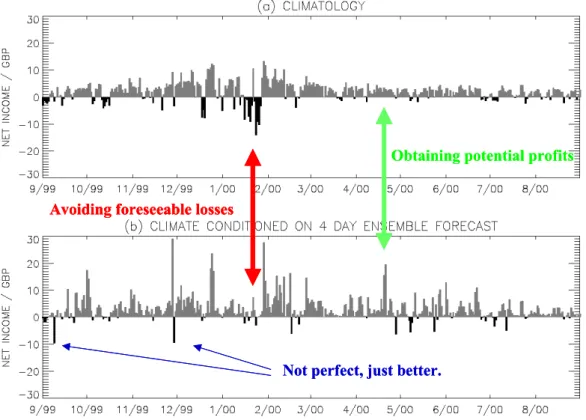
So back to weather roulette: How does the dressed ensemble fare against climatology? Rather well. Consider daily bets, each with a stake of £100, placed over the period of a year starting on December 23, 1999. The three-day forecast based on the ECMWF ensemble made almost £5000 in this period, while the ten day forecast made about £1000 over the same period. As expected even in a perfect model, the value of the ensemble relative to climatology decreases with lead-time. And there is more. The dressed ECMWF ensemble can also be used to bet against house odds based on the (dressed) ECMWF high-resolution best first guess (BFG) forecast. In this case the relative information gain is greater at a lead-time of 10 days than at three, with winnings of over £5000 and over £2000, respectively. This also makes sense, inasmuch as the value of the ensemble forecast relative to climatology is greatest in the short range, while its value relative to a high-resolution forecast is greater at longer lead times (see Roulston and Smith, 2003c for details).
But there is still more, we can contrast the 51 member ensemble with the 10 member ensemble (all ensembles are dressed before use; the best-member kernel will, of course, vary with the size of the ensemble); is there statistically significant value added in the 51 member case relative to case of randomly selecting 10 members? Yes. Relative to the 12-member case? Yes. And the 17-member case? No. Arguably, if Charles were betting only on Heathrow temperatures he would have done as well dressing 17 members as with using (that is, buying) all of them. He would have taken them for free (why not?) but not paid much for them. There is nothing universal about the number 17, in this context. The relevant ensemble size will depend on the details of the target variable as well as the model.
Of course any meteorological sales person worth their salt would immediately point out that users like Charlotte are interested in conditional probabilities of multiple variables at multiple locations. Charlotte is
define fair odds outside PMS as those set by a not-for-profit house aiming only to maintain its endowment while providing a risk management resource (Smith, Judd & Clarke, 2003).
interested in the efficiency of each of her CCGT plants, as well as some integrated measure of electricity demand. But Charles is happy to stick with Heathrow, as long as his probability forecasts are making him money and costing him as little as possible. Making/pricing complicated multi-site derivatives is hard work; and he knows that it is dangerous as well: the curse of dimensionality implies tight constraints on the conditional probability forecasts that can be pulled out of even the best Monte Carlo ensemble with only a few dozen, or a few hundred, members. Charles simply need not take these risks, if the market in trading Heathrow temperatures is both sufficiently profitable and sufficiently liquid. Charlotte, on the other hand, is exposed to these risks; the best she can do is understand the limits placed on the available forecasts by current technology.
There are three important take home messages here: first that, like it or not, the ideal distribution between ensemble size and resolution will be target (that is, user) dependent; second that the marginal value of the n+1st ensemble member will go to zero at different times for different uses; and third that the value of the EPS as a whole will depend critically upon the provision of an archive that allows users to convert these simulations into forecasts of the empirical quantities of interest.
6.
Lies, Damn Lies, and the Perfect Model Scenario
For the materialist, science is what teaches us what to believe. For the empiricist, science is more nearly what teaches us how to give up our beliefs.
Bas van Fraassen Philosophers might call the meteorologist striving for PMS a realist; he believes in the physical reality of the model states and in the truth, or approximate truth, of the model. Alternatively, one modern variety of empiricist aims only for empirical adequacy. Such labels would be inappropriate here, if they were not relevant for the allocation of resources and hence the progress of science.
A model is empirically adequate if the predictions of the model are in agreement with the observations. In this context, the word prediction often refers to prophecies as well as forecasts (see Smith, 1997). To judge empirical adequacy requires some accounting for observational noise and the fair use of a projection operator between the model variables and the observables; i-shadowing would be a necessary condition for empirical adequacy of a dynamical system. There is still much to be understood in this direction, nevertheless it is not clear to me that any of our dynamical models are empirically adequate when applied to dynamic (non-transient) physical systems. There are a number of points, however, where the decision to work within PMS impacts the relevance of the statistics used to judge our models and the choice of how to “improve” them.
6.1
Addressing Model Inadequacy and Multiple Model Ensembles
The philosophical foundations of theories for objective probability distributions are built about the notion of equally likely cases or events (see Giles, 2000). Within PMS, the perfect ensemble is an invocation of this ideal for chaotic dynamical systems that are perfectly modelled but imperfectly observed. This view of the world is available only to our 21st century demon. Given a collection of good but imperfect models, we might try and use them simultaneously to address the issue of model inadequacy. But once we employ multiple imperfect models, the epistemological foundations that justify empirical probability forecasting turn to sand. While we can tolerate uncertainty in the parameter values of a model that comes from the correct model class by invoking what are effectively Bayesian methods, it appears we cannot find an internally consistent framework to support objective probability forecasts8 when using multiple models drawn from distinct model
8 A necessary condition for “objective” as used here is that the forecasts are accountable. This can be tested empirically; we have found no dynamic physical system for which accountable forecasts are available. This is a
classes the union of which is known to be imperfect. Of course one can draw comfort in those aspects of a forecast in which models from each model class independently assign similar probabilities; but only comfort, not confidence (see Smith, 2002). Both systematic and flow dependent differences in the skill scores between the probability forecasts from each model class may help us identify which physical phenomena deserve the most attention in each model class. Thus with time we can improve each of the models in the ensemble, while our probability forecasts remain infinitely remote from the accountable forecasts of our 21st century demon.
6.2
Model Inadequacy and Stochastic Parameterizations
Every attempt at model improvement is an attempt to reduce either parameter uncertainty or model inadequacy. Model inadequacy reflects the fact that there is no model within the class of models available to us that will remain consistent with all the data. For example, there may be no set of parameter values that enable a current model to shadow the observations out-of-sample9 (or even in-sample?). Finding the (metric dependent) “best” parameters, or distributions of parameters, and improving the data assimilation scheme are attempts at minimizing the effects of model inadequacy within a given class of models. But model inadequacy is that which remains even when the best model within the model class is in hand; it affects both stochastic models and deterministic models.
Historically, physicists have tended to employ deterministic models, and operational numerical weather prediction models have been no exception to this trend. There are at least two good reasons why our forecast models should be stochastic in theory. The first comes from recent results (Judd and Smith, 2003) which establish that, given an imperfect nonlinear chaotic model of a deterministic system, better state estimation and better probability forecasts can almost certainly be obtained by using a stochastic model even when the system which generated the data really is deterministic! The second is the persuasive argument that, given current model resolution, it makes much more sense (physically) to employ stochastic subgrid scale parameterisations than to dogmatically employ some mean value, even a good estimate of the expected value (Palmer, 2001). And in addition to these theoretical arguments, stochastic parameterisations have been shown to be better in practice (Buizza et al., 1999).
While adopting stochastic parameterisations will make our models fundamentally stochastic it neither removes the issue of model inadequacy nor makes our model class perfect. Consider what is perhaps the simplest stochastic model for a time series: independent and identically distributed (IID) normal (Gaussian) random variables of mean zero and standard deviation one. Data are numbers. Any data set has a finite (non-zero) probability of coming from this trivial IID model. Adjusting the mean and the standard deviation of the model to equal the observed sample-mean and sample-deviation will make it more difficult to reject the null-hypothesis that our IID “model” generated the data, but not much more difficult. We are soon faced with probabilities so low that, following Borel (1950), we could say with certainty that even a stochastic model does not shadow the observations. The possibility to resemble differs from the ability to shadow.
stronger constraint than other useful meanings of objective probabilities; for example that all “rational men” would converge to the same probability forecast given the same observations and background information. Subjective probability forecasts can, of course, be obtained quite easily from anyone.
9 The phrase out-of-sample reflects the situation where the data used in evaluation were not known before the test was made, in particular that the data was not used in constructing the model or determining parameters. If the same data was used in building the model and testing it, then the test is in-sample. Just as passing an in-sample test is less significant than passing an out-of-sample test, failing an in-sample test is more damning. Note that data are only out-of-sample once.
One often overlooked point here is that whenever we introduce a stochastic element into our models we also introduce an additional constraint: namely that to be a shadowing trajectory, the innovations must be consistent with the stochastic process specified in the model. Stochastic parameterisations may prove a tremendous improvement, but they need not yield i-shadowing trajectories even if there exist some series of innovations that would produce trajectories similar to a time series of analysis states. To be said to shadow, the particular series of innovations must have a reasonable probability given the stochastic process. Experience suggests that it makes little difference if we require a 95% isopleth, or 99%, or 99.999% for that matter. Model inadequacy manifests itself rather robustly Without this additional constraint the application of the concept of i-shadowing to stochastic models would be trivial; the concept would be useless as any rescaled IID process could be said to shadow any set of observations. With this constraint, the introduction of stochastic terms does not guarantee shadowing, and their contribution to improved probability forecasts can be fairly judged.
Even within PMS we must be careful that any critical, theoretically sound assumptions hold if they are relevant in the particular case in question (Gilmour et al. 2001; Hansen and Smith, 2000). Outside PMS a model’s inability to shadow holds implications for operational forecasting, and for the Bayesian paradigm in applied science, if not in mathematics. First of all, it is demonstrable that we can work profitably with imperfect models full of theory-laden (or better still, model-laden10) variables, but we can also be badly misled to misallocate resource in the pursuit of interesting mathematics, which assumes an unjustified level of perfection in our models. Ultimately, only observations can adjudicate this argument. Regardless of what we “know” must be the case.
6.3
Dressing Ensemble Forecasts and the so-called Superensemble
The superensemble method introduced by Krishnamurti et al. (1999) is a very interesting method for extracting a single “locally optimised” BFG forecast from a multi-model ensemble forecast. In short, one finds the optimal weights (in space, time, and target variable) for re-combining an ensemble of multi-model forecasts so as to optimise some root-mean-square skill score of the resulting BFG forecast.
The localised relative skill statistics generated within the “superensemble” approach must contain a wealth of data of value in understanding the shortcomings of each component model and in addressing these model inadequacies. Nevertheless the superensemble approach aspires only to form a single BFG forecast, and thus it might be more aptly called a “superensemble-mean” approach. How might we recast the single forecast output from the “superensemble” approach, in order to make a “like with like” comparison between the “superensemble” output and a probability forecast? The obvious approach would be to dress it, either with some parametric distribution or in the same way we dressed the high-resolution forecasts in section 5 above. Hopefully the shortcoming of either approach is clear: by first forming a single superensemble mean, we have discarded any information in the original distribution of the individual model states. Alternatively, dressing the individual ensemble members retains information from their distribution. So, while it is difficult to see how any “superensemble” approach could outperform either a dressing approach or a product space method (or any other method which retains the distribution information explicitly), it would be interesting to see if in fact there is any relevant information in this distribution!
10 Our theories often involve variables that cannot be fully observed; philosophers would call variables like a temperature field theory-laden. Arguably, this temperature field is something rather different from its in silico realisation in a particular computational model. Thus the model variables composing, say, the T42 temperature “field” might be called model-laden.
6.4
Predicting the relevance of indistinguishable states
The indistinguishable states approach suggests interesting alternatives both to current methods of ensemble formation and to the optimised selection of additional observations. The second are often called adaptive observations since the additional observation that is suggested will vary with the current state of the atmosphere.
Ensemble formation via indistinguishable states avoids the problems of adding finite perturbations to the current best guess analysis. The idea is to direct computational resources towards maintaining a very large ensemble. Rather than discarding ensemble members from the last initialisation they would simply be reweighted as more observations are obtained (see also Beven, 2002). It would relax (that is, discard) the assumptions of linearized uncertainty growth, for example that the observational uncertainty was small relative to the length scale on which the linearisation is relevant (see Hansen and Smith, 2000; Judd, 2003), or that the uncertainty distributions are Gaussian. Of course, an indistinguishable states approach assumes that near shadowing trajectories of reasonable duration do, in fact, exist. Yet if this assumption fails it is difficult to see how the current alternative approaches might function either. Much work remains to be done in terms of quantifying state dependent systematic model error (such as drift, discussed by Orrell et al. 2001) and detecting systematic differences between the behaviour of the analysis and that of the ensemble and its members.
When required, the ensemble would be reseeded from additional trajectories initiated as far back in time as practical, unrealistic perturbations would be identified and discarded without ever being included in a forecast. Reweighting evolved ensemble members given additional data (rather than discarding them), allows larger ensembles to be maintained, and becomes more attractive both as the period between initialising weather ensembles decreases and in the case of seasonal ensembles where many observations may be collected between forecasts launches. In the former case at least, we can form lagged ensemble ensemble forecasts (LEEPS) by reweighting (and perhaps changing the kernel of) older ensemble members if they either remain relevant in light of the current observations or contribute to the probability forecast at any lead-time. Of course, outside PMS the relative weighting and the particular kernel assigned to the elder members can differ from that of the younger members, and it would be interesting to use the time at which this weighting went to zero in estimating an upper bound for a reasonable maximum forecast lead time. Seasonal forecasts as studied within DEMETER (see www.ecmwf.int/demeter) provide ensembles over initial conditions and model structure. While it may prove difficult to argue for maintaining multiple models within PMS, the need to at least sample some structural uncertainties outside PMS provides an a priori
justification for multi-model ensembles, as long as the various models are each plausible. Indeed, it is the use of a single model structure that can only be justified empirically in this case, presumably on the grounds that, given the available alternatives, one model structure is both significantly and consistently better than all the others.
Within PMS, ensembles of indistinguishable states based on shadowing trajectories aims to yield nearly accountable probability forecasts, while operational methods based on singular vector or on bred vector perturbations do not have this aim, even in theory. It also suggests a more flexible approach to adaptive observations if one model simulation (or a set of simulations) was seen to be of particular interest. To identify adaptive observations one can simply divide the current trajectories into two groups, one group in which each member has the interesting property (for example, a major storm) and the other group in which the simulations do not; call these groups red and blue. One could then identify which observations (in space, time, and model-variable) are most likely to provide information distinguishing the distribution of red trajectories from the distribution of blue, or better said: which observations are most likely to give members of one of the groups high probability and those of the other low probability. As additional regular
observations are obtained, the main computational overhead in updating our method is to reweight the existing trajectories, a relatively low computational cost and an advantage with respect to alternative approaches (see Hansen and Smith, 2001, and references thereof).
With multi-model forecasts we can also use the indistinguishable states framework to select observations that are most likely to falsify one of two models. To paraphrase John Wheeler: Each of our models is false; the trick is to falsify them as quickly as possible. Here only the observations can adjudicate; while what we decide to measure is constrained by what we can think of measuring, the measurement obtained is not. Le Verrier was as confident of his prediction of Vulcan as he was of his prediction of Neptune, and while both were observed for some time only Neptune is with us today.
Just as the plural of datum is not information, the plural of good idea is not theoretical framework. The indistinguishable states approach to forecasting and predictability has significant strengths over competing strategies, but its operational relevance faces a number of hurdles that have yet to be cleared. This statement should not be taken to indicate that the competition has cleared them cleanly!
6.5
A short digression toward longer time scales: the in-sample science
Given the comments made in the earlier talks by Tim Palmer and Myles Allen, we will not resist a short digression towards longer time scales. An operational weather model makes many 7-day forecasts over its short lifetime; contrast this case with that of a climate model used to make 50-year forecasts, yet considered obsolete within a year or two. The continuous feedback from making forecasts on new unseen (out-of-sample) data is largely denied the climate modeller, who is constrained by the nature of the problem to forever violate one of the first maxims of undergraduate statistics: never restrict your analysis to in-sample statistics. By construction, climate modelling is an in-sample science. And the fundamentally transient nature of problem makes it harder still.
As argued elsewhere (Smith, 2002), an in-sample science requires a different kind of consistency constraint. If model inadequacy foils our attempts at objective probability forecasts within the weather scenario, there is little if any chance of recovering these in the climate scenario11. We can, however, interpret multiple models in a different way. While approaches like best-member dressing can take into account the fact that different models will perform better in different conditions in the weather context, a climate modeller cannot exploit such observations. In the weather scenario we can use all information available at the time the models are launched when interpreting the distribution of model simulations, and as we launch (at least) once a day, we can learn from our mistakes.
Inasmuch as climate forecasting is a transient experiment, we launch only once. It is not clear how one might combine a collection of single runs of different climate models into a sensible probability forecast. But by studying the in-sample behaviour of ensembles under a variety of models, we can tune each model until an ensemble of initial conditions under each and every individual model can at least bound the in-sample observations, say from 1950 to 2000. If ensembles are then run into the future, we can look for the variables (space and time scales) on which the individual model ensembles bound the past and agree (in distribution) regarding the future.
Of course agreement does not ensure relevance to the future; our collection of models can share a common flaw. But if differences in the subtle details of different models that have similar (plausible) in-sample performance are shown to yield significantly different forecast distributions, then no coherent picture
11 I would have said no chance, but Myles Allen argues effectively that climate models might provide information on “climate variables” without accurately resolving detailed aspects of the Earth System.