Massive Online Analysis Manual

Massive Online

Analysis

Manual

Albert Bifet, Richard Kirkby,

Philipp Kranen, Peter Reutemann

Contents

1 Introduction 1

1.1 Data streams Evaluation . . . 2

2 Installation 5 2.1 WEKA . . . 6

3 Using MOA 7 3.1 Using the GUI . . . 7

3.1.1 Classification . . . 7

3.1.2 Regression . . . 8

3.1.3 Clustering . . . 8

3.2 Using the command line . . . 12

3.2.1 Comparing two classifiers . . . 14

4 Using the API 17 4.1 Creating a new classifier . . . 17

4.2 Compiling a classifier. . . 22 5 Tasks in MOA 25 5.1 WriteStreamToARFFFile . . . 25 5.2 MeasureStreamSpeed . . . 25 5.3 LearnModel. . . 26 5.4 EvaluateModel. . . 26 5.5 EvaluatePeriodicHeldOutTest . . . 27 5.6 EvaluateInterleavedTestThenTrain. . . 27 5.7 EvaluatePrequential . . . 28 5.8 EvaluateInterleavedChunks . . . 29

6 Evolving data streams 31 6.1 Streams . . . 31 6.1.1 ArffFileStream . . . 31 6.1.2 ConceptDriftStream . . . 32 6.1.3 ConceptDriftRealStream . . . 33 6.1.4 FilteredStream . . . 34 6.1.5 AddNoiseFilter . . . 34 6.2 Streams Generators . . . 34 6.2.1 generators.AgrawalGenerator . . . 34 6.2.2 generators.HyperplaneGenerator . . . 35 6.2.3 generators.LEDGenerator. . . 36

6.2.4 generators.LEDGeneratorDrift . . . 36 6.2.5 generators.RandomRBFGenerator . . . 37 6.2.6 generators.RandomRBFGeneratorDrift . . . 37 6.2.7 generators.RandomTreeGenerator . . . 38 6.2.8 generators.SEAGenerator. . . 39 6.2.9 generators.STAGGERGenerator . . . 39 6.2.10 generators.WaveformGenerator . . . 40 6.2.11 generators.WaveformGeneratorDrift . . . 40 7 Classifiers 41 7.1 Bayesian Classifiers . . . 42 7.1.1 NaiveBayes . . . 42 7.1.2 NaiveBayesMultinomial. . . 42 7.2 Decision Trees . . . 43 7.2.1 DecisionStump . . . 43 7.2.2 HoeffdingTree. . . 43 7.2.3 HoeffdingOptionTree . . . 45 7.2.4 HoeffdingAdaptiveTree . . . 47 7.2.5 AdaHoeffdingOptionTree . . . 47 7.3 Meta Classifiers . . . 47 7.3.1 OzaBag . . . 47 7.3.2 OzaBoost. . . 48 7.3.3 OCBoost . . . 48 7.3.4 OzaBagASHT . . . 49 7.3.5 OzaBagADWIN . . . 50 7.3.6 AccuracyWeightedEnsemble . . . 51 7.3.7 AccuracyUpdatedEnsemble . . . 52 7.3.8 LimAttClassifier. . . 52 7.3.9 LeveragingBag . . . 53 7.4 Function Classifiers . . . 54 7.4.1 MajorityClass . . . 54 7.4.2 Perceptron . . . 54 7.4.3 SGD . . . 54 7.4.4 SPegasos . . . 54 7.5 Drift Classifiers. . . 55 7.5.1 SingleClassifierDrift . . . 55

8 Bi-directional interface with WEKA 57 8.1 WEKA classifiers from MOA . . . 57

8.1.1 WekaClassifier . . . 58

CONTENTS

1

Introduction

Massive Online Analysis (MOA) is a software environment for implementing algorithms and running experiments for online learning from evolving data streams. MOA is designed to deal with the challenging problems of scaling up the implementation of state of the art algorithms to real world dataset sizes and of making algorithms comparable in benchmark streaming settings.

MOA contains a collection of offline and online algorithms for both classifi-cation and clustering as well as tools for evaluation. Researchers benefit from MOA by getting insights into workings and problems of different approaches, practitioners can easily compare several algorithms and apply them to real world data sets and settings.

MOA supports bi-directional interaction with WEKA, the Waikato Environ-ment for Knowledge Analysis, which is an award-winning open-source work-bench containing implementations of a wide range of batch machine learning methods. WEKA is also written in Java. The main benefits of Java are porta-bility, where applications can be run on any platform with an appropriate Java virtual machine, and the strong and well-developed support libraries. Use of the language is widespread, and features such as the automatic garbage col-lection help to reduce programmer burden and error.

One of the key data structures used in MOA is the description of an exam-ple from a data stream. This structure borrows from WEKA, where an examexam-ple is represented by an array of double precision floating point values. This pro-vides freedom to store all necessary types of value – numeric attribute values can be stored directly, and discrete attribute values and class labels are repre-sented by integer index values that are stored as floating point values in the

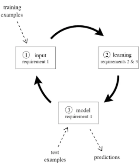
Figure 1.1: The data stream classification cycle

array. Double precision floating point values require storage space of 64 bits, or 8 bytes. This detail can have implications for memory usage.

1.1 Data streams Evaluation

A data stream environment has different requirements from the traditional setting. The most significant are the following:

Requirement 1 Process an example at a time, and inspect it only once (at most)

Requirement 2 Use a limited amount of memory Requirement 3 Work in a limited amount of time Requirement 4 Be ready to predict at any time

We have to consider these requirements in order to design a new experimental framework for data streams. Figure 1.1 illustrates the typical use of a data stream classification algorithm, and how the requirements fit in a repeating cycle:

1.1. DATA STREAMS EVALUATION

1. The algorithm is passed the next available example from the stream (re-quirement 1).

2. The algorithm processes the example, updating its data structures. It does so without exceeding the memory bounds set on it (requirement 2), and as quickly as possible (requirement 3).

3. The algorithm is ready to accept the next example. On request it is able to predict the class of unseen examples (requirement 4).

In traditional batch learning the problem of limited data is overcome by an-alyzing and averaging multiple models produced with different random ar-rangements of training and test data. In the stream setting the problem of (effectively) unlimited data poses different challenges. One solution involves taking snapshots at different times during the induction of a model to see how much the model improves.

The evaluation procedure of a learning algorithm determines which exam-ples are used for training the algorithm, and which are used to test the model output by the algorithm. The procedure used historically in batch learning has partly depended on data size. As data sizes increase, practical time limitations prevent procedures that repeat training too many times. It is commonly ac-cepted with considerably larger data sources that it is necessary to reduce the numbers of repetitions or folds to allow experiments to complete in reasonable time. When considering what procedure to use in the data stream setting, one of the unique concerns is how to build a picture of accuracy over time. Two main approaches arise:

• Holdout: When traditional batch learning reaches a scale where cross-validation is too time consuming, it is often accepted to instead measure performance on a single holdout set. This is most useful when the di-vision between train and test sets have been pre-defined, so that results from different studies can be directly compared.

• Interleaved Test-Then-Train or Prequential: Each individual example can be used to test the model before it is used for training, and from this the accuracy can be incrementally updated. When intentionally per-formed in this order, the model is always being tested on examples it has not seen. This scheme has the advantage that no holdout set is needed for testing, making maximum use of the available data. It also ensures a smooth plot of accuracy over time, as each individual example will become increasingly less significant to the overall average.

As data stream classification is a relatively new field, such evaluation practices are not nearly as well researched and established as they are in the traditional batch setting. The majority of experimental evaluations use less than one mil-lion training examples. In the context of data streams this is disappointing, because to be truly useful at data stream classification the algorithms need to be capable of handling very large (potentially infinite) streams of examples. Demonstrating systems only on small amounts of data does not build a con-vincing case for capacity to solve more demanding data stream applications.

MOA permits adequately evaluate data stream classification algorithms on large streams, in the order of tens of millions of examples where possible, and under explicit memory limits. Any less than this does not actually test algorithms in a realistically challenging setting.

2

Installation

The following manual is based on a Unix/Linux system with Java 6 SDK or greater installed. Other operating systems such as Microsoft Windows will be similar but may need adjustments to suit.

MOA needs the following files:

•

moa.jar

•

sizeofag.jar

They are available from

•

http://sourceforge.net/projects/moa-datastream/

•

http://www.jroller.com/resources/m/maxim/sizeofag.jar

These files are needed to run the MOA software from the command line:

java -Xmx4G -cp moa.jar -javaagent:sizeofag.jar moa.DoTask \

LearnModel -l DecisionStump \

-s generators.WaveformGenerator \

-m 1000000 -O model1.moa

and the graphical interface:

java -Xmx4G -cp moa.jar -javaagent:sizeofag.jar moa.gui.GUI

Xmx4G

increases the maximum heap size to 4GB for your java engine, as

2.1 WEKA

It is possible to use the classifiers available in WEKA 3.7. The file

weka.jar

is available from

http://sourceforge.net/projects/weka/files/weka-3-7/

This file is needed to run the MOA software with WEKA from the command line:

java -Xmx4G -cp moa.jar:weka.jar -javaagent:sizeofag.jar

moa.DoTask "LearnModel \

-l (WekaClassifier -l weka.classifiers.trees.J48) \

-s generators.WaveformGenerator -m 1000000 -O model1.moa"

and the graphical interface:

java -Xmx4G -cp moa.jar:weka.jar -javaagent:sizeofag.jar \

moa.gui.GUI

or, using Microsoft Windows:

java -Xmx4G -cp moa.jar;weka.jar -javaagent:sizeofag.jar

moa.DoTask "LearnModel

-l (WekaClassifier -l weka.classifiers.trees.J48)

-s generators.WaveformGenerator -m 1000000 -O model1.moa"

java -Xmx4G -cp moa.jar;weka.jar -javaagent:sizeofag.jar

3

Using MOA

3.1 Using the GUI

A graphical user interface for configuring and running tasks is available with the command:

java -Xmx4G -cp moa.jar -javaagent:sizeofag.jar moa.gui.GUI

There are two main tabs: one for classification and one for clustering.

3.1.1

Classification

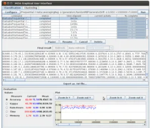
Figure 3.1: Graphical user interface of MOA

Click ’Configure’ to set up a task, when ready click to launch a task click ’Run’. Several tasks can be run concurrently. Click on different tasks in the list and control them using the buttons below. If textual output of a task is

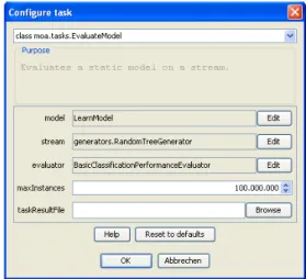
Figure 3.2: Options to set up a task in MOA

available it will be displayed in the bottom half of the GUI, and can be saved to disk.

Note that the command line text box displayed at the top of the window represents textual commands that can be used to run tasks on the command line as described in the next chapter. The text can be selected then copied onto the clipboard. In the bottom of the GUI there is a graphical display of the results. It is possible to compare the results of two different tasks: the current task is displayed in red, and the selected previously is in blue.

3.1.2

Regression

It is now possible to run regression evaluations using the evaluators

•

BasicRegressionPerformanceEvaluator

•

WindowRegressionPerformanceEvaluator

Currently, it is only possible to use the regressors in the IBLStreams extension of MOA or in WEKA. See Section2.1and Chapter8for more information how to use WEKA learners.

3.1.3

Clustering

The stream clustering tab of MOA has the following main components:

• data generators for stream clustering on evolving streams (including events like novelty, merge, etc.),

3.1. USING THE GUI

Figure 3.3: Option dialog for the RBF data generator (by storing and loading settings benchmark streaming data sets can be shared for repeatability and comparison).

• a set of state-of-the-art stream clustering algorithms, • evaluation measures for stream clustering,

• visualization tools for analyzing results and comparing different settings. Data feeds and data generators

Figure 3.3 shows a screenshot of the configuration dialog for the RBF data generator with events. Generally the dimensionality, number and size of clus-ters can be set as well as the drift speed, decay horizon (aging) and noise rate etc. Events constitute changes in the underlying data model such as growing of clusters, merging of clusters or creation of new clusters. Using the event frequency and the individual event weights, one can study the behaviour and performance of different approaches on various settings. Finally, the settings for the data generators can be stored and loaded, which offers the opportunity of sharing settings and thereby providing benchmark streaming data sets for repeatability and comparison.

Stream clustering algorithms

Currently MOA contains several stream clustering methods including:

• StreamKM++: It computes a small weighted sample of the data stream and it uses the k-means++ algorithm as a randomized seeding tech-nique to choose the first values for the clusters. To compute the small sample, it employs coreset constructions using a coreset tree for speed up.

• CluStream: It maintains statistical information about the data using micro-clusters. These micro-clusters are temporal extensions of clus-ter feature vectors. The micro-clusclus-ters are stored at snapshots in time following a pyramidal pattern. This pattern allows to recall summary statistics from different time horizons.

• ClusTree: It is a parameter free algorithm automatically adapting to the speed of the stream and it is capable of detecting concept drift, novelty, and outliers in the stream. It uses a compact and self-adaptive index structure for maintaining stream summaries.

• Den-Stream: It uses dense micro-clusters (named core-micro-cluster) to summarize clusters. To maintain and distinguish the potential clusters and outliers, this method presents core-cluster and outlier micro-cluster structures.

• CobWeb. One of the first incremental methods for clustering data. It uses a classification tree. Each node in a classification tree represents a class (concept) and is labeled by a probabilistic concept that summarizes the attribute-value distributions of objects classified under the node. Visualization and analysis

After the evaluation process is started, several options for analyzing the out-puts are given:

• the stream can be stopped and the current (micro) clustering result can be passed as a data set to the WEKA explorer for further analysis or mining;

• the evaluation measures, which are taken at configurable time intervals, can be stored as a .csv file to obtain graphs and charts offline using a program of choice;

3.1. USING THE GUI

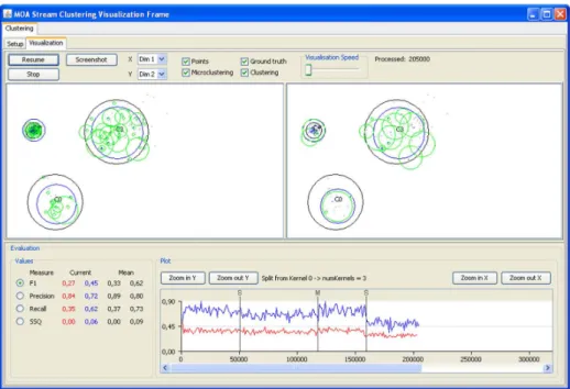
Figure 3.4: Visualization tab of the clustering MOA graphical user interface. • last but not least both the clustering results and the corresponding

mea-sures can be visualized online within MOA.

MOA allows the simultaneous configuration and evaluation of two differ-ent setups for direct comparison, e.g. of two differdiffer-ent algorithms on the same stream or the same algorithm on streams with different noise levels etc.

The visualization component allows to visualize the stream as well as the clustering results, choose dimensions for multi dimensional settings, and com-pare experiments with different settings in parallel. Figure3.4shows a screen shot of the visualization tab. For this screen shot two different settings of the CluStream algorithm were compared on the same stream setting (including merge/split events every 50000 examples) and four measures were chosen for online evaluation (F1, Precision, Recall, and SSQ).

The upper part of the GUI offers options to pause and resume the stream, adjust the visualization speed, choose the dimensions for x and y as well as the components to be displayed (points, micro- and macro clustering and ground truth). The lower part of the GUI displays the measured values for both set-tings as numbers (left side, including mean values) and the currently selected measure as a plot over the arrived examples (right, F1 measure in this exam-ple). For the given setting one can see a clear drop in the performance after the split event at roughly 160000 examples (event details are shown when

choosing the corresponding vertical line in the plot). While this holds for both settings, the left configuration (red, CluStream with 100 micro clusters) is constantly outperformed by the right configuration (blue, CluStream with 20 micro clusters).

3.2 Using the command line

In this section we are going to show some examples of tasks performed using the command line.

The first example will command MOA to train the

HoeffdingTree

classi-fier and create a model. The

moa.DoTask

class is the main class for running tasks on the command line. It will accept the name of a task followed by any appropriate parameters. The first task used is the

LearnModel

task. The

-l

parameter specifies the learner, in this case the

HoeffdingTree

class. The

-s

parameter specifies the data stream to learn from, in this case it is specified

generators.WaveformGenerator

, which is a data stream generator that

produces a three-class learning problem of identifying three types of wave-form. The

-m

option specifies the maximum number of examples to train the learner with, in this case one million examples. The

-O

option specifies a file to output the resulting model to:

java -cp moa.jar -javaagent:sizeofag.jar moa.DoTask \ LearnModel -l trees.HoeffdingTree \

-s generators.WaveformGenerator -m 1000000 -O model1.moa

This will create a file named

model1.moa

that contains the decision stump model that was induced during training.

The next example will evaluate the model to see how accurate it is on a set of examples that are generated using a different random seed. The

EvaluateModel

task is given the parameters needed to load the model

pro-duced in the previous step, generate a new waveform stream with a random seed of 2, and test on one million examples:

java -cp moa.jar -javaagent:sizeofag.jar moa.DoTask \ "EvaluateModel -m file:model1.moa \

-s (generators.WaveformGenerator -i 2) -i 1000000"

This is the first example of nesting parameters using brackets. Quotes have been added around the description of the task, otherwise the operating system may be confused about the meaning of the brackets.

3.2. USING THE COMMAND LINE

classified instances = 1,000,000

classifications correct (percent) = 84.474 Kappa Statistic (percent) = 76.711

Note the the above two steps can be achieved by rolling them into one, avoiding the need to create an external file, as follows:

java -cp moa.jar -javaagent:sizeofag.jar moa.DoTask \ "EvaluateModel -m (LearnModel -l trees.HoeffdingTree \ -s generators.WaveformGenerator -m 1000000) \

-s (generators.WaveformGenerator -i 2) -i 1000000"

The task

EvaluatePeriodicHeldOutTest

will train a model while tak-ing snapshots of performance ustak-ing a held-out test set at periodic intervals. The following command creates a comma separated values file, training the

HoeffdingTree

classifier on the

WaveformGenerator

data, using the first

100 thousand examples for testing, training on a total of 100 million examples, and testing every one million examples:

java -cp moa.jar -javaagent:sizeofag.jar moa.DoTask \ "EvaluatePeriodicHeldOutTest -l trees.HoeffdingTree \ -s generators.WaveformGenerator \

-n 100000 -i 100000000 -f 1000000" > dsresult.csv

For the purposes of comparison, a bagging learner using ten decisions trees can be trained on the same problem:

java -cp moa.jar -javaagent:sizeofag.jar moa.DoTask \

"EvaluatePeriodicHeldOutTest -l (OzaBag -l trees.HoeffdingTree -s 10)\ -s generators.WaveformGenerator \

-n 100000 -i 100000000 -f 1000000" > htresult.csv

Another evaluation method implemented in MOA is Interleaved Test-Then-TrainorPrequential: Each individual example is used to test the model before it is used for training, and from this the accuracy is incrementally updated. When intentionally performed in this order, the model is always being tested on examples it has not seen. This scheme has the advantage that no holdout set is needed for testing, making maximum use of the available data. It also ensures a smooth plot of accuracy over time, as each individual example will become increasingly less significant to the overall average.

An example of the EvaluateInterleavedTestThenTrain task creating a comma separated values file, training the HoeffdingTree classifier on the Waveform-Generator data, training and testing on a total of 100 million examples, and testing every one million examples, is the following:

java -cp moa.jar -javaagent:sizeofag.jar moa.DoTask \

"EvaluateInterleavedTestThenTrain -l trees.HoeffdingTree \ -s generators.WaveformGenerator \

3.2.1

Comparing two classifiers

Suppose we would like to compare the learning curves of a decision stump and a Hoeffding Tree. First, we will execute the task

EvaluatePeriodicHeldOutTest

to train a model while taking snapshots of performance using a held-out test set at periodic intervals. The following commands create comma separated valuesfiles, training the

DecisionStump

and the

HoeffdingTree

classifier on the

WaveformGenerator

data, using the first 100 thousand examples for testing, training on a total of 100 million examples, and testing every one million examples:

java -cp moa.jar -javaagent:sizeofag.jar moa.DoTask \ "EvaluatePeriodicHeldOutTest -l trees.DecisionStump \ -s generators.WaveformGenerator \

-n 100000 -i 100000000 -f 1000000" > dsresult.csv

java -cp moa.jar -javaagent:sizeofag.jar moa.DoTask \ "EvaluatePeriodicHeldOutTest -l trees.HoeffdingTree \ -s generators.WaveformGenerator \

-n 100000 -i 100000000 -f 1000000" > htresult.csv

Assuming that

gnuplot

is installed on the system, the learning curves can be plotted with the following commands:

gnuplot> set datafile separator "," gnuplot> set ylabel "% correct"

gnuplot> set xlabel "examples processed" gnuplot> plot [][0:100] \

"dsresult.csv" using 1:9 with linespoints \ title "DecisionStumpTutorial", \

"htresult.csv" using 1:9 with linespoints \ title "HoeffdingTree"

3.2. USING THE COMMAND LINE 0 20 40 60 80 100

1e+06 2e+06 3e+06 4e+06 5e+06 6e+06 7e+06 8e+06 9e+06 1e+07

% correct

examples processed

DecisionStumpTutorial HoeffdingTree

For this problem it is obvious that a full tree can achieve higher accuracy than a single stump, and that a stump has very stable accuracy that does not improve with further training.

4

Using the API

It’s easy to use the methods of MOA inside Java Code. For example, this is the Java code for a prequential evaluation:

Listing 4.1: Java Code Example

1 i n t numInstances=10000; 2

3 C l a s s i f i e r l e a r n e r=new H o e f f d i n g T r e e ( ) ;

4 RandomRBFGenerator stream=new RandomRBFGenerator ( ) ; 5 stream . p r e p a r e F o r U s e ( ) ; 6 7 l e a r n e r . s e t M o d e l C o n t e x t ( stream . getHeader ( ) ) ; 8 l e a r n e r . p r e p a r e F o r U s e ( ) ; 9 10 i n t numberSamplesCorrect=0; 11 i n t numberSamples=0; 12 boolean i s T e s t i n g=t r u e;

13 while( stream . h a s M o r e I n s t a n c e s ( ) && numberSamples<numInstances ){

14 I n s t a n c e t r a i n I n s t =stream . n e x t I n s t a n c e ( ) ; 15 i f( i s T e s t i n g ){ 16 i f( l e a r n e r . c o r r e c t l y C l a s s i f i e s ( t r a i n I n s t ) ){ 17 numberSamplesCorrect++; 18 } 19 } 20 numberSamples++; 21 l e a r n e r . t r a i n O n I n s t a n c e ( t r a i n I n s t ) ; 22 }

23 double a c c u r a c y =100.0∗(double) numberSamplesCorrect / (double) numberSamples ; 24 System . out . p r i n t l n ( numberSamples+" i n s t a n c e s p r o c e s s e d with "+a c c u r a c y+"% a c c u r a c y " ) ;

4.1 Creating a new classifier

To demonstrate the implementation and operation of learning algorithms in the system, the Java code of a simple decision stump classifier is studied. The classifier monitors the result of splitting on each attribute and chooses the attribute the seems to best separate the classes, based on information gain. The decision is revisited many times, so the stump has potential to change over time as more examples are seen. In practice it is unlikely to change after sufficient training.

To describe the implementation, relevant code fragments are discussed in turn, with the entire code listed (Listing 4.8) at the end. The line numbers from the fragments match up with the final listing.

A simple approach to writing a classifier is to extend

moa.classifiers.AbstractClassifier

(line 10), which will take care of

certain details to ease the task.

Listing 4.2: Option handling

14 p u b l i c I n t O p t i o n g r a c e P e r i o d O p t i o n =new I n t O p t i o n ( " g r a c e P e r i o d " , ’ g ’ , 15 " The number o f i n s t a n c e s t o o b s e r v e between model changes . " , 16 1000 , 0 , I n t e g e r . MAX_VALUE ) ; 17 18 p u b l i c F l a g O p t i o n b i n a r y S p l i t s O p t i o n=new F l a g O p t i o n ( " b i n a r y S p l i t s " , ’ b ’ , 19 " Only a l l o w b i n a r y s p l i t s . " ) ; 20 21 p u b l i c C l a s s O p t i o n s p l i t C r i t e r i o n O p t i o n =new C l a s s O p t i o n ( " s p l i t C r i t e r i o n " , 22 ’ c ’ , " S p l i t c r i t e r i o n t o use . " , S p l i t C r i t e r i o n .c l a s s, 23 " I n f o G a i n S p l i t C r i t e r i o n " ) ;

To set up the public interface to the classifier, the options available to the user must be specified. For the system to automatically take care of option handling, the options need to be public members of the class, that extend the

moa.options.Option

type.

The decision stump classifier example has three options, each of a different type. The meaning of the first three parameters used to construct options are consistent between different option types. The first parameter is a short name used to identify the option. The second is a character intended to be used on the command line. It should be unique—a command line character cannot be repeated for different options otherwise an exception will be thrown. The third standard parameter is a string describing the purpose of the option. Additional parameters to option constructors allow things such as default values and valid ranges to be specified.

The first option specified for the decision stump classifier is the “grace pe-riod”. The option is expressed with an integer, so the option has the type

IntOption

. The parameter will control how frequently the best stump is

reconsidered when learning from a stream of examples. This increases the efficiency of the classifier—evaluating after every single example is expensive, and it is unlikely that a single example will change the decision of the current best stump. The default value of 1000 means that the choice of stump will be re-evaluated only after 1000 examples have been observed since the last evaluation. The last two parameters specify the range of values that are al-lowed for the option—it makes no sense to have a negative grace period, so the range is restricted to integers 0 or greater.

The second option is a flag, or a binary switch, represented by a

FlagOption

. By default all flags are turned off, and will be turned on only

when a user requests so. This flag controls whether the decision stumps should only be allowed to split two ways. By default the stumps are allowed have more than two branches.

The third option determines the split criterion that is used to decide which stumps are the best. This is a

ClassOption

that requires a particular Java

4.1. CREATING A NEW CLASSIFIER

class of the type

SplitCriterion

. If the required class happens to be an

OptionHandler

then those options will be used to configure the object that

is passed in.

Listing 4.3: Miscellaneous fields

25 p ro te ct ed A t t r i b u t e S p l i t S u g g e s t i o n b e s t S p l i t ; 26 27 p ro te ct ed D o u b l e V e c t o r o b s e r v e d C l a s s D i s t r i b u t i o n ; 28 29 p ro te ct ed AutoExpandVector<A t t r i b u t e C l a s s O b s e r v e r>a t t r i b u t e O b s e r v e r s ; 30 31 p ro te ct ed double w e i g h t S e e n A t L a s t S p l i t ; 32 33 p u b l i c boolean i s R a n d o m i z a b l e ( ) { 34 return f a l s e; 35 }

Four global variables are used to maintain the state of the classifier.

The

bestSplit

field maintains the current stump that has been chosen by

the classifier. It is of type

AttributeSplitSuggestion

, a class used to split instances into different subsets.

The

observedClassDistribution

field remembers the overall

distri-bution of class labels that have been observed by the classifier. It is of type

DoubleVector

, which is a handy class for maintaining a vector of floating

point values without having to manage its size.

The

attributeObservers

field stores a collection of

AttributeClassObserver

s, one for each attribute. This is the information

needed to decide which attribute is best to base the stump on.

The

weightSeenAtLastSplit

field records the last time an evaluation

was performed, so that it can be determined when another evaluation is due, depending on the grace period parameter.

The

isRandomizable()

function needs to be implemented to specify

whether the classifier has an element of randomness. If it does, it will au-tomatically be set up to accept a random seed. This classifier is does not, so

false

is returned.

Listing 4.4: Preparing for learning

37 @Override 38 p u b l i c void r e s e t L e a r n i n g I m p l ( ) { 39 t h i s. b e s t S p l i t=n u l l; 40 t h i s. o b s e r v e d C l a s s D i s t r i b u t i o n=new D o u b l e V e c t o r ( ) ; 41 t h i s. a t t r i b u t e O b s e r v e r s=newAutoExpandVector<A t t r i b u t e C l a s s O b s e r v e r>(); 42 t h i s. w e i g h t S e e n A t L a s t S p l i t= 0 . 0 ; 43 }

This function is called before any learning begins, so it should set the de-fault state when no information has been supplied, and no training examples have been seen. In this case, the four global fields are set to sensible defaults.

Listing 4.5: Training on examples

45 @Override

46 p u b l i c void t r a i n O n I n s t a n c e I m p l ( I n s t a n c e i n s t ) {

48 . weight ( ) ) ; 49 f o r (i n t i =0 ; i < i n s t . n u m A t t r i b u t e s ( )−1 ; i++){ 50 i n t i n s t A t t I n d e x=m o d e l A t t I n d e x T o I n s t a n c e A t t I n d e x ( i , i n s t ) ; 51 A t t r i b u t e C l a s s O b s e r v e r obs= t h i s. a t t r i b u t e O b s e r v e r s . g e t ( i ) ; 52 i f ( obs==n u l l) { 53 obs=i n s t . a t t r i b u t e ( i n s t A t t I n d e x ) . i s N o m i n a l ( ) ? 54 newNominalClassObserver ( ) : newNumericClassObserver ( ) ; 55 t h i s. a t t r i b u t e O b s e r v e r s . s e t ( i , obs ) ; 56 } 57 obs . o b s e r v e A t t r i b u t e C l a s s ( i n s t . v a l u e ( i n s t A t t I n d e x ) , (i n t) i n s t 58 . c l a s s V a l u e ( ) , i n s t . weight ( ) ) ; 59 } 60 i f (t h i s. trainingWeightSeenByModel− t h i s. w e i g h t S e e n A t L a s t S p l i t>= 61 t h i s. g r a c e P e r i o d O p t i o n . g e t V a l u e ( ) ) { 62 t h i s. b e s t S p l i t= f i n d B e s t S p l i t ( ( S p l i t C r i t e r i o n ) 63 g e t P r e p a r e d C l a s s O p t i o n (t h i s. s p l i t C r i t e r i o n O p t i o n ) ) ; 64 t h i s. w e i g h t S e e n A t L a s t S p l i t= t h i s. trainingWeightSeenByModel ; 65 } 66 }

This is the main function of the learning algorithm, called for every training example in a stream. The first step, lines 47-48, updates the overall recorded distribution of classes. The loop from line 49 to line 59 repeats for every attribute in the data. If no observations for a particular attribute have been seen previously, then lines 53-55 create a new observing object. Lines 57-58 update the observations with the values from the new example. Lines 60-61 check to see if the grace period has expired. If so, the best split is re-evaluated.

Listing 4.6: Functions used during training

79 pr ot ec te d A t t r i b u t e C l a s s O b s e r v e r newNominalClassObserver ( ) { 80 return new N o m i n a l A t t r i b u t e C l a s s O b s e r v e r ( ) ; 81 } 82 83 pr ot ec te d A t t r i b u t e C l a s s O b s e r v e r newNumericClassObserver ( ) { 84 return new G a u s s i a n N u m e r i c A t t r i b u t e C l a s s O b s e r v e r ( ) ; 85 } 86 87 pr ot ec te d A t t r i b u t e S p l i t S u g g e s t i o n f i n d B e s t S p l i t ( S p l i t C r i t e r i o n c r i t e r i o n ) { 88 A t t r i b u t e S p l i t S u g g e s t i o n bestFound=n u l l; 89 double b e s t M e r i t=Double . NEGATIVE_INFINITY ;

90 double[] p r e S p l i t D i s t =t h i s. o b s e r v e d C l a s s D i s t r i b u t i o n . getArrayCopy ( ) ; 91 f o r (i n t i =0 ; i < t h i s. a t t r i b u t e O b s e r v e r s . s i z e ( ) ; i++){ 92 A t t r i b u t e C l a s s O b s e r v e r obs= t h i s. a t t r i b u t e O b s e r v e r s . g e t ( i ) ; 93 i f ( obs != n u l l) { 94 A t t r i b u t e S p l i t S u g g e s t i o n s u g g e s t i o n = 95 obs . g e t B e s t E v a l u a t e d S p l i t S u g g e s t i o n ( 96 c r i t e r i o n , 97 p r e S p l i t D i s t , 98 i , 99 t h i s. b i n a r y S p l i t s O p t i o n . i s S e t ( ) ) ; 100 i f ( s u g g e s t i o n . m e r i t> b e s t M e r i t ) { 101 b e s t M e r i t =s u g g e s t i o n . m e r i t ; 102 bestFound=s u g g e s t i o n ; 103 } 104 } 105 } 106 return bestFound ; 107 }

These functions assist the training algorithm.

newNominalClassObserver

and

newNumericClassObserver

are

respon-sible for creating new observer objects for nominal and numeric attributes, respectively. The

findBestSplit()

function will iterate through the possi-ble stumps and return the one with the highest ‘merit’ score.

Listing 4.7: Predicting class of unknown examples

4.1. CREATING A NEW CLASSIFIER 69 i f (t h i s. b e s t S p l i t != n u l l) { 70 i n t branch=t h i s. b e s t S p l i t . s p l i t T e s t . b r a n c h F o r I n s t a n c e ( i n s t ) ; 71 i f ( branch>=0) { 72 return t h i s. b e s t S p l i t 73 . r e s u l t i n g C l a s s D i s t r i b u t i o n F r o m S p l i t ( branch ) ; 74 } 75 } 76 return t h i s. o b s e r v e d C l a s s D i s t r i b u t i o n . getArrayCopy ( ) ; 77 }

This is the other important function of the classifier besides training—using the model that has been induced to predict the class of examples. For the de-cision stump, this involves calling the functions

branchForInstance()

and

resultingClassDistributionFromSplit()

that are implemented by the

AttributeSplitSuggestion

class.

Putting all of the elements together, the full listing of the tutorial class is given below.

Listing 4.8: Full listing

1 package moa . c l a s s i f i e r s ; 2

3 importmoa . c o r e . AutoExpandVector ; 4 importmoa . c o r e . D o u b l e V e c t o r ; 5 importmoa . o p t i o n s . C l a s s O p t i o n ; 6 importmoa . o p t i o n s . F l a g O p t i o n ; 7 importmoa . o p t i o n s . I n t O p t i o n ; 8 importweka . c o r e . I n s t a n c e ; 9 10 p u b l i c c l a s s D e c i s i o n S t u m p T u t o r i a l extends A b s t r a c t C l a s s i f i e r { 11 12 p r i v a t e s t a t i c f i n a l long s e r i a l V e r s i o n U I D =1L ; 13 14 p u b l i c I n t O p t i o n g r a c e P e r i o d O p t i o n =new I n t O p t i o n ( " g r a c e P e r i o d " , ’ g ’ , 15 " The number o f i n s t a n c e s t o o b s e r v e between model changes . " , 16 1000 , 0 , I n t e g e r . MAX_VALUE ) ; 17 18 p u b l i c F l a g O p t i o n b i n a r y S p l i t s O p t i o n =new F l a g O p t i o n ( " b i n a r y S p l i t s " , ’ b ’ , 19 " Only a l l o w b i n a r y s p l i t s . " ) ; 20 21 p u b l i c C l a s s O p t i o n s p l i t C r i t e r i o n O p t i o n =new C l a s s O p t i o n ( " s p l i t C r i t e r i o n " , 22 ’ c ’ , " S p l i t c r i t e r i o n t o use . " , S p l i t C r i t e r i o n .c l a s s, 23 " I n f o G a i n S p l i t C r i t e r i o n " ) ; 24 25 p ro te ct ed A t t r i b u t e S p l i t S u g g e s t i o n b e s t S p l i t ; 26 27 p ro te ct ed D o u b l e V e c t o r o b s e r v e d C l a s s D i s t r i b u t i o n ; 28 29 p ro te ct ed AutoExpandVector<A t t r i b u t e C l a s s O b s e r v e r>a t t r i b u t e O b s e r v e r s ; 30 31 p ro te ct ed double w e i g h t S e e n A t L a s t S p l i t ; 32 33 p u b l i c boolean i s R a n d o m i z a b l e ( ) { 34 return f a l s e; 35 } 36 37 @Override 38 p u b l i c void r e s e t L e a r n i n g I m p l ( ) { 39 t h i s. b e s t S p l i t=n u l l; 40 t h i s. o b s e r v e d C l a s s D i s t r i b u t i o n=new D o u b l e V e c t o r ( ) ; 41 t h i s. a t t r i b u t e O b s e r v e r s=newAutoExpandVector<A t t r i b u t e C l a s s O b s e r v e r>(); 42 t h i s. w e i g h t S e e n A t L a s t S p l i t= 0 . 0 ; 43 } 44 45 @Override 46 p u b l i c void t r a i n O n I n s t a n c e I m p l ( I n s t a n c e i n s t ) { 47 t h i s. o b s e r v e d C l a s s D i s t r i b u t i o n . addToValue ( (i n t) i n s t . c l a s s V a l u e ( ) , i n s t 48 . weight ( ) ) ; 49 f o r (i n t i =0 ; i< i n s t . n u m A t t r i b u t e s ( )− 1 ; i++){ 50 i n t i n s t A t t I n d e x=m o d e l A t t I n d e x T o I n s t a n c e A t t I n d e x ( i , i n s t ) ; 51 A t t r i b u t e C l a s s O b s e r v e r obs =t h i s. a t t r i b u t e O b s e r v e r s . g e t ( i ) ; 52 i f ( obs== n u l l) { 53 obs= i n s t . a t t r i b u t e ( i n s t A t t I n d e x ) . i s N o m i n a l ( ) ? 54 newNominalClassObserver ( ) : newNumericClassObserver ( ) ; 55 t h i s. a t t r i b u t e O b s e r v e r s . s e t ( i , obs ) ;

56 } 57 obs . o b s e r v e A t t r i b u t e C l a s s ( i n s t . v a l u e ( i n s t A t t I n d e x ) , (i n t) i n s t 58 . c l a s s V a l u e ( ) , i n s t . weight ( ) ) ; 59 } 60 i f (t h i s. trainingWeightSeenByModel− t h i s. w e i g h t S e e n A t L a s t S p l i t>= 61 t h i s. g r a c e P e r i o d O p t i o n . g e t V a l u e ( ) ) { 62 t h i s. b e s t S p l i t= f i n d B e s t S p l i t ( ( S p l i t C r i t e r i o n ) 63 g e t P r e p a r e d C l a s s O p t i o n (t h i s. s p l i t C r i t e r i o n O p t i o n ) ) ; 64 t h i s. w e i g h t S e e n A t L a s t S p l i t= t h i s. trainingWeightSeenByModel ; 65 } 66 } 67 68 p u b l i c double[] g e t V o t e s F o r I n s t a n c e ( I n s t a n c e i n s t ) { 69 i f (t h i s. b e s t S p l i t != n u l l) { 70 i n t branch=t h i s. b e s t S p l i t . s p l i t T e s t . b r a n c h F o r I n s t a n c e ( i n s t ) ; 71 i f ( branch>=0) { 72 return t h i s. b e s t S p l i t 73 . r e s u l t i n g C l a s s D i s t r i b u t i o n F r o m S p l i t ( branch ) ; 74 } 75 } 76 return t h i s. o b s e r v e d C l a s s D i s t r i b u t i o n . getArrayCopy ( ) ; 77 } 78 79 pr ot ec te d A t t r i b u t e C l a s s O b s e r v e r newNominalClassObserver ( ) { 80 return new N o m i n a l A t t r i b u t e C l a s s O b s e r v e r ( ) ; 81 } 82 83 pr ot ec te d A t t r i b u t e C l a s s O b s e r v e r newNumericClassObserver ( ) { 84 return new G a u s s i a n N u m e r i c A t t r i b u t e C l a s s O b s e r v e r ( ) ; 85 } 86 87 pr ot ec te d A t t r i b u t e S p l i t S u g g e s t i o n f i n d B e s t S p l i t ( S p l i t C r i t e r i o n c r i t e r i o n ) { 88 A t t r i b u t e S p l i t S u g g e s t i o n bestFound=n u l l; 89 double b e s t M e r i t=Double . NEGATIVE_INFINITY ;

90 double[] p r e S p l i t D i s t =t h i s. o b s e r v e d C l a s s D i s t r i b u t i o n . getArrayCopy ( ) ; 91 f o r (i n t i =0 ; i < t h i s. a t t r i b u t e O b s e r v e r s . s i z e ( ) ; i++){ 92 A t t r i b u t e C l a s s O b s e r v e r obs= t h i s. a t t r i b u t e O b s e r v e r s . g e t ( i ) ; 93 i f ( obs != n u l l) { 94 A t t r i b u t e S p l i t S u g g e s t i o n s u g g e s t i o n = 95 obs . g e t B e s t E v a l u a t e d S p l i t S u g g e s t i o n ( 96 c r i t e r i o n , 97 p r e S p l i t D i s t , 98 i , 99 t h i s. b i n a r y S p l i t s O p t i o n . i s S e t ( ) ) ; 100 i f ( s u g g e s t i o n . m e r i t> b e s t M e r i t ) { 101 b e s t M e r i t =s u g g e s t i o n . m e r i t ; 102 bestFound=s u g g e s t i o n ; 103 } 104 } 105 } 106 return bestFound ; 107 } 108 109 p u b l i c void g e t M o d e l D e s c r i p t i o n ( S t r i n g B u i l d e r out , i n t i n d e n t ) { 110 } 111

112 p ro te ct edmoa . c o r e . Measurement[] getModelMeasurementsImpl ( ) {

113 return n u l l; 114 }

115 116 }

4.2 Compiling a classifier

The following five files are assumed to be in the current working directory:

DecisionStumpTutorial.java

moa.jar

sizeofag.jar

4.2. COMPILING A CLASSIFIER

javac -cp moa.jar DecisionStumpTutorial.java

This produces compiled java class file

DecisionStumpTutorial.class

. Before continuing, the commands below set up directory structure to re-flect the package structure:

mkdir moa

mkdir moa/classifiers

cp DecisionStumpTutorial.class moa/classifiers/

5

Tasks in MOA

The main Tasks in MOA are the following:

5.1 WriteStreamToARFFFile

Outputs a stream to an ARFF file. Example:

java -cp moa.jar -javaagent:sizeofag.jar moa.DoTask \ "WriteStreamToARFFFile -s generators.WaveformGenerator \ -f Wave.arff -m 100000"

Parameters:

• -s : Stream to write • -f : Destination ARFF file

• -m : Maximum number of instances to write to file • -h : Suppress header from output

5.2 MeasureStreamSpeed

Measures the speed of a stream. Example:

java -cp moa.jar -javaagent:sizeofag.jar moa.DoTask \ "MeasureStreamSpeed -s generators.WaveformGenerator \ -g 100000"

Parameters:

• -s : Stream to measure • -g : Number of examples

5.3 LearnModel

Learns a model from a stream. Example:

java -cp moa.jar -javaagent:sizeofag.jar moa.DoTask \ LearnModel -l trees.HoeffdingTree \

-s generators.WaveformGenerator -m 1000000 -O model1.moa

Parameters:

• -l : Classifier to train • -s : Stream to learn from

• -m : Maximum number of instances to train on per pass over the data • -p : The number of passes to do over the data

• -b : Maximum size of model (in bytes). -1=no limit • -q : How many instances between memory bound checks • -O : File to save the final result of the task to

5.4 EvaluateModel

Evaluates a static model on a stream. Example:

java -cp moa.jar -javaagent:sizeofag.jar moa.DoTask \ "EvaluateModel -m (LearnModel -l trees.HoeffdingTree \ -s generators.WaveformGenerator -m 1000000) \

-s (generators.WaveformGenerator -i 2) -i 1000000"

Parameters:

• -l : Classifier to evaluate • -s : Stream to evaluate on

• -e : Classification performance evaluation method • -i : Maximum number of instances to test

5.5. EVALUATEPERIODICHELDOUTTEST

5.5 EvaluatePeriodicHeldOutTest

Evaluates a classifier on a stream by periodically testing on a heldout set. Example:

java -cp moa.jar -javaagent:sizeofag.jar moa.DoTask \ "EvaluatePeriodicHeldOutTest -l trees.HoeffdingTree \ -s generators.WaveformGenerator \

-n 100000 -i 100000000 -f 1000000" > htresult.csv

Parameters:

• -l : Classifier to train • -s : Stream to learn from

• -e : Classification performance evaluation method • -n : Number of testing examples

• -i : Number of training examples,<1=unlimited • -t : Number of training seconds

• -f : Number of training examples between samples of learning perfor-mance

• -d : File to append intermediate csv results to • -c : Cache test instances in memory

• -O : File to save the final result of the task to

5.6 EvaluateInterleavedTestThenTrain

Evaluates a classifier on a stream by testing then training with each example in sequence. Example:

java -cp moa.jar -javaagent:sizeofag.jar moa.DoTask \

"EvaluateInterleavedTestThenTrain -l trees.HoeffdingTree \ -s generators.WaveformGenerator \

-i 100000000 -f 1000000" > htresult.csv

Parameters:

• -s : Stream to learn from

• -e : Classification performance evaluation method

• -i : Maximum number of instances to test/train on (-1=no limit) • -t : Maximum number of seconds to test/train for (-1=no limit) • -f : How many instances between samples of the learning performance • -b : Maximum size of model (in bytes). -1=no limit

• -q : How many instances between memory bound checks • -d : File to append intermediate csv results to

• -O : File to save the final result of the task to

5.7 EvaluatePrequential

Evaluates a classifier on a stream by testing then training with each example in sequence. It may use a sliding window or a fading factor forgetting mecha-nism.

This evaluation method using sliding windows and a fading factor was presented in

[C] João Gama, Raquel Sebastião and Pedro Pereira Rodrigues. Issues in evaluation of stream learning algorithms. InKDD’09, pages 329–338. The fading factorαis used as following:

E_i= Si B_i with

S_i=L_i+α×S_i−1 B_i =n_i+α_×B_i−1

where n_i is the number of examples used to compute the loss function L_i. n_i =1 since the loss L_i is computed for every single example.

Examples:

java -cp moa.jar -javaagent:sizeofag.jar moa.DoTask \ "EvaluatePrequential -l trees.HoeffdingTree \

-e (WindowClassificationPerformanceEvaluator -w 10000) \ -s generators.WaveformGenerator \

5.8. EVALUATEINTERLEAVEDCHUNKS

java -cp moa.jar -javaagent:sizeofag.jar moa.DoTask \ "EvaluatePrequential -l trees.HoeffdingTree \

-e (FadingFactorClassificationPerformanceEvaluator -a .975) \ -s generators.WaveformGenerator \

-i 100000000 -f 1000000" > htresult.csv

Parameters:

• Same parameters as EvaluateInterleavedTestThenTrain • -e : Classification performance evaluation method

– WindowClassificationPerformanceEvaluator

∗ -w : Size of sliding window to use with WindowClassification-PerformanceEvaluator

– FadingFactorClassificationPerformanceEvaluator

∗ -a : Fading factor to use with FadingFactorClassificationPerfor-manceEvaluator

– EWMAFactorClassificationPerformanceEvaluator

∗ -a : Fading factor to use with FadingFactorClassificationPerfor-manceEvaluator

5.8 EvaluateInterleavedChunks

Evaluates a classifier on a stream by testing then training with chunks of data in sequence.

Parameters:

• -l : Classifier to train • -s : Stream to learn from

• -e : Classification performance evaluation method

• -i : Maximum number of instances to test/train on (-1=no limit) • -c : Number of instances in a data chunk.

• -t : Maximum number of seconds to test/train for (-1=no limit) • -f : How many instances between samples of the learning performance • -b : Maximum size of model (in bytes). -1=no limit

• -q : How many instances between memory bound checks • -d : File to append intermediate csv results to

6

Evolving data streams

MOA streams are build using generators, reading ARFF files, joining several streams, or filtering streams. MOA streams generators allow to simulate po-tentially infinite sequence of data. There are the following :

• Random Tree Generator • SEA Concepts Generator • STAGGER Concepts Generator • Rotating Hyperplane • Random RBF Generator • LED Generator • Waveform Generator • Function Generator .

6.1 Streams

Classes available in MOA to obtain input streams are the following:

6.1.1

ArffFileStream

A stream read from an ARFF file. Example:

ArffFileStream -f elec.arff

Parameters:

• -f : ARFF file to load

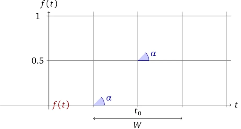
t f(t) f(t) α α t0 W 0.5 1

Figure 6.1: A sigmoid function f(t) =1/(1+e−s(t−t0))_.

6.1.2

ConceptDriftStream

Generator that adds concept drift to examples in a stream.

Considering data streams as data generated from pure distributions, MOA models a concept drift event as a weighted combination of two pure distribu-tions that characterizes the target concepts before and after the drift. MOA uses the sigmoid function, as an elegant and practical solution to define the probability that every new instance of the stream belongs to the new concept after the drift.

We see from Figure6.1that the sigmoid function f(t) =1/(1+e−s(t−t0))

has a derivative at the point t₀ equal to f0(t₀) =s/4. The tangent of angleα is equal to this derivative, tanα =s/4. We observe that tanα=1/W, and as s=4 tanα thens=4/W. So the parameters in the sigmoid gives the length of W and the angle α. In this sigmoid model we only need to specify two parameters : t0 the point of change, andW the length of change. Note that for any positive real numberβ

f(t0+β·W) =1−f(t0−β·W),

and that f(t₀+β·W)and f(t₀−β·W)are constant values that don’t depend on t₀ andW:

f(t₀+W/2) =1−f(t₀₋W/2) =1/(1+e−2)_≈88.08% f(t₀+W) =1−f(t₀−W) =1/(1+e−4)≈98.20% f(t₀+2W) =1−f(t₀₋2W) =1/(1+e−8)_≈99.97%

6.1. STREAMS

Definition 1. Given two data streams a, b, we define c = a⊕W

t0 b as the data

stream built joining the two data streams a and b, where t₀is the point of change, W is the length of change and

• Pr[c(t) =a(t)] =e−4(t−t0)/W/(₁+_e−4(t−t0)/W) • Pr[c(t) =b(t)] =1/(1+e−4(t−t0)/W)_. Example: ConceptDriftStream -s (generators.AgrawalGenerator -f 7) -d (generators.AgrawalGenerator -f 2) -w 1000000 -p 900000 Parameters: • -s : Stream

• -d : Concept drift Stream

• -p : Central position of concept drift change • -w : Width of concept drift change

6.1.3

ConceptDriftRealStream

Generator that adds concept drift to examples in a stream with different classes and attributes. Example: real datasets

Example:

ConceptDriftRealStream -s (ArffFileStream -f covtype.arff) \

-d (ConceptDriftRealStream -s (ArffFileStream -f PokerOrig.arff) \ -d (ArffFileStream -f elec.arff) -w 5000 -p 1000000 ) -w 5000 -p 581012

Parameters: • -s : Stream

• -d : Concept drift Stream

• -p : Central position of concept drift change • -w : Width of concept drift change

6.1.4

FilteredStream

A stream that is filtered.

Parameters:

• -s : Stream to filter

• -f : Filters to apply : AddNoiseFilter

6.1.5

AddNoiseFilter

Adds random noise to examples in a stream. Only to use with FilteredStream. Parameters:

• -r : Seed for random noise

• -a : The fraction of attribute values to disturb • -c : The fraction of class labels to disturb

6.2 Streams Generators

The classes available to generate streams are the following:

6.2.1

generators.AgrawalGenerator

Generates one of ten different pre-defined loan functions It was introduced by Agrawal et al. in

[A] R. Agrawal, T. Imielinski, and A. Swami. Database mining: A perfor-mance perspective. IEEE Trans. on Knowl. and Data Eng., 5(6):914–925, 1993.

It was a common source of data for early work on scaling up decision tree learners. The generator produces a stream containing nine attributes, six nu-meric and three categorical. Although not explicitly stated by the authors, a sensible conclusion is that these attributes describe hypothetical loan ap-plications. There are ten functions defined for generating binary class labels from the attributes. Presumably these determine whether the loan should be approved.

A public C source code is available. The built in functions are based on the paper (page 924), which turn out to be functions pred20 thru pred29 in the

6.2. STREAMS GENERATORS

public C implementation Perturbation function works like C implementation rather than description in paper

Parameters:

• -f : Classification function used, as defined in the original paper. • -i : Seed for random generation of instances.

• -p : The amount of peturbation (noise) introduced to numeric values • -b : Balance the number of instances of each class.

6.2.2

generators.HyperplaneGenerator

Generates a problem of predicting class of a rotating hyperplane. It was used as testbed for CVFDT versus VFDT in

[C] G. Hulten, L. Spencer, and P. Domingos. Mining time-changing data streams. In KDD’01, pages 97–106, San Francisco, CA, 2001. ACM Press.

A hyperplane in d-dimensional space is the set of points x that satisfy

d X i=1 w_ix_i=w₀= d X i=1 w_i

where x_i, is the ith coordinate of x. Examples for which Pd_i=1w_ix_i ≥ w₀ are labeled positive, and examples for whichPd_i=1w_ix_i <w₀ are labeled negative. Hyperplanes are useful for simulating time-changing concepts, because we can change the orientation and position of the hyperplane in a smooth manner by changing the relative size of the weights. We introduce change to this dataset adding drift to each weight attributew_i =w_i+dσ, whereσis the probability that the direction of change is reversed and d is the change applied to every example.

Parameters:

• -i : Seed for random generation of instances. • -c : The number of classes to generate • -a : The number of attributes to generate. • -k : The number of attributes with drift.

• -t : Magnitude of the change for every example • -n : Percentage of noise to add to the data.

• -s : Percentage of probability that the direction of change is reversed

6.2.3

generators.LEDGenerator

Generates a problem of predicting the digit displayed on a 7-segment LED display.

This data source originates from the CART book. An implementation in C was donated to the UCI machine learning repository by David Aha. The goal is to predict the digit displayed on a seven-segment LED display, where each attribute has a 10% chance of being inverted. It has an optimal Bayes classification rate of 74%. The particular configuration of the generator used for experiments (led) produces 24 binary attributes, 17 of which are irrelevant.

Parameters:

• -i : Seed for random generation of instances. • -n : Percentage of noise to add to the data

• -s : Reduce the data to only contain 7 relevant binary attributes

6.2.4

generators.LEDGeneratorDrift

Generates a problem of predicting the digit displayed on a 7-segment LED display with drift.

Parameters:

• -i : Seed for random generation of instances. • -n : Percentage of noise to add to the data

• -s : Reduce the data to only contain 7 relevant binary attributes • -d : Number of attributes with drift

6.2. STREAMS GENERATORS

6.2.5

generators.RandomRBFGenerator

Generates a random radial basis function stream.

This generator was devised to offer an alternate complex concept type that is not straightforward to approximate with a decision tree model. The RBF (Radial Basis Function) generator works as follows: A fixed number of ran-dom centroids are generated. Each center has a ranran-dom position, a single standard deviation, class label and weight. New examples are generated by selecting a center at random, taking weights into consideration so that centers with higher weight are more likely to be chosen. A random direction is chosen to offset the attribute values from the central point. The length of the displace-ment is randomly drawn from a Gaussian distribution with standard deviation determined by the chosen centroid. The chosen centroid also determines the class label of the example. This effectively creates a normally distributed hy-persphere of examples surrounding each central point with varying densities. Only numeric attributes are generated.

Parameters:

• -r : Seed for random generation of model • -i : Seed for random generation of instances • -c : The number of classes to generate • -a : The number of attributes to generate • -n : The number of centroids in the model

6.2.6

generators.RandomRBFGeneratorDrift

Generates a random radial basis function stream with drift. Drift is introduced by moving the centroids with constant speed.

Parameters:

• -r : Seed for random generation of model • -i : Seed for random generation of instances • -c : The number of classes to generate • -a : The number of attributes to generate • -n : The number of centroids in the model • -s : Speed of change of centroids in the model. • -k : The number of centroids with drift

6.2.7

generators.RandomTreeGenerator

Generates a stream based on a randomly generated tree.

This generator is based on that proposed in

[D] P. Domingos and G. Hulten. Mining high-speed data streams. In Knowl-edge Discovery and Data Mining, pages 71–80, 2000.

It produces concepts that in theory should favour decision tree learners. It constructs a decision tree by choosing attributes at random to split, and as-signing a random class label to each leaf. Once the tree is built, new examples are generated by assigning uniformly distributed random values to attributes which then determine the class label via the tree.

The generator has parameters to control the number of classes, attributes, nominal attribute labels, and the depth of the tree. For consistency between experiments, two random trees were generated and fixed as the base concepts for testingâ˘AˇTone simple and the other complex, where complexity refers to the number of attributes involved and the size of the tree.

A degree of noise can be introduced to the examples after generation. In the case of discrete attributes and the class label, a probability of noise param-eter dparam-etermines the chance that any particular value is switched to something other than the original value. For numeric attributes, a degree of random noise is added to all values, drawn from a random Gaussian distribution with stan-dard deviation equal to the stanstan-dard deviation of the original values multiplied by noise probability.

Parameters:

• -r: Seed for random generation of tree • -i: Seed for random generation of instances • -c: The number of classes to generate

• -o: The number of nominal attributes to generate • -u: The number of numeric attributes to generate

• -v: The number of values to generate per nominal attribute • -d: The maximum depth of the tree concept

• -l: The first level of the tree above maxTreeDepth that can have leaves • -f: The fraction of leaves per level from firstLeafLevel onwards

6.2. STREAMS GENERATORS

6.2.8

generators.SEAGenerator

Generates SEA concepts functions. This dataset contains abrupt concept drift, first introduced in paper:

[S] W. N. Street and Y. Kim. A streaming ensemble algorithm (SEA) for large-scale classification. In KDD ’01, pages 377–382, New York, NY, USA, 2001. ACM Press.

It is generated using three attributes, where only the two first attributes are relevant. All three attributes have values between 0 and 10. The points of the dataset are divided into 4 blocks with different concepts. In each block, the classification is done using f₁+f₂≤θ, where f₁ and f₂ represent the first two attributes andθ is a threshold value. The most frequent values are 9, 8, 7 and 9.5 for the data blocks.

Parameters:

• -f: Classification function used, as defined in the original paper • -i: Seed for random generation of instances

• -b: Balance the number of instances of each class • -n: Percentage of noise to add to the data

6.2.9

generators.STAGGERGenerator

Generates STAGGER Concept functions. They were introduced by Schlimmer and Granger in

[ST] J. C. Schlimmer and R. H. Granger. Incremental learning from noisy data. Machine Learning, 1(3):317–354, 1986.

The STAGGER Concepts are boolean functions of three attributes encoding objects: size (small, medium, and large), shape (circle, triangle, and rectan-gle), and colour (red,blue, and green). A concept description covering ei-ther green rectangles or red triangles is represented by (shape=rectangle and colour=green) or (shape=triangle and colour=red).

Parameters:

1. -i: Seed for random generation of instances

2. -f: Classification function used, as defined in the original paper 3. -b: Balance the number of instances of each class

6.2.10

generators.WaveformGenerator

Generates a problem of predicting one of three waveform types.

It shares its origins with LED, and was also donated by David Aha to the UCI repository. The goal of the task is to differentiate between three differ-ent classes of waveform, each of which is generated from a combination of two or three base waves. The optimal Bayes classification rate is known to be 86%. There are two versions of the problem, wave21 which has 21 nu-meric attributes, all of which include noise, and wave40 which introduces an additional 19 irrelevant attributes.

Parameters:

• -i: Seed for random generation of instances • -n: Adds noise, for a total of 40 attributes

6.2.11

generators.WaveformGeneratorDrift

Generates a problem of predicting one of three waveform types with drift. Parameters:

• -i: Seed for random generation of instances • -n: Adds noise, for a total of 40 attributes • -d: Number of attributes with drift

7

Classifiers

The classifiers implemented in MOA are the following:

• Bayesian classifiers – Naive Bayes

– Naive Bayes Multinomial • Decision trees classifiers

– Decision Stump – Hoeffding Tree

– Hoeffding Option Tree – Hoeffding Adaptive Tree • Meta classifiers

– Bagging – Boosting

– Bagging using

ADWIN

– Bagging using Adaptive-Size Hoeffding Trees. – Perceptron Stacking of Restricted Hoeffding Trees – Leveraging Bagging

• Function classifiers – Perceptron

– SGD: Stochastic Gradient Descent – Pegasos

• Drift classifiers

7.1 Bayesian Classifiers

7.1.1

NaiveBayes

Performs classic bayesian prediction while making naive assumption that all inputs are independent.

Naïve Bayes is a classifier algorithm known for its simplicity and low com-putational cost. Given n_C different classes, the trained Naïve Bayes classifier predicts for every unlabelled instance I the class C to which it belongs with high accuracy.

The model works as follows: Let x₁,. . . , x_k be k discrete attributes, and assume thatx_i can taken_i different values. LetC be the class attribute, which can taken_C different values. Upon receiving an unlabelled instance I = (x₁= v₁, . . . ,x_k=vk), the Naïve Bayes classifier computes a “probability” of I being in classc as: Pr[C =c_|I] ∼= k Y i=1 Pr[x_i =v_i|C =c] = Pr[C =c]· k Y i=1 Pr[x_i=v_i∧C =c] Pr[C =c]

The values Pr[x_i =v_j∧C =c]and Pr[C =c]are estimated from the train-ing data. Thus, the summary of the traintrain-ing data is simply a 3-dimensional table that stores for each triple (x_i,v_j,c) a count N_i,j,c of training instances

withx_i=v_j, together with a 1-dimensional table for the counts ofC =c. This algorithm is naturally incremental: upon receiving a new example (or a batch of new examples), simply increment the relevant counts. Predictions can be made at any time from the current counts.

Parameters:

• -r : Seed for random behaviour of the classifier

7.1.2

NaiveBayesMultinomial

Multinomial Naive Bayes classifier. Performs text classic bayesian prediction while making naive assumption that all inputs are independent. For more information see,

[MCN] Andrew Mccallum, Kamal Nigam. A Comparison of Event Models for Naive Bayes Text Classification. InAAAI-98 Workshop on ’Learning for Text Categorization’, 1998.

7.2. DECISION TREES

The core equation for this classifier:

P[C_i|D] = (P[D|C i]x P[C_i])/P[D](Bayes rule) where C_i is classiand Dis a document.

Parameters:

• -l : Laplace correction factor

7.2 Decision Trees

7.2.1

DecisionStump

Decision trees of one level.

Parameters:

• -g : The number of instances to observe between model changes • -b : Only allow binary splits

• -c : Split criterion to use. Example : InfoGainSplitCriterion • -r : Seed for random behaviour of the classifier

7.2.2

HoeffdingTree

Decision tree for streaming data.

A Hoeffding tree is an incremental, anytime decision tree induction algo-rithm that is capable of learning from massive data streams, assuming that the distribution generating examples does not change over time. Hoeffding trees exploit the fact that a small sample can often be enough to choose an optimal splitting attribute. This idea is supported mathematically by the Hoeffding bound, which quantifies the number of observations (in our case, examples) needed to estimate some statistics within a prescribed precision (in our case, the goodness of an attribute). More precisely, the Hoeffding bound states that with probability 1−δ, the true mean of a random variable of range R will not differ from the estimated mean afternindependent observations by more than:

ε=

r

R2_ln(1/δ) 2n .

A theoretically appealing feature of Hoeffding Trees not shared by other incre-mental decision tree learners is that it has sound guarantees of performance.