Autonomous Deployment for Load Balancing
k
-Surface Coverage in Sensor Networks
∗
Feng Li, Jun Luo, Wenping Wang, and Ying He
Abstract—Although the problem of k-area coverage has been intensively investigated for dense wireless sensor networks
(WSNs), how to arrive at a k-coverage sensor deployment
that optimizes certain objectives in relatively sparse WSNs still faces both theoretical and practical difficulties. Moreover, only a handful of centralized algorithms have been proposed to elevate 2D area coverage to 3D surface coverage. In this paper, we present a practical algorithm APOLLO (Autonomous dePlOyment for Load baLancing k-surface cOverage) to move sensor nodes toward k-surface coverage, aiming at minimizing the maximum sensing range required by the nodes. APOLLO enables purely autonomous node deployment as it only entails localized computations. We prove the termination of the algo-rithm, as well as the (local) optimality of the output. We also show that our optimization objective is closely related to other frequently considered objectives for 2D area coverage. Therefore, our practical algorithm design also contributes to the theoretical understanding of the 2D k-area coverage problem. Finally, we use extensive simulation results to both confirm our theoretical claims and demonstrate the efficacy of APOLLO.
Index Terms—Wireless sensor networks, autonomous deploy-ment, k-area/surface coverage, load balancing.
I. INTRODUCTION
One of the major functions of wireless sensor networks (WSNs) is to monitor a certain area in terms of whatever physical quantities demanded by applications [2]. In achieving this goal, a basic requirement imposed onto WSNs is their area/surface coverage:1 it indicates the monitoring quality of WSNs. Whereas many research proposals focus on either analyzing the performance of static sensor deployments (e.g., [5], [25]) or scheduling sensor activity to retain the coverage of given deployments (e.g., [33], [45]), there exists an unfailing trend in seeking autonomous deployments assisted by mobile sensor nodes to arrive at certain predefined objectives (e.g., [6], [34]). Our proposal in this paper falls into this later trend. Due to the vulnerability of sensor nodes, multiple-coverage (k-coverage) is often applied to enhance the fault tolerance The preliminary conference version of this paper has been published by IEEE ICDCS 2012 [28], where our focus was only on 2Dk-area coverage. In this paper, we generalize [28] to 3D k-surface coverage. This work is supported in part by AcRF Tier 2 Grant ARC15/11.
Feng Li, Jun Luo, and Ying He are with School of Computer Engi-neering, Nanyang Technological University, Singapore. E-mail:{fli3, junluo, yhe}@ntu.edu.sg
Wenping Wang is with Department of Computer Science, The University of Hong Kong, China. E-mail: [email protected]
1For WSNs deployed on 2D planes, we only focus on approaches
concern-ing area coverage (e.g., [5], [25]), as opposed to thepoint coverage(e.g., [8], [14], [44]). Surface coverage is an elevation of area coverage from 2D planes to 3D surfaces (terrains), making the deployment more useful in practice (e.g., for monitoring volcanos).
in face of node failures (e.g., [5], [45]). In addition, k -coverage may yield higher sensing accuracy through data fusion [13]. Existing approaches in achievingk-coverage rely on either randomized (e.g., [15], [25]) or regular (e.g., [3], [5]) deployments. Whereas randomized deployments require a substantially denser network (e.g., [15], [25]), regular deploy-ments serve only as theoretical guidelines [3], [5] as they often require centralized coordinations and may not accommodate irregular network regions. Also, if the physical phenomena under surveillance change, the cost for re-deployment can be huge. Therefore, autonomous deployments, when movable nodes [10] are available, are good complements to the ran-domized or regular deployments: they may achieve a density comparable to that of regular deployments, while being more adaptive to irregularity and variations of the network regions. However, existing techniques for autonomous deployments may only handle 1-coverage, and extending them to k -coverage is highly nontrivial. First of all, autonomous de-ployments through (node) motion control require each node to compute its coverage in a localized manner (i.e., relying as much as possible on close-by nodes). Although quite a few localized algorithms have been proposed to perform such computations for 1-coverage (e.g., [7], [34]), no algorithm, to the best of our knowledge, exists for localized k-coverage computations. Secondly, even if thek-coverage computations can be performed locally, there is no guarantee whether a motion control strategy may converge, due to the significant difference between 1-coverage and k-coverage. Thirdly, ex-isting approaches are almost heuristics that offer no provable guarantee on the quality of the eventual deployment. Finally, as indicated in [43], extending 2D area coverage to 3D surface coverage for WSNs deployed on 3D terrains may incur new challenges even for 1-coverage. By far, only a handful of proposals employ (partially) centralized algorithms to handle the deployment for 1-surface coverage [18], [43]; no pure autonomous deployment mechanism has ever been proposed. These are exactly the problems we want to tackle in our paper. In this paper, we consider the problem of moving sensor nodes towards k-coverage. In particular, we assume that n-odes have tunable sensing ranges and are randomly deployed initially. Our goal is to cover a certain monitored area or surface to the extent that every point in this area/surface is at least monitored by k sensor nodes and that the maximum sensing range used by the nodes is minimized. As a larger sensing range implies a larger energy consumption of a node, our APOLLO (Autonomous dePlOyment for Load baLancing
k-surface cOverage) approach aims at balancing the sensing load (thus prolonging network lifetime) while guaranteeing
k-coverage, with the help of mobile nodes. The main contri-butions we are making in this paper are:
• We design the APOLLO algorithm such that it executes in a localized manner, i.e., relying only on information from close-by nodes.
• We prove the termination of APOLLO as well as the (local) optimality of its output.
• We discuss the relation between APOLLO and other com-monly used optimization objectives for 2D area coverage, which provides a better understanding of optimal k -coverage deployments whose theoretical characterizations are hard to obtain under general settings.
• We show that, by using geodesic distance [9] to replace the conventional Euclidean metric, APOLLO can be naturally extended to handle autonomous deployments on 3D surfaces.
• Since motion and communication cost cannot be neglect-ed, our algorithm allows for a tradeoff between the two factors. Through extensive simulations driven by realistic power consumption data, we show that the existing hard-ware platform can afford the energy consumption of our algorithm in terms of motion and communication. To the best of our knowledge, we are the first to tackle the problem of k-coverage autonomous deployment, for both 2D areas and 3D surfaces.
The remaining of our paper is organized as follows. We briefly survey the closely related literature in Sec. II. We formally define our model and problem in Sec. III, in which we also review the basic mathematical tools we need in our later algorithm design. In Sec. IV, we present our APOLLO algorithm for 2Dk-area coverage and analyze its performance, we also interpret our solution with respect to other optimiza-tion frameworks. We then extend APOLLO to handle 3D k -surface coverage in Sec. V. The efficacy of APOLLO is further confirmed by extensive simulation results reported in Sec. VI. We finally conclude our paper in Sec. VII.
II. RELATEDWORK
Before surveying the proposals related to area/surface cov-erage and mobile assisted autonomous deployment, we first review another interesting topics, point (or target) coverage and area coverage with random deployments, from which we may gain some hints for our proposal. Point coverage problem has been extensively studied in the past decade. Besides providing coverage service, their another concern is the limited energy supply of sensor nodes. Given a random deployment with static sensor nodes, they either divide the nodes into multiple sets and schedule the duties of these set (e.g. [8], [11], [44]), or minimize the number of the active sensor nodes (e.g., [14]), to guarantee the network lifetime. The energy limitation is also taken into account in area coverage with random deployments, e.g. [21], [25], [38], [41], [45]. Inspired by them, maximizing the network lifetime is also one of the main objectives of our proposal but in a quite different way.
The static and deterministic area coverage problem is es-sentially a geometry problem; the results for 1-coverage with a minimum number of nodes can be directly taken from
pure mathematical research [22]. In later research proposals for WSN coverage, the focus is more on minimum node 1-coverage with certain connectivity requirement (e.g., [4], [5], [19]). While it is known that a 1-covered WSN is also connected if the transmission rangeRt and the sensing range Rs satisfy Rt≥
√
3Rs, a strip-based deployment strategy is
proposed in [19] for other values of Rt, which is proven to
be asymptotically optimal in [4]. In fact, more strips allows higher degree of connectivity (ork-connectivity).
Compared with k-connectivity, the progress on k-coverage appears to be relatively slower. A few 3-coverage heuristics that aim at bounding the minimum separation among sensor nodes is proposed in [23]; the paper also shows that bounding the min-separation may lead to lower coverage redundancy and is hence a good approximation to minimum node3-coverage. To the best of our knowledge, the only optimality result in terms of minimum nodek-coverage is presented in [5], where
k= 2. It appears that minimum nodek-coverage (for k >2) is better to be tackled indirectly due to its hardness. As we will show in Sec. IV-C, our objective of a k-coverage with mini-max sensing range may also imply minimum nodek-coverage. Deploying WSNs for k-coverage using mobile nodes is also reported in [3], [36], but their approaches are not autonomous as they all rely on a “blueprint” to guide the node mobility.
Considering that a WSN can be deployed on a 3D terrain for some application scenario, the surface coverage problem has also been investigated. Zhao et al. [24], [43] show that extending just 1-area coverage to 1-surface coverage already poses great challenges, and they provide approximation algo-rithms to the resulting NP-complete problem. Recently, Jinet al. [18] applies Centroid Voronoi Tessellation (CVT) [12] and discrete Ricci flow [17] to obtain some form of optimal surface 1-coverage by defining sensing range upon geodesic distance. However, the discrete Ricci flow is a global parametrization process, so the motion control cannot be implemented in a distributed manner using only local information.
Our work is also related to the sensing heterogeneity issue [6], [35]. Unlike the previous proposals that aim to cope with sensing heterogeneity or evaluate its impact, we actively exploit the sensing heterogeneity to construct our algorithm that guides the autonomous deployment.
III. PROBLEMDEFINITION ANDMATHEMATICAL BACKGROUND
In this section, we first present the system model and define our optimization problem, and then introduce the relevant mathematical basics. To simplify the exposition, the above discussions are all for 2D plane with Euclidean metric. We then show that a 2D plane can be straightforwardly generalized to a 3D surface by replacing Euclidean metric with geodesic distance, and we also introduce the mathematical tools to perform this map locally.
A. System Model
We assume a WSN consisting of a setN ={n1,· · ·, nN}
of sensor nodes, and|N |=N. LetU ={u1,· · · , uN}denote
the locations of sensor nodes. The nodes are initially deployed arbitrarily on a 2Dtargeted areaA. Each nodeniis equipped
with certain mechanisms (e.g., motors plus wheels) that allow it to gradually change its location ui [10]. We also suppose
that nodes are equipped with bumper sensors to detect and avoid obstacles in the targeted area [30]. All nodes have an identical transmission range γ, and we denote by N(ni) =
{nj|∥ui−uj∥2≤γ, i̸=j} the one-hop neighbors ofni.
We define the omnidirectional sensing model as a disk centered at ui with sensing range ri. We assume the
sens-ing ranges are adjustable accordsens-ing to different application requirements [42], [45]. A pointv∈ Ais said to be covered by nodeniiff the Euclidean distance betweenvand node location uiis no longer thanri, i.e.,∥v−ui∥2≤ri. We usef(v, ui, ri)
to indicate if v is covered by node ni: f(v, ui, ri) = 1 if v
is covered by ni; otherwise, f(v, ui, ri) = 0. We apply the
MDS-based technique [30] that relies on the ranging ability of each node to construct a local coordinate system for motion control, but we do not require global location information as it is immaterial to our algorithm.
In terms of energy cost, we consider only the cost induced by the sensing activities of a node. Because our network de-ployment strategy aims to achieve a constant (and long-term) coverage by moving sensor nodes in the initial phase, the com-munication cost becomes negligible as the data transmission activities only take place sporadically, while the energy spent in moving is only a one-time investment. We assume that the energy consumed by a sensor nodeniis an increasing function E(ri)of its sensing rangeri, and this function is identical for
all nodes. In other words, with a certain amount of energy
E(ri),ni can only cover the points{v∈ A|∥v−ui∥2≤ri}.
B. Problem Formulation
The node locations and sensing ranges define a network deployment with a certain coverage.
Definition 1. A network deployment{ui, ri}is said to achieve k-coverage iff for any pointv∈ A, there existat leastksensor nodes covering it, or ∑if(v, ui, ri)≥k.
To allow the sensor nodes k-cover the targeted area, we divideAinto several disjoint areas{Akj}j=1,2,..., and at least ksensor nodes are allocated to take care of each area. In other words, each sensor node ni takes care of multiple subareas,
and we indicate this covering relation by ni(Akj): it equals 1
ifni coversAkj; otherwise 0. We also denote byAkni the area
covered by ni: we have Akni =
∪
ni(Akj)=1A
k
j. The sensing
rangeriofni is determined by the farthest point inAkni from ui, i.e.,ri= maxv∈Ak
ni∥v−ui∥2, so thatA k
ni can be totally
covered by ni.
Our k-coverage sensor deployment problem(k-CSDP) can be formulated as follows. minimize {ui},{Ak j},{ni(Akj)} R (1) subject to ∑Ni=1f(v, ui, ri)≥k, ∀v∈ A (2) ∥v−ui∥2≤R, ∀i, v∈ Akni (3) Ak j1 ∩ Ak j2 =∅, ∪ jAkj =A (4)
Literally, k-CSDP aims at determining the node locations
{ui}, the area partition {Akj}, and the covering relations
{
ni(Akj)
}
, such that the targeted area Ais k-covered, while the maximum sensing range among all nodes is minimized. As energy consumption is an increasing function of sensing range,
k-CSDP is equivalently balancing the energy consumption over a whole WSN and hence maximizing the lifetime of the WSN. As the problem is generally not convex due to its non-convex feasible region, we have to be contented with local minimum(i.e., a locally minimized maximum sensing range). C. High Order Voronoi Diagram
We hereby briefly introduce the ideas and theories onhigh order Voronoi diagram[31]. They are key to our autonomous deployment strategy.
In a k-order Voronoi diagram, the targeted area A is segmented into Nˆk disjoint areas {Vk
j}j=1,...,Nˆk,2 each of
which is associated with k closest generators (sensor nodes in our case), i.e., a subset Nk
j ⊆ N with |Njk| = k. The k-order Voronoi cell Vjk is defined as
Vk j = { v∈ A ∀∥v−ui∥2 ≤ ∥v−ui′∥2, ni ∈ Njk, ni′∈ N/Njk } (5) The set Nk
j is called the generator set of Vjk. It is
straight-forward to see that each sensor node ni is associated with
multiple Voronoi cells. LetVnkidenote the union of the Voronoi
cells for which ni serves as a generator; we term Vnki the
dominating regionofni (hencenithedominatorof Vnki). We
also have the following proposition.
Proposition 1. A pointv∈ Ais said to belong toVnkiiff there
exist at mostk−1 other generators such that their distance tov is less than∥v−ui∥2.
Proof: Assume v∈ Vnik but there were another k nodes
{nj}j∈J,i̸∈J,|J|=k such that∥uj−v∥2<∥ui−v∥2. Then the
point v would strictly belong to the set of k-order Voronoi cells generated by {nj}, which does not include ni as a
generator; a contradiction. Conversely, if there are at most
k−1 nodes, {nj}j∈J,i̸∈J,|J|≤k−1, closer to v than ni, we
can find the set of v’s k-nearest nodes (which obviously contains {nj}
∪
{ni}) to generate a set of k-order Voronoi
cells containingv. Asni is a generator,v∈ Vnki.
Based on the above proposition, assumingSnki(v) ={nj ∈
N |∥uj −v∥2 < ∥ui −v∥2, j ̸= i}, we can re-define the
dominating region ofni as
Vk
ni ={v∈ A | |S k
ni(v)| ≤k−1} (6)
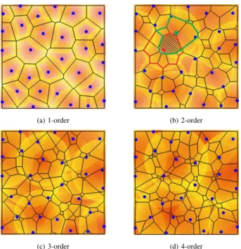
We illustratek-order Voronoi partition (k = 1,2,3,4) gener-ated by 30 nodes in Fig. 1. The cells shown in each figure are
{Vk
j}. Taking2-order Voronoi partition for example, as shown
in Fig. 1(b), the area enclosed by red (resp. green) polygon is actually the dominating region of the red node (resp. green node). The hatched area is the Voronoi cell generated by the two nodes, i.e., the points in this area are closer to the two nodes than any other nodes.
2In1-order Voronoi diagram, the number of Voronoi cells equals the number
of generators (i.e.,Nˆ1=N), while in generalizedk-order Voronoi diagram (k≥1),NˆkisO(k(N−k))[31].
(a) 1-order (b) 2-order
(c) 3-order (d) 4-order
Fig. 1. k-order Voronoi partition fork= 1,2,3,4. The disks at the backdrop represent the (overlapping) sensing ranges of individual sensor nodes. D. Generalization to 3D Surfaces
For WSN deployed on a 3D surface, the conventional Euclidean metric is no longer appropriate. Serving as the generalization of “straight line” in curved space (e.g., 3D surfaces), geodesic is the shortest path between two given points on the surface [9]. Therefore, geodesic distance metric is a natural choice for measuring distance on a 3D surface. By replacing Euclidean metric with geodetic distance, we may migrate the aforementioned model and problem definitions directly from 2D planes to 3D surfaces.
1) Problem Description on 3D Surfaces: Consider the case where a WSN N is deployed on the 3D surface M, we use geodesic distance as the distance metric. In particular, we replace all the distant metric∥u−v∥2 used for 2D planes by
g(u, v), the geodesic distance betweenuandv. As a result, all
the definitions in Sec. III-A to III-C can be directly migrated to 3D surface. For example, k-CSDP and high order Voronoi diagram can be redefined using geodesic metric. The only difference here is that, while A does not need an explicit characterization,Mis often represented by a triangular mesh that is given to all nodes during the initialization phase.
In order to compute geodesic distance on M, we adopt the Improved Chen & Han’s (ICH) algorithm [39]. The ICH algorithm handles the “single source, all destinations” geodesic problem, aiming at computing the geodesic from the source
u ∈ M to any destination point v ∈ M within a certain geodesic radius rfrom near to far with a time complexity of
O(n2logn)wherenis the number of vertices of the triangular
mesh M within r. It maintains a priority queue of geodesic windows on the edges of the triangular mesh, and outputs a poly-line geodesic path for each pair of source and destination. The ICH algorithm also can be extended to other types of geodesic problem [40], e.g., “single source, single destination” and “multiple sources, any destination”. Such a package of geodesic computation tools is sufficient for our 3D extension.
2) Logarithm and Exponential Maps: As we need a local coordinate system to compute k-order Voronoi diagrams in a localized manner for every node, we cannot rely on a parametrization method such as Ricci flow due to its global nature and high computational cost. We instead apply the ICH algorithm to compute an logarithm/exponential map [9] around a certain node, which constructs a (local) geodesic polar coordinate system on the curved surface as follows.
Given a point u ∈ M, we designate a local coordinate system on its tangent planeTucentered atu. Alogarithm map
exp−1
u :M → Tumaps the points on MtoTu. In particular,
for any other pointv∈ Min a sufficiently small neighborhood of u, there is a unique geodesic Gu(v) extending fromu to
v. As G′u(v), the tangent of Gu(v), is obviously tangent to
Matu,G′u(v)∈ Tu. Therefore,v can be mapped toTu with
geodesic polar coordinates{g(u, v), θu,v}whereg(u, v)is the
geodesic distance betweenuandvandθu,v is the polar angle
of G′u(v) on Tu. Consequently, the geodesic coordinates on
Marounducan be transformed to normal coordinates under any orthogonal basis {e1,e2} with origin u. The inverse of
logarithm map is called exponential map. We illustrate the log/exp map in Fig. 2. Here the ICH algorithm [39] is used
(a) Coordinate system inTu (b) Coordinate system inM Fig. 2. The log/exp maps at pointuintroduces a mapping between a vector originating atuonTuand a geodesic beginning atuonM. The circles on
Tuare mapped to the contours of the geodesic function onM.
to trace the geodesic Gu(v) such that any point v in the neighborhood ofuonMcan get its geodesic polar coordinates on Tu. As mentioned above, the ICH algorithm maintains a
“wavefront” and propagates outward fromu, finally outputting a local geodesic coordinate system within a radiusr.
IV. APOLLO: LOCALIZEDk-COVERAGENODE DEPLOYMENTALGORITHM
In this section, we first develop two optimality conditions fork-CSDP. Then we present the APOLLO algorithm details. The correctness of APOLLO is then proven, and we finally discuss the relation betweenk-CSDP and other optimization problems related to k-coverage deployment, along with the corresponding properties of APOLLO.
A. Optimal Conditions
To motivate our algorithm, we develop two optimality conditions fork-CSDP. Firstly, we show if we fix{ui}, then k-order Voronoi diagram is the optimal solution tok-CSDP.
Proposition 2. If we fix the sensor locations {ui}, the k
partition of A. Also, ni(Vjk) = 1 if Vjk ⊆ Vnki; otherwise ni(Vjk) = 0.
Proof: The proof is by contradiction. Suppose for fixed
{ui}i=1,···,N, there exists an optimal solution tok-CSDP
de-noted byR∗,{A¯kj},{ni( ¯Akj) } . Letr∗i = maxv∈A¯k ni∥v−ui∥2 andrV i = maxv∈Vk
ni∥v−ui∥2. Also assume that the optimal
value is obtained for nˆi, i.e., R∗ = rˆi∗. If rˆVi = rˆi∗, then it
is straightforward to see that rV
ˆi = maxi{r
V
i }, otherwise a
contradiction to the definition of Vnki: some regions are not
covered by the k-closest nodes. Therefore, in this case the
k-order Voronoi diagram is equally optimal. If rˆiV > rˆ∗i, it means that nˆi could cede a certain region to have it covered
by other nodes while reducingmaxi{rVi }. However, this again
contradicts the definition of Vk
ni: as nˆi is already one of the k-closest nodes that can cover the ceded region, ceding this region to some other nodes would increase maxi{rVi }.
Before stating the second optimality condition, we need the following definition.
Definition 2. Given an arbitrary set S in Euclidean s-pace, the Chebyshev center uc is defined as uc = arg minuˆ(maxu∈S∥u−ˆu∥2)
Given an area partition {Ak
j} and its dominator allocation
(or covering relations) {ni(Akj)
}
, the optimal locations of
{ni}can be obtained according to the following proposition.
Proposition 3. If we fix the partition{Ak
j}and its dominator
allocation {ni(Akj)
}
, the optimal sensor location u∗i for k -CSDP is given by the Chebyshev center of Ak
ni.
Proof: Asni needs to cover Akni and the objective of k
-CSDP is to minimize the maximum sensing range among all sensors, the optimal solution under a fixed partition is achieved if each sensor individually minimizes its own sensing range. This exactly coincides with the property of Chebyshev center, hence the proposition follows.
B. The Algorithm
Given the two optimality conditions stated in Sec. IV-A, we immediately have an iterative algorithm to solvek-CSDP. The pseudo-codes of our APOLLO algorithm are presented in Algorithm 1. The algorithm proceeds in rounds. At the
Algorithm 1: APOLLO
Input: For eachni∈ N, initial locationu
(0)
i , stopping
toleranceε
Output:{u∗i} and{r∗i}
1 For every nodeni∈ N periodically (every τ ms):
2 Compute its dominating regionVnk
i
3 Compute the Chebyshev center ci ofVnki
4 if ∥ui−ci∥2> ϵthen
5 u+i ←ui+α(ci−ui) /*αis the step size*/
6 end
7 u∗i ←ci, ri∗←maxu∈Vk
ni∥u−ui∥2
beginning of each round, thek-order Voronoi diagram is com-puted for the whole WSN, resulting in{Vk
1,· · ·,VNkˆk} along
with{Vnk1,· · ·,V
k
nN}(Line 2). Then each node computes the
Chebyshev center of its dominating region (Line 3), and moves to that location to end this round (Line 4-6). The algorithm terminates if each node is indeed located at the Chebyshev center of its dominating region. As a perfect matching is impossible in face of numerical errors, we use a small value
ε as the stopping tolerance: the algorithm terminates if the distance from the node’s current location to the Chebyshev center of its dominating region is smaller thanε. Also, in order to avoid oscillation, a step sizeα <1is chosen to confine the motion of the nodes. At the termination, each node tunes its sensing range to be the minimum value (the circumradius of its dominating region) that covers its dominating region. As a dominating region is a polygon, we apply Welzl’s algorithm [37] to compute the Chebysehev center by taking the vertices of the region as the input.
Similar algorithms have been applied in [6], [34], but they were used to indirectly optimize a different objective (see our discussions in Sec. IV-C). Consequently, their approaches do not abide by the optimality conditions and employ a very different termination condition. Therefore, their termination proofs do not apply to our case even for k = 1. Most importantly, as our algorithm deals with a more general k -coverage, we are facing the following new challenges in understanding our algorithm: 1) How to compute Vk
ni in a
localized manner without involving all nodes? 2) Does the algorithm terminate fork≥1? 3) What is the complexity of computations? We tackle these challenges in the following.
1) Localized Algorithm for ComputingVk
ni: Unlike 1-order
Voronoi diagram that can be computed (mostly) by only interacting with one-hop neighborsN(ni)of a given nodeni,
N(ni) may not be sufficient to obtaink-order Voronoi cells,
especially whenkis large. The reason is simple: at leastk+ 1
nodes should be involved to compute a dominating region ofni
[26]. Therefore, we proposeAlgorithm 2 to locally calculate
Vk
ni in an expanding ring manner.
Algorithm 2: LocalizedVk
ni Computation
Input: For eachni∈ N, initial ring radiusρ= 0
Output: Vnki
1 repeat
2 ρ←ρ+γ; out←true 3 N(ni, ρ)← {nj|∥uj−ui∥2< ρ}
4 Construct a local coordinate system usingN(ni, ρ)
5 foreach v∈ As.t. ∥v−ni∥2=ρ/2 do
6 Sˆnik (v)← {nj∈ N(ni, ρ)|∥uj−v∥2< ∥ui−v∥2, j̸=i}
7 if|Sˆnk
i(v)|< kthen out←false; break
8 end
9 untilout=true; 10 ComputeVnk
i based on N(ni, ρ)
Basically, we expand the search ring ρ with a granularity of the transmission rangeγ (line 2). As expending ρbeyond
γ will need multi-hop communication and the hop number is always an integer, it makes no sense to apply a smaller granularity. We use the embedding algorithm proposed in [32] to construct a local coordinate system (line 4). If the location
information is available, this step is not necessary. Under the constructed coordinate system, we check whether the circle centered at ui with a radius ρ/2 is not dominated by ni
anymore (lines 5 to 8, based on Proposition 1). Because the Voronoi edges computed givenN(ni, ρ)divide the circle with
radiusρ/2 into a finite number of arcs, each of which either fully dominated by ni or not at all, we only need to check
an arbitrary point on each arc in the actual implementation. The ring expending terminates if the answer becomes true. Finally, we compute Vnki using only nodes falling into the
current search ring (line 10).
We need another lemma to show that Vnki computed by
Algorithm 2 is indeed the one that would be computed in a centralized manner using global information.
Lemma 1. If the dominating region of ni is enclosed by a
circle centered at ui with a radius of ρ/2, then it is fully
determined by all the nodes located within another circle centered atui with a radius ofρ.
Proof: For a disk ⊙(ui, ρ/2) centered at ui with radius ρ/2, if Vk
ni ⊂ ⊙(ui, ρ/2), the boundary of V
k
ni also belongs
to ⊙(ui, ρ/2). According to the definition of Voronoi cells,
the cell boundary consists of bisectors, each of which is determined by two generators. For Vk
ni, one generator isni,
and all other generators can be obtained by going through each segment (or bisectors) on the boundary ofVk
ni and identifying
another generator that determines this bisector along with
ni. Since the boundary of Vnik belongs to ⊙(ui, ρ/2), all
generators of Vnki belong to⊙(ui, ρ).
r r/2
Fig. 3. Recognizing the network boundary (the green dashed curve), a boundary node (dark) determines a searching ring (the outer circle) and check the half-radius arc within the network coverage area (the inner red arc). It then calculates its dominating region (the blue area) with N(ni, ρ), while the searching ring helps to determine part of the boundary.
The correctness of our algorithm is immediate from this lemma: as the algorithm terminates whenniis not dominating
the circle centered atuiwith a radiusρ/2anymore, the nodes
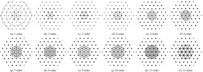
falling into ⊙(ui, ρ)are sufficient to computeVnki. In Fig. 4,
we demonstrate this sufficiency using k-order dominating region (k= 1to 12) in a regularly deployed WSN. The regular deployment is chosen to facilitate exposition, our algorithm works for any arbitrary deployments.
For a node ni on the boundary, the search ring will never
stop expanding, as the arc that is out of the network coverage will always need the domination ofni. To cope with this issue,
we first refer to our previous work [29] for an on-line boundary detection service. Sine each sensor node can identify if it is on the network boundary only relying on local positions of it one-hop neighbors, this boundary detection is highly efficient and
thus is quite suitable for our autonomous deployment. Based on the boundary awareness, the boundary node executes the circle checking procedure (lines 5 to 8) only for the arc that lies within the network coverage area, as shown in Fig. 3. Finally, the boundary node calculates its dominating region, using N(ni, ρ) as well as the searching ring to determine
the boundary of the dominating region. For an initial random deployment in which nodes only occupy a small fraction of
A, this procedure has the effect of “pushing” boundary nodes outwards, hence expanding the network coverage to the whole
A. In fact, such a constrained checking procedure should always be used by nodes on the boundary ofA, the difference is that A’s boundary, known in advance to the nodes, serves as a natural boundary for a dominating region.
2) Termination Analysis: Showing the termination of Al-gorithm 1 appears to be highly non-trivial, as many k -order Voronoi cells are concerning a certain node, and the dominating region of a node is mostly probably a non-convex region. Fortunately, the termination can be shown by focusing on the boundary of a dominating region.
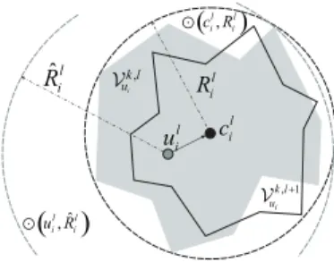
Proposition 4. Algorithm 1terminates forα∈(0,1]. Proof: As shown in Fig. 5, ul
i andVnik,l are the location
and dominating region of node ni at the beginning of the l-th round, respectively. We also denote by cli and Rli the Chebyshev center and the circumradius of Vnik,l computed
l i u cil , i l uk V , 1 i uk l+ V ˆl i R l i R
( )
u Rli, ˆil e ( , l) i l i c R eFig. 5. Notations in the proof for Proposition 4.
by ni during the l-round. Let Rˆil = maxu∈Vnik,l∥u−u l
i∥2
be the farthest distance from ul
i in Vnk,li. Finally, we define Rl= maxi{Rli}andRˆ
l= max
i{Rˆli}.
We first prove the termination forα= 1by contradiction. For eachni, we put a disk⊙(cli, Rl)centered atcliwith radius Rl. Obviously, ∪Ni=1⊙(cli, Rl) form a k-coverage over the targeted area A. The termination is naturally justified if we can prove that Vnk,li+1 is inside ⊙(c
l i, Rl) after uli is updated to cl i (i.e., u l+1 i = c l
i). For each point q on the boundary of
Vk,l+1
ni , it is straightforward to see thatc l
i is the location of the k-th nearest nodes. Assume thatq is outside⊙(cl
i, Rl), there
would be only k−1 disks coveringq, which contradicts the fact that∪Ni=1⊙(cl
i, Rl)constitute ak-coverage overA.
We then prove the termination for 0 < α < 1. Ac-cording to line 5 of Algorithm 1, during the l-th round,
uli+1=ul
i+α(cli−uli). We put disks⊙(uli,Rˆl)and⊙(cli,Rˆl)
centered at ul
i and cli, respectively. Obviously, Vnk,li is inside
⊙(uli,Rˆl)∩⊙(cil,Rˆl), which implies Vnk,li ⊂ ⊙(u
l+1
i ,Rˆ
l).
(a) 1-order (b) 2-order (c) 3-order (d) 4-order (e) 5-order (f) 6-order
(g) 7-order (h) 8-order (i) 9-order (j) 10-order (k) 11-order (l) 12-order Fig. 4. The dominating region of the central node ink-order Voronoi diagramk= 1,· · ·,12. The central node needs to collect location (or range) information from its neighboring nodes (the dark nodes) via multi-hop communication according toAlgorithm 2. Additionally, we illustrate multi-hop transmission range using red circles in (a). While the cases fork= 1can be handled by involving only the 6 closest nodes (1-hop neighbors) to the central node, computing the 2-, 3- and 4-order dominating regions requires 2-hop neighbors. Whenk >4, all sensor nodes within 3 hops are involved.
Following a similar argument as for α= 1, we have Vk,l+1
ni
is involved in ⊙(uli+1,Rˆl), which completes the proof.
In summary, our APOLLO algorithm terminates for any
α ∈ (0,1]. Usually, smaller α leads to slower convergence but smoother moving locus. As a byproduct of the proof, we also conclude that Rˆ is non-increasing iteratively and finally equivalent to R. Especially, when α = 1, R is also non-increasing in the iterative process. Therefore,
Corollary 1. Algorithm 1 terminates at a local minimum of
k-CSDP.
It is important to note that Rl andRˆl are introduced only
for our proof. During the algorithm execution, each node ni
can only compute its ownRl
iandRˆli. According to our earlier
discussion in Sec. IV-B1 (see Fig. 3 also), the evolution of the node positions often takes two phases: anexpandingphase and a convergingphase. The expanding phase exists if the initial node distribution is non-uniform, our APOLLO algorithm will force the node to spread out during this phase, as discussed at the end of Sec. IV-B1. During this phase, both RlandRˆl are most probably achieved by boundary nodes. The expanding phase ends when all the boundary nodes are at the boundary of A, this is when the converging phase starts.
3) Computational Complexity Analysis: Each iteration of APOLLO consists of two major steps: computing dominating regions and Chebyshev centers. The dominating regions are calculated in an expanding ring manner (seeAlgorithm 2). We supposeNi(ρ) =|N(ni, ρ)|is the number of the neighboring
nodes of ni within the searching ringρ. According to [26],
each sensor node computes local k-order Voronoi edges (as well as vertices) with a complexity ofO(k2N
i(ρ) logNi(ρ)).
Recall that Ni(ρ) leads to O(k(Ni(ρ)−k)) Voronoi edges
[31], the following checking operation has a complexity of
O(kNi(ρ)(Ni(ρ) −k)) in the worst case. The underlying
boundary detection service requires only one-hop neighbors, thus merely results in a negligible cost ofO(Ni(γ) logNi(γ))
[29]. Assuming up to H-hop neighbors are required (i.e.,
ρ expands from γ to Hγ with a granularity of γ), Algo-rithm 2 has a complexity of O(k2HN
i(Hγ) logNi(Hγ) +
kHNi(Hγ)(Ni(Hγ)−k)). For certain coverage orderk, the
overall complexity of Algorithm 2 is highly limited by the number of required communication hopsH. According to our experiments shown in Fig. 4, even the transmission range is restricted (only available for computing 1-order Voronoi domi-nating region), nodes within two or three hops are sufficient in most cases. Finally, givenO(k(Ni(Hγ)−k))Voronoi vertices
outputted byAlgorithm 2, we spend O(k(Ni(Hγ)−k)) on
computing their Chebyshev center [37].
The total number of iterations of APOLLO depends on individual cases, and thus cannot be derived by exiting analysis techniques. Similar with [6], [18], we will employ extensive simulations to reveal APOLLO’s convergence rate as well as the induced time cost in Sec. VI.
C. Discussions
In this section, we show the relations between the output of our APOLLO algorithm and other optimization objectives often considered for area coverage problems in WSNs.
Min-Node k-Coverage: One type of problem that is commonly tackled in the research community is to achieve
k-coverage using a minimum number of nodes (e.g., [3], [5], [43]). As this problem often assumes that all nodes have a fixed and identical sensing rangers, it appears that APOLLO
may not suggest a direct solution to it. However, we can transform our algorithm to deliver a good approximation to this min-node k-coverage problem as follows. APOLLO is called iteratively3 andR∗ is compared withr
s at the end of
each iteration. Nodes are added (resp. reduced) if R∗ > rs
(resp. R∗ < rs), until R∗ ≤ rs but adding one more node
would make R∗ > rs. Although the solution may not be
optimal, it yields very good approximation to the optimal solution, as we will demonstrate in Sec. VI. If fact, as the
3If an application only requires a one-time (rather than autonomous)
up-to-date algorithms are all approximations for k > 2 and they are not autonomous (e.g., [3]), our algorithm is also the first autonomous deployment for approximating min-node k -coverage with an arbitrary k.
Maximumk-Coverage: Another type of problem aims at maximizing coverage under fixed sensing ranges, but existing proposals only focus on 1-coverage [6], [18], [34]. A natural definition of the general maximum k coverage problem is to maximize the area that is k-covered under a fixed sensing range. The major difference between k = 1 and k > 1
is that the former achieves maximum coverage if nodes are far apart from each other whereas the same principle does not apply to the latter. An obvious example is the following: assume only 3 nodes are used to 3-cover an area, the maximum coverage is achieved only if all three nodes are put at the same location. Consequently, the heuristic of bounding the minimum separation among nodes [23] fails. Intuitively, APOLLO may deliver a good approximation to the maximum k-coverage problem, e.g., APOLLO terminates at the optimal solution for the aforementioned 3-node case.
Connectivity: Although maintaining network connectivi-ty is not our concern in designing APOLLO, it appears to be a natural outcome of achievingk-coverage fork≥2. Underk -coverage, it is easy to see that there should be at leastknodes in the sensing range ri of a nodeni (includingni), otherwise ui is not k-covered. In reality, as shown in Fig. 4, there are
at least 7 nodes in a certain sensing range for k≥2. Given the common assumption in the literature thatγ≥ri(e.g., [6],
[34], [44]), each node in a WSN has at least a degree of 6, which is sufficient to guarantee connectivity in the WSN.
Min-Max Fair: While ourk-CSDP only requires that the maximum sensing range is minimized and hence does not concern nodes with non-maximum sensing ranges, the min-max fair utility (a Pareto optimal point) requires that a nodeni
cannot further reduce its sensing rangesri without increasing
the sensing rangerj (rj ≥ri) of another nodenj. According
to the property of k-order Voronoi diagram, the output of APOLLO is at least locally optimal with respect to the min-max fair utility, i.e., if we reduce ri, another node nj that
shares dominating region boundary with ni should increase rj to maintain k-coverage, but we know rj ≥ ri before ri
gets reduced. In fact, our simulation results in Sec. VI show that, after APOLLO terminates, the maximum and minimum sensing ranges are almost the same fork >2.
V. APOLLOON3D SURFACES
Though replacing Euclidean metric by geodesic distance yields a straightforward extension of our problem from 2D planes to 3D surfaces (as we discussed in Sec. III-D), our APOLLO algorithm has to be slightly tuned to adapt to the local coordinate maps (i.e., the log/exp maps). As APOLLO (Algorithm 1) involves two main computations: dominating region and Chebyshev center, we present the APOLLO 3D extension with respect to these two separately.
A. Computing Dominating Regions
By redefining the k-order Voronoi diagram based on geodesic distance. Algorithm 2 could be extended to han-dle computations on 3D surfaces, while still guaranteeing
the locality of the computations. After constructing a local coordinate system on the 3D surface (see Sec. III-D2), each node ni expands its searching ring ρ with a granularity of
transmission range γ, until the geodesic disk ⊙i = {v ∈
M|g(ui, v)≤ρ/2}is not dominated bynianymore.ni needs
only to communicate with N(ni, ρ) = {nj|g(ui, uj)≤ρ} if
its dominating region lies in⊙i, according toLemma 1. This
extension is pretty straightforward; the only difference is that, while we compute∥ui−uj∥2 on 2D planes, we use the ICH
algorithm to obtaing(ui, uj)on 3D surfaces.
A seeming discrepancy here is that, while the sensing range is mostly determined by Euclidean metric, APOLLO operates on geodesic distance. Fortunately, based on [16], it can be derived that 1 ≤ ∥gu(i−ui,vv∥)
2 ≤ β, where β is a constant determined by the geometric properties of a 3D surface (i.e., its maximum Gaussian curvature). Consequently, the sensor nodes simply assign the geodesic distanceg(ui, v)(the upper
bound of the Euclidean distance) to their Euclidean sensing ranges (i.e., ri =g(ui, v)). This leads to a feasible solution
that does not compromise much of the optimality. For brevity, we omit this step in the later presentations.
B. Computing Chebyshev Centers
After determining the dominating regionVk
ni, the next step
is for ni to compute the Chebyshev center of its dominating
region. The problem is reduced to that, given a set of points (i.e., the vertices of Vk
ni in our case) on a surface, how
to compute their Chebyshev center. Unfortunately, compared with its 2D counterpart, computing Chebyshev centers on 3D surface (i.e., under geodesic destance) appears to be highly non-trivial; it has not been addressed in the literature to the best of our knowledge. We thus propose an iterative algorithm to calculate an approximate Chebyshev centerc′i∈ Mof Vnki
using log/exp map (see the pseudo-codes inAlgorithm 3): the basic idea is to first compute the mass center of the dominating region by iteratively applying log/exp map (lines 1–6), and then determine the Chebyshev center (lines 7–8).
Algorithm 3:Approximating a Chebyshev Center on a 3D Surface
Input: For eachni∈ N, a local geodesic coord. system
on the surface, the dominating region Vk
ni,
stopping tolerance ε
Output: c′i
1 Initialize the mass center ofVnik asωi←ui
2 repeat
3 Compute the logarithm map,exp−ωi1(Vnik )∈ Tωi, of
Vk
ni atωi
4 Compute the mass centerω˜i∈ Tωi ofexp−
1 ωi(Vnik ) 5 if∥ω˜i∥2> ϵthen ∆ωi←δ [ expωi(˜ωi)−ωi ] 6 until∥ω˜i∥2≤ϵ; 7 V˜nk i ←exp −1 ωi(V k
ni); compute the Chebyshev center,c˜i,
of V˜k
ni in the 2D tangent plane Tωi
8 c′i←expω
i(˜ci)
As the difficulty in computing the Chebyshev center is the local shape distortion resulting from any 3D-to-2D map,
we want to find a log/exp map that yields the smallest distortion within Vk
ni. Intuitively, the mass center of V k ni, ωi= arg minu ∫ Vk ni
g2(u, v)dv, may yield a log/exp map that
has the smallest shape distortion. Therefore, we take Vnki to
the tangent plane Tωi by applying the logarithm map to Vnki
at ωi, and we compute the Chebyshev center of exp−ωi1(V k
ni)
(line 7), and we finally determine the Chebyshev center ofVk
ni
using the exponential map (line 8). As the shape distortion has been suppressed as far as possible, we believe that c′i is a good approximation to the real Chebyshev center of Vk
ni.
Hereδ[expωi(˜ωi)−ωi
]
in line 5 is computed with respect to a geodesic from expωi(˜ωi)toωi on the 3D surface.
The question is whether replacing {ci} by {c′i} in
Algo-rithm 1still allows terminate. Fortunately, we have
Proposition 5. Algorithm 1 terminates with {c′i} if the step size αis sufficiently small.
Proof: Let V on M be contained in a geodesic ball
B(y, r) centered at y ∈ M with radius r < 2 maxπ{0,κ},
where κ is the maximal Gaussian curvature of points inside
B(y, r). It is proven in [20] that the function Φ(ω) =
∫
Vg2(ω, v)dv for ω ∈ V is convex and achieves a unique
minimum ω∗ ∈ B(y, r). A simple computation shows that
0 = ∇Φ(ω∗) = 2∫Vexp−ω∗1(v)dv. In other words, the mass
center of V is uniquely defined and independent of the initial value, hence the iterative computation (lines 1-6) converges to the mass center. With the exponential map at the mass center
ω∗, a tangent plane Tω∗ is constructed and the Chebyshev
center ˜c is computed on that plane. This ends one round for
Algorithm 1. Suppose we take a sufficiently small step size
α, the next round forAlgorithm 1will be done on almost the same tangent planeTω∗. Therefore, from a nodeni’s point of
view, the computations involved in two consecutive rounds l
andl+ 1are done in 2D. So we can apply the proving method forProposition 4to showV˜nk,li+1⊂⊙˜(c
l
i, Rl). As the log/exp
map is a bijection withinB(y, r), we haveVnk,li+1⊂ ⊙(c l
i, Rl),
which completes the proof.
The computations of Algorithm 3 are done by individual nodes with neither communications nor motions. Since Φ(ω)
hasC2smoothness, the algorithm has a quadratic convergence
rate, causing a negligible computational cost. α < 1 almost always guarantees the overall convergence.
VI. SIMULATIONS
In this section, we report our simulation results. We first present the convergence of APOLLO. Studying the energy consumptions during and after the autonomous deployments, we also evaluate the performance of APOLLO in Min-Nodek-CoverageandMaximumk-Coverage, followed by the adaptability to network irregularities. Finally, we validate the effectiveness of APOLLO 3D extension.
A. Convergence
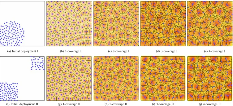
As convergence results we obtain from our extensive exper-iments are all similar, we present only two case to demonstrate the convergence of our algorithm. We consider a targeted area of 1 km2, and initially deploy 100 sensor nodes either at the bottom-left corner (see Fig. 6(a)), or separated into two disjoint groups located at the bottom-left and upper-right
corners (see Fig. 6(f)). According to the following four sub-figures for both cases, our algorithm apparently leads to an “even” node distribution in the sense of multiple coverage. Specifically, in the multiple coverage cases with k = 2,3,4, nodes tend to cluster in groups of size k, in contrast to the pure even distribution fork= 1. This is not a surprise as such an “even clustering” distribution yields more overlaps of the dominating regions among every cluster, which in turn reduces the required sensing range. Interestingly, this appears to also meet the needs of maximumk-coverage. As we discussed in Sec. IV-C, APOLLO leads to a co-location deployment for the extreme example of using three nodes to achieve 3-coverage. The second case also shows that two disconnected clusters will eventually merge into a concocted network. Our extensive simulations show that the initial deployment does not have significant impact on the algorithm output.
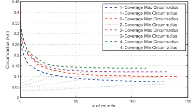
We show the convergence process of APOLLO in Fig. 7. Since a sensor node finally reaches the Chebyshev center of
0 50 100 150 0 0.05 0.1 0.15 0.2 0.25 0.3 0.35 0.4 0.45 # of rounds Circumradius (km)
1−Coverage Max Circumradius 1−Coverage Min Circumradius 2−Coverage Max Circumradius 2−Coverage Min Circumradius 3−Coverage Max Circumradius 3−Coverage Min Circumradius 4−Coverage Max Circumradius 4−Coverage Min Circumradius
Fig. 7. The convergence of APOLLO.
its dominating region and the sensing range is equivalent to the circumradius of the dominating region, we illustrate the relationship between execution rounds (of lengthτ ms each) and the maximum/minimum circumradii. As the nodes are deployed at the corner of the targeted area initially, the max-imum circumcicle usually appears on the network boundary, which is mainly determined by the searching ring (Fig. 3). Consequently, the maximum circumradii fork= 1,2,3,4are almost the same at the beginning. Corresponding to our proof of termination, the maximum circumradius is monotonically decreasing with the execution rounds of APOLLO, while the minimum radius is increasing in general. In the end, the maximum and minimum radii are very close to each other, especially for larger k. While the monotonic decreasing in maximum circumradius shows the termination of APOLLO, the fact that the minimum circumradius coincides with the maximum one further confirms the balanced sensing load. B. Energy Consumption during Deployments
In this section, we use TOSSIM [27] simulations driven by realistic power consumption data to evaluate the energy con-sumption of the whole deployment process. We assume that a mobile sensor node is equipped with a Micromo coreless D-C motor (www.micromo.com/coreless-dc-motors-data-sheets. aspx). It moves a MicaZ Mote in a speed of 0.2 m/s with an energy consumption of 120 mW. We get the communication cost data from the specification of the popular CC2420 radio [1]: transmit power 52.5 mW and receiving (or idle-listening)
(a) Initial deployment I (b) 1-coverage I (c) 2-coverage I (d) 3-coverage I (e) 4-coverage I
(f) Initial deployment II (g) 1-coverage II (h) 2-coverage II (i) 3-coverage II (j) 4-coverage II Fig. 6. Initial deployments andk-coverage (k= 1,2,3,4) deployments as the output of APOLLO.
0 0.1 0.2 0.3 0.4 0.5 0.6 0.7 0.8 0.9 11 0 1000 2000 3000 4000 5000 6000 7000 8000 Step size α Comm. consumption (J) Net 1 Net 2 Net 3 Net 4 Net 5 Net 6 0 0.1 0.2 0.3 0.4 0.5 0.6 0.7 0.8 0.9 11 5500 6000 6500 7000 7500 8000 8500 9000 Step size α Motion consumption (J) Net 1 Net 2 Net 3 Net 4 Net 5 Net 6
(a) Total communication consumption (b) Total motion consumption
0 0.1 0.2 0.3 0.4 0.5 0.6 0.7 0.8 0.9 11 0.7 0.8 0.9 1 1.1 1.2 1.3 1.4 x 10⁴ Step size α Combined consumption (J) Net 1 Net 2 Net 3 Net 4 Net 5 Net 6 0 0.2 0.4 0.6 0.8 1 130 140 150 160 170 180 190 200 210 220 Step size α
Combined node consumption (J)
Net 1 Net 2 Net 3 Net 4 Net 5 Net 6
(c) Total combined consumption (d) Node combined consumption Fig. 8. Energy consumption during the autonomous deployments power 56.4 mW. We assume that, during the i-th round, the radios are disabled when nodes move, and the communication (and computation) session starts only when nodes have moved to their new locations {u+i } (seeAlgorithm 1).
Based on the same scenario studied in Sec. VI-A (i.e., 100 nodes on 1 km2 area), Fig. 8 demonstrates the actual
energy consumption of six autonomous deployments. It is evident that a smaller step size α results in more rounds but shorter total moving distances; this is shown by a decreasing communication consumption in Fig. 8(a) and an increasing motion consumption in Fig. 8(b) as functions ofα. Therefore, given certain power consumption specifications for motion and communication, we may tune αto obtain an energy efficient deployment. For our current settings, the best step size shown by Fig. 8(c) is around 0.3 to 0.7. We also pick up nodes that consume the highest energy in each WSN to illustrate the energy consumed by individual nodes in Fig. 8(d). To put these consumptions into perspective, a 2450mAh Energizer
(www.energizer.com) AA battery contains 13kJ, so the (max-imum) individual node consumption of 200J only accounts from a small part of the node’s energy storage.
We also report the time cost of APOLLO in Fig. 9. As the time cost stems from both communication and motion, the general trend is similar to the total combined consump-tion shown by Fig 8(c): the time cost is minimized around
α∈[0.3,0.7]as well, for which APOLLO terminates within
around 25 minutes and is reasonable for practical applications.
0 0.1 0.2 0.3 0.4 0.5 0.6 0.7 0.8 0.9 1 1200 1400 1600 1800 2000 2200 2400 2600 Step size α Time cost (s) Net 1 Net 2 Net 3 Net 4 Net 5 Net 6
Fig. 9. Total time cost.
C. Energy Consumption after Deployments
In this section, we show the sensing energy consumption after APOLLO completes the deployments. We again consider
20 60 100 140 180 0 0.1 0.2 0.3 0.4 # of nodes
Maximum sensing load
1−Coverage 2−Coverage 3−Coverage 4−Coverage 20 60 100 140 180 0 2 4 6 8 10 # of nodes
Total sensing load
1−Coverage 2−Coverage 3−Coverage 4−Coverage
(a) Maximum sensing load (b) Total sensing load Fig. 10. Energy consumption in the final deployments of 100 nodes a targeted area of 1 km2, while scaling the network size from 20 to 180. As data processing and memory accessing consume
most of power in sensing and their frequency depends on the covered area, we model the energy consumption in sensing to be proportional to the area of the sensing disk centered at the sensor node with a radius ri. In particular, we define the
energy consumption function as E(ri) =πri2: an increasing
function of ri
We illustrate the sensing energy consumption in terms of maximum load max{E(ri)}i=1,...,N and total load
∑N
i=1E(ri) in Fig. 10. As we deploy more sensor nodes to
a given targeted area, each node takes care of less area when achieving a certain coverage. The maximum sensing load is thus decreasing with the increasing number of nodes. Given a certain number of nodes, to achieve higher coverage degree, each sensor node is supposed to cover larger area thereby enhancing the maximum sensing load. We also observe that for k1-coverage andk2-coverage, the ratio of maximum loads
between them is roughly k1/k2, which can be explained as
follows. Since APOLLO makes the minimum sensing range very close to the maximum one, each sensor node roughly covers the same area k|A|/N, i.e., E(ri) = k|A|/N where
|A|is the area of the targeted region. Nevertheless, increasing the number of nodes does decrease the total sensing load of the WSN, shown by Fig. 10 (b). Since using a less number of nodes implies a larger sensing disk for each node, this in turn yields more overlap between sensing ranges (i.e., a larger sensing redundance), thus a higher total load.
D. Comparisons with Min-Nodek-Coverage
As mentioned in Sec. IV-C, our APOLLO algorithm results in a good approximation to min-node k-coverage problem (where all nodes have the same sensing range and the objective is to minimize the number of nodes used to achieve k -coverage). In this section, we compare our algorithm with the deployment strategies proposed in [5] and [3], in terms of the required number of nodes guaranteeing k-coverage (k ≥ 2). As we can increase the minimum sensing range to the maximum one in the output of APOLLO without compromising coverage, we assign an identical sensing range to every node as the maximum sensing range R∗ in our case. Bai et al. have proven in [5] that, without considering boundary effect and with an identical sensing range r, the optimal congruent deployment density4 for 2-coverage is
4π/3√3. Given a targeted area A, we thus compute the minimum number of sensor nodes Nk∗=2 for 2-coverage as:
Nk∗=2 = |A|
4π
3√3
πr2 =
4|A|
3√3R∗2, here we use |A| to replace the area of Voronoi polygons generated by sensor nodes, which leads to an under-estimation of Nk∗=2 due to the boundary effect. We simulate large-scale WSNs with size ranging from 1000 to 1600 in a 1 km2targeted area. The result is shown in Table I. In general, the number of nodes deployed by APOLLO is about 15% higher than the minimum value, and it is obvious that the boundary effect is the main reason for this difference. As the boundary effect is not considered in [5], extra nodes are needed to cover the vacancies on the boundary due to the mismatch between the congruent deployment and an arbitrarily
4Deployment density is defined as a ratio of the area of sensing disks to
the area of Voronoi polygons generated by sensor nodes [5].
shaped targeted area. Therefore, we conclude that APOLLO actually leads to a very good approximation of the min-node 2-coverage problem.
TABLE I
THE MINIMUM NUMBER OF SENSOR NODES TO ACHIEVE2-COVERAGE
N 1000 1200 1400 1600
R∗ (m) 30.35 27.12 25.23 23.57
Nk∗=2 836 1047 1210 1386
In [3], Ammariet al.propose to decompose a targeted area into adjacent Reuleaux triangles, and nodes are deployed in the intersection areas between these triangles (so-called lens in [3]). According to their derivation, 6k|A|
(4π−3√3)r2 nodes are required tok-coverAwherek≥3andris the sensing range. Here we compare this feasible deployment with APOLLO. We deploy 180 nodes in a 1 km2 area and let all nodes have
the same sensing range R∗k. We also compte the number of nodes that deployed according to the strategy proposed in [3] as Nk∗= 6k
(4π−3√3)R∗2
k
. From the results shown in Table II, it is very clear that APOLLO can use much less nodes to achieve the same level of coverage compared with [3].
TABLE II
THE NUMBER OF SENSOR NODES TO ACHIEVEk-COVERAGE WITH THE STRATEGY PROPOSED IN[3]FORk= 3,4, ...,8
k 3 4 5 6 7 8
R∗k (m) 87.6 102.1 112.4 123.6 133.9 143.2
Nk∗ 318 313 323 320 318 318
E. Performance in Maximumk-Coverage
In addition to the analysis in Sec. IV-C, we evaluate the performance of APOLLO in solving maximum k-coverage problem. Due to space limitation, we only illustrate the results of 4-coverage. We assume sensor nodes have fixed sensing ranges of 135m and are deployed in a square targeted region of 1 km2. We also vary the network scale from 80 to 110 with
a step of 10. The 4-coverage ratio (i.e., the ratio between the 4-covered area and the whole targeted region) in each round is demonstrated in Fig. 11. It is shown the area 4-covered by the sensor nodes is increased with the execution of APOLLO, and reaches maximum when APOLLO converges. Since the sensing ranges of the sensor nodes are fixed, a network with s-mall scale may not be able to fully 4-cover the targeted region, e.g., 80, 90 or 100 nodes in our case. By gradually deploying more sensor nodes (e.g., 110 nodes), we can have the whole targeted area 4-covered. Recall that N = 110 sensor nodes with a fixed sensing range of r = 135m can 4-cover (hence
k= 4) an area of up to N(4π−
√ (3))r2
6k = 0.9km
2. Therefore,
we believe that, APOLLO provides a good approximation to the maximumk-coverage problem.
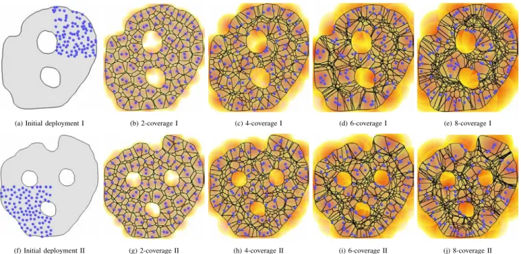
F. Adaptability to Obstacles
We demonstrate the autonomous adaptability of APOLLO to arbitrarily shaped targeted area (with obstacles inside) in
(a) Initial deployment I (b) 2-coverage I (c) 4-coverage I (d) 6-coverage I (e) 8-coverage I
(f) Initial deployment II (g) 2-coverage II (h) 4-coverage II (i) 6-coverage II (j) 8-coverage II Fig. 12. Adaptability of APOLLO to arbitrarily shaped areas and obstacles as well.
0 20 40 60 80 100 120 0.4 0.5 0.6 0.7 0.8 0.9 1 # of rounds 4−coverage ratio 80 nodes 90 nodes 100 nodes 110 nodes
Fig. 11. 4-coverage ratio.
Fig. 12. The “holes” within the network region represent ob-stacles that mobile sensor nodes cannot move upon. Obviously, APOLLO adapts well to these irregularities and again achieves the even clustering distribution as if the area were regular. G. Extension to 3D Surfaces
We apply the 3D APOLLO extension discussed in Sec. V for WSN deployments on various 3D terrain surface models. The three terrain models are approximated by 5k, 20k and 130k triangles, respectively. In Fig. 13, each row shows one terrian where we deploy the sensor nodes. Since a large-scale sensor network are usually air-dropped in the applications of terrain monitoring, we initially deploy 400, 400 and 800 mobile sensor nodes for these three terrains respectively in a random manner. Fig. 13 shows the outputs also reflect clustering distributions in the multiple coverage cases with
k= 2,3,4. The similarity between Fig. 13 and Fig. 6 clearly demonstrates that our deployment algorithm designed for 2D deployments has been successfully extended to handle 3D surface deployments. Considering space limit, we hereby omit the illustration of the convergence process of APOLLO in 3D deployment, as it is very similar to its 2D counterpart.
In Table III, we use the maximum and minimum (Euclidean) sensing ranges resulted from the autonomous deployments to show the quality (in terms of load balancing) of the coverage. In order to make the numbers comparable to each other, we normalize the three surfaces such that their 2D projections are all on a 1 km2area. A direction interpretation,
TABLE III
THE MAXIMUM AND MINIMUM SENSING RANGES FOR THREE SURFACE DEPLOYMENTS
Surface 1 Surface 2 Surface 3
k 2 3 4 2 3 4 2 3 4
Max range 56.77 69.35 81.80 44.94 54.53 55.65 35.56 38.09 47.46
Min range 47.06 62.21 76.97 37.55 46.93 53.32 29.49 31.69 41.45
by comparing Table III with Fig. 7, the differences between the maximum sensing ranges and the minimum sensing ranges in 3D deployments are a little larger than the ones delivered by 2D deployments. In another word, quality of APOLLOs output in terms of load balancing is worse in 3D than in 2D. This is expectable as the problem becomes significantly harder to handle on 3D surfaces. However, the results in Table III do not indicate a worse performance of APOLLO in terms of solving the k-coverage optimization problem, because it has never been proven that an optimal k-coverage solution (for
k > 2) for either 2D planes or 3D surfaces can be or have
to be achieved by disks with an identical radius. It is highly possible that, on 3D surfaces, an optimal k-coverage solution indeed accommodates variable radii. Another reason is that, we employ an approximated Chebyshev centers in 3D APOLLO which may lead to compromise in terms of load balancing.
VII. CONCLUSION
In this paper, we have focused on minimizing the maximum sensing range to achieve load balancing k-coverage through autonomous deployments (i.e., relying on mobile sensors n-odes and the wireless communications among them). We have