Predictive Modeling in Actuarial Science

1

Predictive Modeling in Actuarial Science

Chapter Preview.Predictive modeling involves the use of data to forecast future events. It relies on capturing relationships between explanatory variables and the predicted variables from past occurrences and exploiting them to predict future outcomes. The goal of this two-volume set is to build on the training of actuaries by developing the fundamentals of predictive modeling and providing corresponding applications in actuarial science, risk management, and insurance. This introduction sets the stage for these volumes by describing the conditions that led to the need for predictive modeling in the insurance industry. It then traces the evolution of predictive modeling that led to the current statistical methodologies that prevail in actuarial science today.

1.1 Introduction

A classic definition of an actuary is “one who determines the current financial impact of future contingent events.”1_{Actuaries are typically employed by insurance companies}

who job is to spread the cost of risk of these future contingent events.

The day-to-day work of an actuary has evolved over time. Initially, the work involved tabulating outcomes for “like” events and calculating the average outcome. For example, an actuary might be called on to estimate the cost of providing a death benefit to each member of a group of 45-year-old men. As a second example, an actuary might be called on to estimate the cost of damages that arise from an automobile accident for a 45-year-old driver living in Chicago. This works well as long as there are large enough “groups” to make reliable estimates of the average outcomes.

Insurance is a business where companies bid for contracts that provide future benefits in return for money (i.e., premiums) now. The viability of an insurance company depends on its ability to accurately estimate the cost of the future benefits it promises to provide. At first glance, one might think that it is necessary to obtain data

1 _{Attributed to Frederick W. Kilbourne.}

2 Predictive Modeling in Actuarial Science

from sufficiently large groups of “like” individuals. But when one begins the effort of obtaining a sufficient volume of “like” data, one is almost immediately tempted to consider using “similar” data. For example, in life insurance one might want to use data from a select group of men with ages between 40 and 50 to estimate the cost of death benefits promised to a 45-year-old man. Or better yet, one may want to use the data from all the men in that age group to estimate the cost of death benefits for all the men in that group. In the automobile insurance example, one may want to use the combined experience of all adult men living in Chicago and Evanston (a suburb north of Chicago) to estimate the cost of damages for each man living in either city arising from an automobile accident.

Making use of “similar” data as opposed to “like” data raises a number of issues. For example, one expects the future lifetime of a 25-year-old male to be longer that of a 45-year-old male, and an estimate of future lifetime should take this difference into account. In the case of automobile insurance, there is no a priori reason to expect the damage from accidents to a person living in Chicago to be larger (or smaller) than the damage to a person living in Evanston. However, the driving environment and the need to drive are quite different in the two cities and it would not be prudent to make an estimate assuming that the expected damage is the same in each city.

The process of estimating insurance costs is now called “predictive modeling.”2 In a very real sense, actuaries had been doing “predictive modeling” long before the term became popular. It is interesting to see how the need for predictive modeling has evolved in the United States.

In 1869, the U.S. Supreme Court ruled inPaulv. Virginiathat “issuing a policy of insurance is not a transaction of commerce.” This case had the effect of granting antitrust immunity to the business of insurance. As a result, insurance rates were controlled by cartels whose insurance rates were subject to regulation by the individual states. To support this regulation, insurers were required to report detailed policy and claim data to the regulators according to standards set by an approved statistical plan. The Supreme Court changed the regulatory environment in 1944. InUnited States v. Southeast Underwriters Association it ruled that federal antitrust law did apply under the authority of the Commerce Clause in the U.S. Constitution. But by this time, the states had a long-established tradition of regulating insurance companies. So in response, the U.S. Congress passed the McCarran-Ferguson Act in 1945 that grants insurance companies exemption from federal antitrust laws so long as they are regulated by the states. However, the federal antitrust laws did apply in cases of boycott, coercion, and intimidation.

The effect of the McCarran-Ferguson Act was to eliminate the cartels and free the insurers to file competitive rates. However, state regulators still required the insurers

to compile and report detailed policy and claim data according to approved statistical plans. Industry compilations of these data were available, and insurance companies were able to use the same systems to organize their own data.

Under the cartels, there was no economic incentive for a refined risk classification plan, so there were very few risk classifications. Over the next few decades, insurance companies competed by using these data to identify the more profitable classes of insurance. As time passed, “predictive modeling” led to more refined class plans.

As insurers began refining their class plans, computers were entering the insurance company workplace. In the 60 s and 70 s, mainframe computers would generate thick reports from which actuaries would copy numbers onto a worksheet, and using at first mechanical and then electronic calculators, they would calculate insurance rates. By the late 70 s some actuaries were given access to mainframe computers and the use of statistical software packages such asSAS. By the late 80 s many actuaries had personal computers with spreadsheet software on their desks.

As computers were introduced into the actuarial work environment, a variety of data sources also became available. These data included credit reports, econometric time series, geographic information systems, and census data. Combining these data with the detailed statistical plan data enabled many insurers to continue refining their class plans. The refining process continues to this day.

1.2 Predictive Modeling and Insurance Company Operations

Although actuarial predictive modeling originated in ratemaking, its use has now spread to loss reserving and the more general area of product management. Specifi-cally, actuarial predictive modeling is used in the following areas:

r Initial Underwriting. As described in the previous section, predictive modeling has its actuarial roots in ratemaking, where analysts seek to determine the right price for the right risk and avoid adverse selection.

r Renewal Underwriting. Predictive modeling is also used at the policy renewal stage where the goal is to retain profitable customers.

r Claims Management. Predictive modeling has long been used by actuaries for (1) managing claim costs, including identifying the appropriate support for claims-handling expenses and detecting and preventing claims fraud, and for (2) understanding excess layers for reinsurance and retention.

r Reserving. More recently predictive modeling tools have been used to provide manage-ment with an appropriate estimate of future obligations and to quantify the uncertainty of the estimates.

As the environment became favorable for predictive modeling, some insurers seized the opportunity it presented and began to increase market share by refining their risk

4 Predictive Modeling in Actuarial Science 1990 1993 1996 1999 2002 2005 2008 50+ 10−50 Top 10 0 20 40 60 80 100 300 350 400 450 500 550 Count

Fig. 1.1. Growth in market share by large insurers. The bar chart shows the percent-age, on the left-hand vertical axis, of personal automobile premiums written by the top 10 insurers (in terms of premium volume), the next 40, and other insurers. The right-hand vertical axis shows the decreasing number of insurer groups over time, as indicated by the dashed line.Source: ISO.

classification systems and “skimming the cream” underwriting strategies. Figure 1.1 shows how the top American insurers have increased their market share over time. It was this growth in market share that fueled the growth in predictive modeling in insurance.

Actuaries learn and develop modeling tools to solve “actuarial” problems. With these tools, actuaries are well equipped to make contributions to broader company areas and initiatives. This broader scope, sometimes known as “business analytics,” can include the following areas:

rSales and Marketing – these departments have long used analytics to predict customer behavior and needs, anticipate customer reactions to promotions, and to reduce acqui-sition costs (direct mail, discount programs).

rCompensation Analysis – predictive modeling tools can be used to incentivize and reward appropriate employee/agent behavior.

rProductivity Analysis – more general than the analysis of compensation, analytic tools can be used to understand production by employees and other units of business, as well as to seek to optimize that production.

rFinancial Forecasting – analytic tools have been traditionally used for predicting finan-cial results of firms.

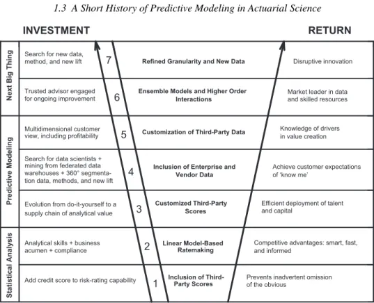
Predictive modeling in the insurance industry is not an exercise that a small group of actuaries can do by themselves. It requires an insurer to make significant investments in their information technology, marketing, underwriting, and actuarial functions. Figure 1.2 gives a schematic representation of the investments an insurer has to make.

Next Big Thing

Predictive Modeling

Statistical Analysis

INVESTMENT RETURN

Search for new data, method, and new lift

Trusted advisor engaged for ongoing improvement

Multidimensional customer view, including profitability

Search for data scientists + mining from federated data warehouses + 360° tion data, methods, and new lift

Evolution from do-it-yourself to a supply chain of analytical value

Analytical skills + business acumen + compliance

Add credit score to risk-rating capability

7 6 5 4 3 2 1

Refined Granularity and New Data

Ensemble Models and Higher Order Interactions

Customization of Third-Party Data

Inclusion of Enterprise and Vendor Data Customized Third-Party Scores Linear Model-Based Ratemaking Inclusion of Third- Party Scores Disruptive innovation

Market leader in data and skilled resources

Knowledge of drivers in value creation

Achieve customer expectations of ‘know me’

Efficient deployment of talent and capital

Competitive advantages: smart, fast, and informed

Prevents inadvertent omission of the obvious

Fig. 1.2. Investing in predictive modeling.Source: ISO.

1.3 A Short History of Predictive Modeling in Actuarial Science

We would like to nominate the paper “Two Studies in Automobile Insurance Ratemak-ing” by Bailey and Simon (1960) as the initiator of the modern era of predictive modeling in actuarial science.3In this paper, they addressed the problem of classi-fication ratemaking. They gave the example of automobile insurance that has five use classes cross-classified with four merit rating classes. At that time, rates for use classes and merit rating classes were estimated independently of each other. They started the discussion by noting that the then current methodology “does not reflect the relative credibility of each subgroup and does not produce the best fit to the actual data. Moreover, it produces differences between the actual data and the fitted values which are far too large to be caused by chance.” They then proposed a set of criteria that an “acceptable set of relativities” should meet:

(1) “It should reproduce the experience for each class and merit rating class and also the overall experience; i.e., bebalancedfor each class and in total.”

(2) “It should reflect the relativecredibilityof the various groups involved.”

(3) “It should provide a minimum amount of departure for the maximum number of people.”

6 Predictive Modeling in Actuarial Science

(4) “It should produce a rate for each subgroup of risk which is close enough to the experience so that the differences could reasonably be caused bychance.”

Bailey and LeRoy then considered a number of models to estimate the relative loss ratios, rij, for use class i and merit rating class j. The two most common models they considered were the additive modelrij =αi+βj and the multiplicative modelrij =αi·βj. They then described some iterative numerical methods to estimate the coefficients {αi} and{βj}. The method that most insurers eventually used was described a short time later by Bailey (1963) in his paper titled “Insurance Rates with Minimum Bias.” Here is his solution for the additive model:

(1) Calculate the initial estimates,

βj =

i

nij ·rij

for each j. For the additive model, Bailey used the weights, nij, to represent the

exposure measured in car years.

(2) Given the “balanced” criterion (#1 above) for eachi, we have that

j

nij·(rij−αi−βj)=0.

One can solve the above equation for an estimate of eachαi,

αi = jnij(rij−βj) jnij .

(3) Given the estimates{αi}, similarly calculate updated estimates ofβj:

βj =

inij(rij−αi) inij

.

(4) Repeat Steps 2 and 3 using the updated estimates of{αi}and{βj}until the estimates

converge.

This iterative method is generally referred to as the Bailey minimum bias additive model. There is a similarly derived Bailey minimum bias multiplicative model. These models can easily be generalized to more than two dimensions.

As mentioned in the description of the iterative method, the “balance” criterion is met by the design of the method. The method meets the “credibility” criterion because its choice of weights are equal to the exposure. To satisfy the “minimum departure” or “goodness of fit” (in current language) criterion, Bailey and Simon recommended testing multiple models to see which one fit the best. They proposed using the chi-square statistic to test if the differences between actual and fitted were “due to chance.” Although their technology and language were different from now, they were definitely thinking like current actuarial modelers.

The Bailey minimum bias models were easy to program inFORTRANandBASIC, the predominant computer programming languages of the sixties and seventies, and they were quickly adopted by many insurers. We did a quick poll at a recent Casualty Actuarial Society seminar and found that some insurers are still using these models.

Meanwhile, statisticians in other fields were tackling similar problems and devel-oping general statistical packages.SPSSreleased its first statistical package in 1968. Minitabwas first released in 1972.SAS released the first version of its statistical package in 1976. The early versions of these packages included functions that could fit multivariate models by the method of least squares.

Let’s apply the least squares method to the previous example. Define B =

i,j

nij ·(rij −αi−βj)2.

To find the values of the coefficients{αi}and{βj}that minimizeB we set ∂B ∂αi = 2 j nij ·(rij−αj −βj) =0 for alli and ∂B ∂βj = 2 j nij ·(rij−αi−βj)=0 for allj.

These equations are equivalent to the “balance” criterion of Bailey and Simon. The Bailey minimum bias additive model and the least square method differ in how they solve for the coefficients {αi} and{βj}. Bailey uses an iterative numerical solution, whereas the statistical packages use an analytic solution.

Recognizing that the method of least squares is equivalent to maximum likeli-hood for a model with errors having a normal distribution, statisticians developed a generalization of the least squares method that fit multivariate models by maximum likelihood for a general class of distributions. The initial paper by Nelder and Wed-derburn (1972) was titled “Generalized Linear Models.” The algorithms in this paper were quickly implemented in 1974 with a statistical package called GLIM, which stands for “Generalized Linear Interactive Modeling.” The second edition of McCul-lagh and Nelder’s book Generalized Linear Models(MacCullagh and Nelder 1989) became the authoritative source for the algorithm that we now call a GLM.

Brown (1988) was the first to compare the results of the Bailey minimum bias models with GLMs produced by the GLIM package.4 The connection between GLMs and Bailey minimum bias models was further explored by Venter (1990),

4 _{Brown attributes his introduction to GLMs to Ben Zehnwirth and Piet DeJong while on a sabbatical leave in} Australia.

8 Predictive Modeling in Actuarial Science

Zehnwirth (1994), and then a host of others. The connection between GLMs and Bai-ley minimum bias models reached its best expression in Mildenhall (1999). For any given GLM model there is a corresponding set of weights{wij}, (given by Mildenhall’s Equation 7.3) for which

i

wij ·(rij−μij)=0 for alli and

j

wij ·(rij −μij)=0 for allj.

As an example one can setμij =αi+βj and there is a GLM model for which the corresponding set of weights{wi,j} = {nij}yields the Bailey additive model. If we set μij =αi·βj there is a GLM model for which the corresponding set of weights{wij} yields the Bailey multiplicative model. Other GLM models yield other minimum bias models.

The strong connection between the Bailey minimum bias models and the GLM models has helped make the actuarial community comfortable with GLMs. The actu-arial community is rapidly discovering the practical advantages of using statistical packages such asSASandR. These advantages include the following:

rthe ability to include continuous variables (such as a credit score) in the rating plan

rthe ability to include interactions among the variables in the rating plan

rthe diagnostic tools that allow one to evaluate and compare various models

As a result, the leading edge of actuarial scientists are now using statistical packages for their predictive modeling tasks.

As described in Section 1.2, these tasks go beyond the classification ratemaking applications discussed earlier. Loss reserving is another important task typically per-formed by actuaries. An early reference to loss reserving that reflects the statistical way of thinking is found in Taylor (1986). Since then there have been several papers describing statistical models in loss reserving. We feel that the papers by Mack (1994), Barnett and Zehnwirth (2000), and England and Verrall (2002) represent the different threads on this topic. These papers have led to a number of specialized loss reserving statistical packages. Although some packages are proprietary, theR chainladder package is freely available.

1.4 Goals of the Series

In January 1983, the North American actuarial education societies (the Society of Actuaries and the Casualty Actuarial Society) announced that a course based on regression and time series would be part of their basic educational requirements. Since that announcement, a generation of actuaries has been trained in these fundamental applied statistical tools. This two-set volume builds on this training by developing

the fundamentals of predictive modeling and providing corresponding applications in actuarial science, risk management, and insurance.

Predictive modeling involves the use of data to forecast future events. It relies on capturing relationships between explanatory variables and the predicted variables from past occurrences, and exploiting those relationships to predict future outcomes. This two-set volume emphasizes life-long learning by developing predictive modeling in an insurance and risk management context, providing actuarial applications, and introducing more advanced statistical techniques that can be used by actuaries to gain a competitive advantage in situations with complex data.

Volume 1 lays out the foundations of predictive modeling. Beginning with reviews of regression and time series methods, this book provides step-by-step introductions to advanced predictive modeling techniques that are particularly useful in actuarial practice. Readers will gain expertise in several statistical topics, including generalized linear modeling and the analysis of longitudinal, two-part (frequency/severity), and fat-tailed data. Thus, although the audience is primarily professional actuaries, we have in mind a “textbook” approach, and so this volume will also be useful for continuing professional development where analytics play a central role.

Volume 2 will examine applications of predictive models, focusing on property and casualty insurance, primarily through the use of case studies. Case studies provide a learning experience that is closer to real-world actuarial work than can be provided by traditional self-study or lecture/work settings. They can integrate several analytic techniques or alternatively can demonstrate that a technique normally used in one practice area could have value in another area. Readers can learn that there is no unique correct answer. Practicing actuaries can be exposed to a variety of techniques in contexts that demonstrate their value. Academic actuaries and students will see that there are multiple applications for the theoretical material presented in Volume 1.

References

Bailey, R. A. (1963). Insurance rates with minimum bias.Proceedings of the Casualty Actuarial Society Casualty Actuarial Society L, 4.

Bailey, R. A. and L. J. Simon (1960). Two studies in automobile insurance ratemaking. Proceedings of the Casualty Actuarial Society XLVII, 192–217.

Barnett, G. and B. Zehnwirth (2000). Best estimates for reserves.Proceedings of the Casualty Actuarial Society LXXXVII, 245–321.

Brown, R. A. (1988). Minimum bias with generalized linear models.Proceedings of the Casualty Actuarial Society LXXV, 187.

England, P. and R. Verrall (2002). Stochastic claims reserving in general insurance.Institute of Actuaries and Faculty of Actuaries 28.

MacCullagh, P. and J. A. Nelder (1989).Generalized Linear Models(2nd ed.). Chapman and Hall/CRC Press.

Mack, T. (1994). Measuring the variability of chain ladder reserve estimates. InCasualty Actuarial Society Forum.

10 Predictive Modeling in Actuarial Science

Mildenhall, S. J. (1999). A systematic relationship between minimum bias and generalized linear models.Proceedings of the Casualty Actuarial Society LXXXVI, 393.

Nelder, J. A. and R. W. Wedderburn (1972). Generalized linear models.Journal of the Royal Statistical Society. Series A (General), 370–384.

Taylor, G. C. (1986).Claims Reserving in Non-Life Insurance. Elsevier Science Publishing Company, Inc.

Venter, G. G. (1990). Minimum bias with generalized linear models [discussion]. Proceedings of the Casualty Actuarial Society LXXVII, 337.

Zehnwirth, B. (1994). Ratemaking: From Bailey and Simon [1960] to generalized linear regression models. InCasualty Actuarial Society Forum, 615.