Intermediate-Complexity Biological Modeling Framework for Nutrient Cycling in Lakes Based on Physical Structure

Utah State University Utah State University

DigitalCommons@USU

DigitalCommons@USU

All Graduate Plan B and other Reports Graduate Studies

2009

Intermediate-Complexity Biological Modeling Framework for

Intermediate-Complexity Biological Modeling Framework for

Nutrient Cycling in Lakes Based on Physical Structure

Nutrient Cycling in Lakes Based on Physical Structure

Michael Clay Rigley

Utah State University

Follow this and additional works at: https://digitalcommons.usu.edu/gradreports Part of the Applied Mathematics Commons

Recommended Citation Recommended Citation

Rigley, Michael Clay, "Intermediate-Complexity Biological Modeling Framework for Nutrient Cycling in Lakes Based on Physical Structure" (2009). All Graduate Plan B and other Reports. 1249.

https://digitalcommons.usu.edu/gradreports/1249

This Report is brought to you for free and open access by the Graduate Studies at DigitalCommons@USU. It has been accepted for inclusion in All Graduate Plan B and other Reports by an authorized administrator of DigitalCommons@USU. For more information, please contact [email protected].

Intermediate-Complexity Biological Modeling Framework for Nutrient Cycling in

Lakes Based on Physical Structure

by

Michael Clay Rigley

A report submitted in partial fulfillment of the requirements for the degree

of

MASTER OF SCIENCE m

Applied Mathematics

UTAH STATE UNIVERSITY Logan, Utah

An Intermediate-Complexity Biological Modeling Framework for Nutrient Cycling

in Lakes Based on Physical Structure

Michael C. Rigley and James Powell

Department of Mathematics and Statistics, Utah State University, Logan UT 84322

James Haefner

Department of Biology, Utah State University, Logan UT 84322

March 11, 2009

Key Words:

total dissolved nitrogen

, seston, nutrient cycling

, compartment model, plunge, Bull

Trout Lake, multi-compartment model

Abstract

Mathematical models for the change in concentration of total dissolved nitrogen (TDN) in mountain lakes are developed based on the dynamics of coupled, well-mixed containers. Each includes a stratified lake structure without the complexity of a full fluid model. A lake is divided into a suite of compartments based on physical structure: warm upper layer ( epilirnnion), cold inflow and insertion layer (metalirnnion), cold lower layer (hypolirnnion), and a warm shallow shelf. With the compartments as the framework and literature values for uptake rates, death rates, half-saturation constants, and sinking rates, systems of equations are written for three models. The first is a system of differential equations including nutrient cycling within each compartment , including changes in TDN due to growth and death of seston as well as loss to and gain from lake sediments. With the literature values, flows, and TDN data taken at the inflow (Baker and Wurtsbaugh 2008), these equations are solved numerically to determine the concentration of

TON in each compartment. The second is a simplified version of the first model containing only fluxes of TON between compartments and the flux in lake sediments. The third is a system of equations for the steady states of the first model found by making an assumption on the half-saturation constant. With TON data taken at the outflow in 2002 (Baker and Wurtsbaugh 2008), terms of sedimentation fluxes are chosen to minimize the sum of the squared difference between the measured and predicted concentrations of TON for each of the three systems. Each model is tested against data taken in 2003 (Baker and Wurtsbaugh 2008). The second model predicts observed TON well in a stratified lake structure without the computational difficulty of a full fluid model. To determine the flows between compartments we solved differential equations for the transport of nutrients into lakes by cold plunging inflows (Hauenstein and Oracos 1984 ). The entrainment rates are treated as eigenvalues, and an eigenvalue problem is solved for the plunging inflow based on discharge data taken in 2003 (Arp 2006) and data taken from a field study on Bull Trout Lake (BTL) in central Idaho in June 2008. The results show that lake structure is a significant factor in relating input and output concentrations of TON.

1 Introduction

Mountain lakes play an important role in ecosystem function and management. As major stopping points for transport of nutrients and pollutants in a drainage basin (i.e. watershed), lakes are natural accumulators and bio-reactors. They play a significant role in uptake and distribution of nutrients in the run off,

primary production by phytoplankton at the base of the food chain, and check points for water quality. Lakes attenuate nutrient pulses, serving some times as nutrient sources, other times as sinks (Wurtsbaugh et al. 2005). From these mixing pots a certain amount of the nutrients and pollutants flow downstream affecting further ecosystems and entering public water supplies. As charismatic and accessible landscape features, mountain lakes are a touchstone for recreation and public perception of ecosystem health. Use of models to predict nutrient transport in these lakes can therefore impact a variety of research enterprises, from basic biological and ecosystem processes to water management and climate scenario exploration.

Although more attention is given to man-made reservoirs and oceans, in recent years, natural lakes have garnered more attention due to some of their unique hydrological dynamics (Fleenor 2000). Cold mountain input streams have a higher density than warmer lake water, and therefore plunge beneath the ambient lake water. This higher density current continually loses density as it entrains ambient lake water and eventually becomes neutrally buoyant with the lake water at which point the current inserts into the middle layer of the lake (Fleenor 2000). In this paper we address the question of the significance of mountain lake structure on the nutrient cycling through mountain lakes and the relative effect of biological activity on nutrients cycling through lakes.

Several models have been created for the nutrient cycling within natural lakes. The full complexity of fluid motions within a lake can be predicted using the Navier-Stokes equations with Boussinesq (NSB) approximation for buoyancy. Nutrient concentrations and population processes can be treated as Lagrangian variables carried with the flow (see, for example, DYRESM at the University of Western Australia or the Hydrodynamic and Water Quality Model at Portland State University (lmberger 1981)). Obtaining the solution of the NSB is computationally intensive and data requirements at the boundaries (lake bottom topography, surface wind forcing and radiative flux) are large. Such models are framed as partial differential equations and biological parameters are treated as continuous functions of temperature and flow parameters, vastly complicating parameter estimation.

Simpler models include a single well-mixed container, essentially a chemostat (Wurtsbaugh 2005). Unfortunately most lakes are not well-mixed; solar input warms the upper layers ( epilirnnion), creating a vertical stratification of temperature and inhibiting vertical mixing. Cold, dense mountain input streams plunge beneath the warmer lake water. The higher density current continually loses density as it entrains lake water and eventually becomes neutrally buoyant, at which point the current inserts into the middle layer, metalirnnion, of the lake (Fleenor 2000). Vertical mixing then occurs between the metalirnnion and the epilirnnion. At Bull Trout Lake (BTL) in Central Idaho part of the flow rises into the epilirnnion where it crosses a shallow shelf, where nutrients are lost and gained from lake sediments before

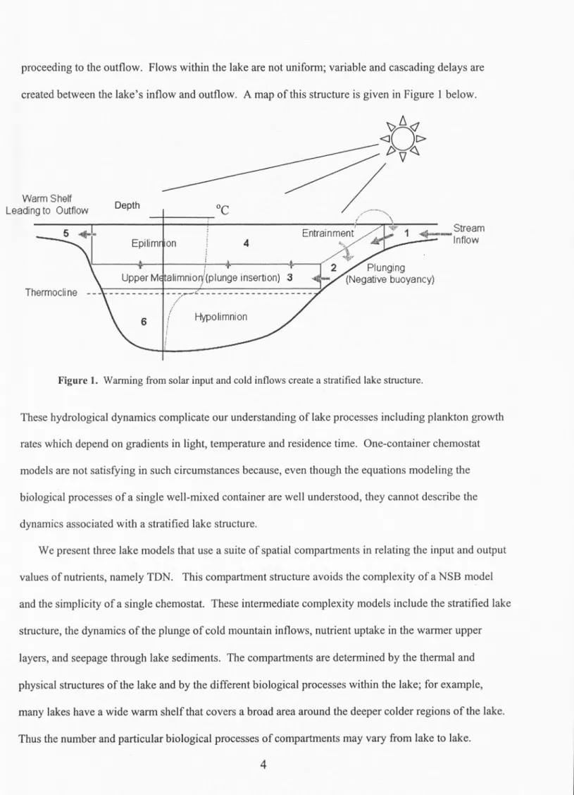
proceeding to the outflow. Flows within the lake are not uniform; variable and cascading delays are created between the lake's inflow and outflow. A map of this structure is given in Figure I below.

Warm Shelf Leading to Outflow Thermocli ne -Depth

oc

·on 4

Entrainm

,:~,J!'

1

--

:~~m

--

---

-

----

,

~

--<"

2 Plunging 3 (Negative buoyancy) .. ···- ,,,· Hypolimnion

Figure 1. Warming from solar input and cold inflows create a stratified lake structure.

These hydrological dynamics complicate our understanding of lake processes including plankton growth rates which depend on gradients in light, temperature and residence time. One-container chemostat models are not satisfying in such circumstances because, even though the equations modeling the biological processes of a single well-mixed container are well understood, they cannot describe the dynamics associated with a stratified lake structure.

We present three lake models that use a suite of spatial compartments in relating the input and output values of nutrients, namely TDN. This compartment structure avoids the complexity of a NSB model and the simplicity of a single chemostat. These intermediate complexity models include the stratified lake structure, the dynamics of the plunge of cold mountain inflows, nutrient uptake in the warmer upper layers, and seepage through lake sediments. The compartments are determined by the thermal and physical structures of the lake and by the different biological processes within the lake; for example, many lakes have a wide warm shelf that covers a broad area around the deeper colder regions of the lake. Thus the number and particular biological processes of compartments may vary from lake to lake.

The study lake, BTL, like many mountain lakes, has a single large input stream which carries

nutrients and plunges below the surface of the lake. The inflow, while entraining some lake water, flows over a small delta that extends into the lake until it plunges down a steep slope at the end of the delta, picking up both vertical and horizontal entrainment from the ambient lake water.

For BTL a suite of three compartments is constructed. The first compartment is made up of the upper regions of the lake or epilirnnion; it is assumed to be about 2m deep based on the warm shelf that extends

around the lake; the second compartment is determined by the dynamics of the inflow- the end of the

plunge is assumed to be near the sharp gradient in the stratification of the temperature of the lake (thermocline). The thermocline was observed at varying depths (between 2 and 6m) at different times

during the day, so compartment 2 is determined by taking the upper and lower bounds observed for the

therrnocline; there is assumed to be no vertical mixing with the lower layer (hypolirnnion) of the lake

(below 6m) where little growth occurs due to lack of sunlight; compartment 3 represents the shallow shelf at BTL where seepage from sediments, groundwater, and other small mountain inlets are included.

For this compartment structure three models are created and tested. Each predicts the concentration of total dissolved nitrogen (TDN) at the outflow given the concentration at the inflow. Total dissolved

nitrogen consists of dissolved inorganic nitrogen, including ammonium (NH4 +), nitrate (NO3

l

and nitrite

(NO2-), and dissolved organic nitrogen, including amino acids, proteins, urea, and humic and fulvic acids (Bronk 2000).

The first model is a biological model including the nutrient cycling between total dissolved nitrogen and seston. Seston is defined as minute particulate material moving in water that is composed of both living organisms, such as plankton, and non-living matter such as plant debris and soil particles (NOAA's

Coral Reef Information System, <<http:coris.noaa.gov/glossary/glossary _l_ z.htrnl>> ). The equations for

each compartment include growth and death rates, half saturation constants, sinking rates, and flux rates

in lake sediments. The concentrations ofTDN and seston within each of the several compartments are

connected by fluxes based on the flow rates between the compartments, thus creating a coupled system of equations for the entire lake. With input values of initial concentration of TDN, seston, and literature

values for growth rates, death rates, half-saturation constants and sinking rates this system of differential equations is solved numerically to determine the concentration of TON and seston in each compartment in terms of time.

The second model is a model of the flux of TON between the lake compartments independent of seston, but still including terms of flux from lake sediments. This model is formed by removing the terms of seston from the first model. This simpler system of differential equations is also solved numerically given input data of the flows between compartments and initial concentrations of TON.

The third model is a model of the steady states of the second model. Setting the changes in concentration of TON to zero, the second model becomes a homogeneous system of linear equations which is solved by row-reduction and back substitution for the steady states. This steady state analysis captures a general relationship between inflow and the outflow in terms of the concentration of TON from lake sediments.

In each model, the terms of flux in lake sediments are determined by minimizing the sum of the squares of the differences between measured and predicted concentration values of TON. The terms of flux in sediments are determined using data taken in 2002 (Baker and Wurtsbaugh 2008). The resulting models are then tested against data taken in 2003 (Baker and Wurtsbaugh 2008).

Given the optimal seepage and entrainment rates, each model predicts the concentration of TON at the outflow of the lake. Each model allows the possibility of a stratified lake structure and the effects from seepage from lake sediments and other mountain inlets without the complexity of a full fluid model. The models are of varying levels of complexity from a simple linear system to a non-linear system of differential equations. The results show that the lake structure is significant in determining the cycling of TON within the lake.

The hydrological dynamics of the lake are represented by the integral models of momentum and buoyancy- dominated regions as constructed by Hauenstein and Oracos ( 1984). When a stream first enters a lake, the force of the stream displaces the lake water near the inflow while entraining some lake water. This is called the momentum-dominated region. After entering the lake the density differences

between the stream and lake waters, and the slope of the lake bed cause the inflow to plunge beneath the warmer lake water. This is defined as the buoyancy-dominated region. We use this basic mathematical framework to determine the flows between compartments in the three models, and the amount of nutrients being cycled within the lake through entrainment.

We solve the differential equations of the momentum-dominated region analytically, while the equations for the buoyancy-dominated region are solved numerically to determine the height (h), breadth

(b), and velocity (u) of the plunge in terms of the distance from the inflow. The flow rates (q

= ubh)

between the compartments of the lake are then determined assuming conservation of volume. These flow rates between compartments are the backbone of the three compartment models.

To test the flow model, measurements were taken as part of a field study at BTL in June 2008. The initial height, width, and breadth of the inflow, some measurements near the insertion point, and general observations were made to fit the flow model. With these measurements, the horizontal and vertical entrainment rates are treated as eigenvalues and are used to match the initial conditions of the height, breadth and velocity of the plunge. The flows from the fit model are then used in the three compartment models.

2 Compartment Model

2.1 Compartments

To predict the flow of nutrients through the lake, we choose compartments to isolate particular biological processes to specific parts of the lake. To determine the compartments several factors are considered. Does the lake morphometry suggest natural compartments like shallow or deeper shelves, deeper regions, or sharp inclines? Does the thermal structure based on sunlight naturally separate warmer inhabitable regions from colder, uninhabitable regions? Do the flows near the inflow or outflow or other lake inlets suggest any currents or structure?

The morphometry of Bull Trout Lake (Figure 2) does show a shallow shelf (0-2m) that extends all around the lake, especially on the northwestern side and near the outflow on the northeast side. There is a

sharp incline near the inflow at the end of the delta. The thermal structure of the lake was measured throughout the lake and the thermocline was calculated at different depths at different points and at different times during the day. Near the inflow, the thermocline was observed to vary between about 2m and 6m. The discharge at the outflow was often measured to be greater than the discharge at the inflow suggesting a significant amount of water entering the lake from sources other than the inflow. There are numerous small unmeasured inflows around the lake as well as groundwater coming through the lake bed.

N

BTL Lake Morphometry

810m

Figure 2. Contour map of BTL. The lake flow from south to north, has a large shallow shelf along the northwestern side of the lake, a delta that runs about 23 meters into the lake, and a maximum depth of about 16 meters.

All of these factors are considered in determining the compartments to BTL. A three compartment model is formed based on the above observations . The first compartment, from the surface to the shallow limit of the thermocline, is chosen to be 2m deep. It includes the volume of water not intersecting the lake bottom, except along the eastern and western boundaries. The second compartment is determined by the measurements of the plunge near the inflow. The thermocline depth was measured to vary from 2 to 6 meters throughout the day, so the second compartment is determined as the region of the lake between 2 and 6 m. This compartment can be thought of as a mixing layer or the layer into which most of the stream sediment initially enters before sinking or rising to other compartments. The third compartment is

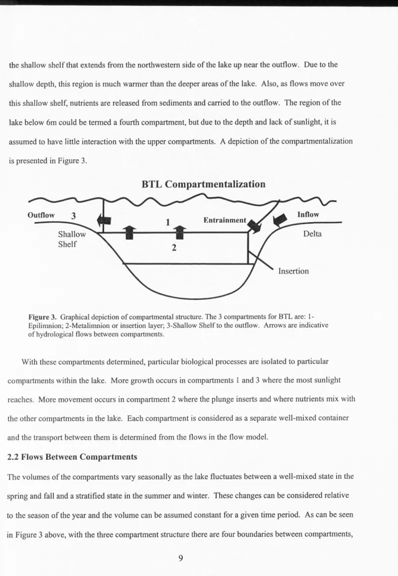
the shallow shelf that extends from the northwestern side of the lake up near the outflow. Due to the shallow depth, this region is much warmer than the deeper areas of the lake. Also, as flows move over this shallow shelf, nutrients are released from sediments and carried to the outflow. The region of the lake below 6m could be termed a fourth compartment, but due to the depth and lack of sunlight, it is assumed to have little interaction with the upper compartments. A depiction of the compartmentalization is presented in Figure 3. Outflow

₃

Shallow Shelf

BTL Compartmentalization

Delta Insertion

Figure 3. Graphical depiction of compartmental structure. The 3 compartments for BTL are: 1-Epilimnion; 2-Metalimnion or insertion layer; 3-Shallow Shelf to the outflow. Arrows are indicative of hydrological flows between compartments.

With these compartments determined, particular biological processes are isolated to particular compartments within the lake. More growth occurs in compartments l and 3 where the most sunlight reaches. More movement occurs in compartment 2 where the plunge inserts and where nutrients mix with the other compartments in the lake. Each compartment is considered as a separate well-mixed container and the transport between them is determined from the flows in the flow model.

2.2 Flows Between Compartments

The volumes of the compartments vary seasonally as the lake fluctuates between a well-mixed state in the spring and fall and a stratified state in the summer and winter. These changes can be considered relative to the season of the year and the volume can be assumed constant for a given time period. As can be seen in Figure 3 above, with the three compartment structure there are four boundaries between compartments,

making 4 flow rates between compartments: the inflow rate (q02) , connecting the input stream with compartment 2; the entrainment rate from compartment l into compartment 2 (q12); the vertical flow rate from compartment 2 to compartment l (q21

=

q02 + q 12); and the flow from compartment 1 to compartment 3 (q13

=

q02). The outflow is the same value as q02 since the volume in compartment 3 must be conserved.

These flow rates determine the flux of nutrients between the three compartments of the lake. Since the volume of each compartment is conserved, the measured outflow on each day is used as the inflow to account for water from sources other than the inflow. The flow rates for the model are determined by solving the system of equations of Hauenstein and Oracos (HOE). The solution for the flow model is given in Section 3.

2.3 Definition of Variables

We now treat each compartment as a well-mixed container, connected by the flow rates. For each model, equations are written for each compartment and the equations are connected by the flow rates between them. The terms are defined in relation to the first model and the second and third models are then derived from the first model.

For each compartment (i

=

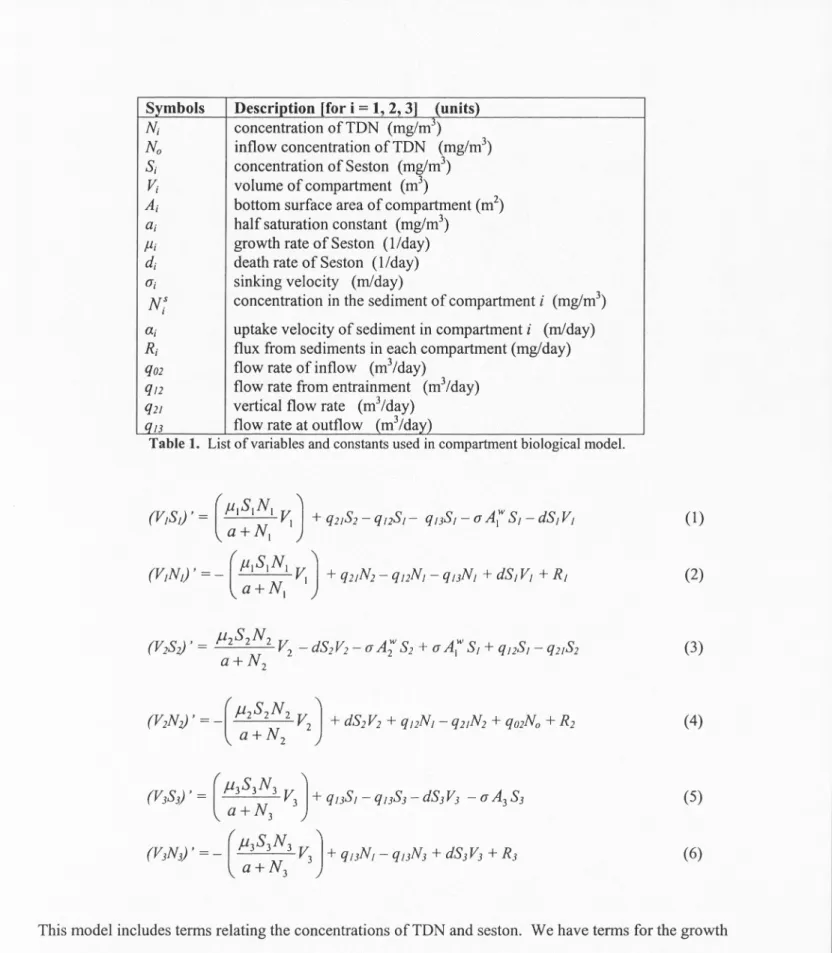
1,2,3) we have the concentration of seston (S;) and TON (N;) in mg/m3, the volume (V;) and bottom surface area (A;) in m3 and m2 respectively , half saturation constants for TON uptake by seston (a;) in mg/m3, growth rates(µ;), death rates (d;), sinking velocities (a;) in rn/day, velocities at which nutrients are released from lake sediments in each compartment (a;) in rn/day, TON flux from sediments in each compartment(R ;

=

a;N

;'

A

;

)

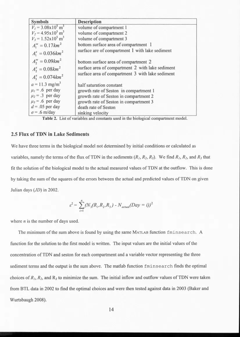
in mg/day, and the flow rates between compartments (from compartment i to}, q02, q21, q,2, q13). A list of these parameters is given below (Table l).

2.4 Model 1 - Biological Compartment Model

Symbols

a;

NS

l

Description [for i

=

1, 2, 3] (units) concentration of TDN (mg/m3)

inflow concentration of TDN (mg/m3)

concentration of Seston ( mg/m3)

volume of compartment (m3)

bottom surface area of compartment (m2)

half saturation constant (mg/m3)

growth rate of Seston (1/day) death rate of Seston (1/day) sinking velocity (rn/day)

concentration in the sediment of compartment i (mg/m3)

uptake velocity of sediment in compartment i (rn/day) flux from sediments in each compartment (mg/day) flow rate of inflow (m3/day)

flow rate from entrainment (m3/day) vertical flow rate (m3/day)

flow rate at outflow (m3/day)

Table 1. List of variables and constants used in compartment biological model.

(1) (2) (3) (4) (5) (6)

This model includes terms relating the concentrations ofTDN and seston. We have terms for the growth

µ.S.N

.

and death of seston from TDN in terms of the half-saturation constant a; and growth rateµ; ( ' ' '

v;

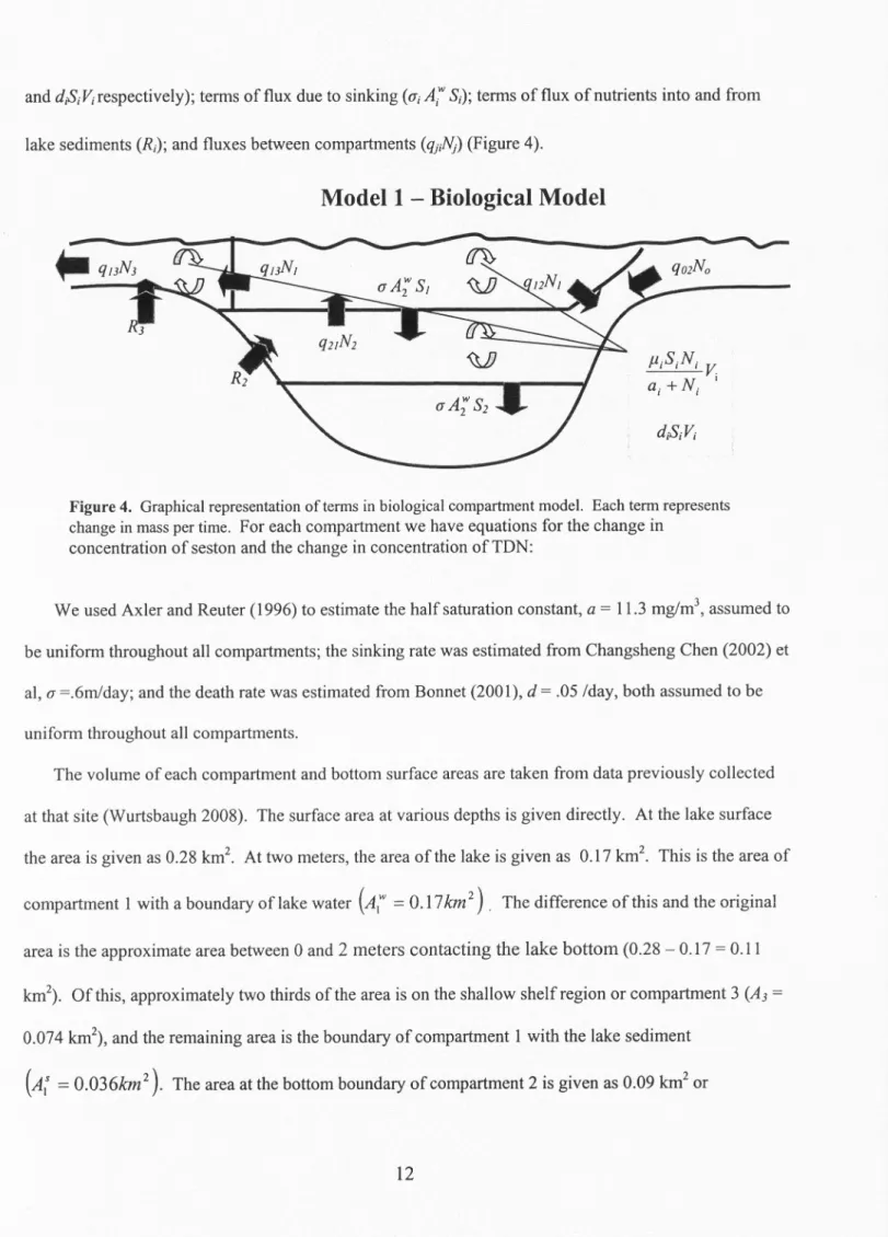
a;+N;

and d;S;V;respectively); terms of flux due to sinking

(a;At

S;); terms of flux of nutrients into and from lake sediments (R;); and fluxes between compartments (q_1;~) (Figure 4).

Model

1 -

Biological Model

µ;S;N; V a;+N; '

Figure 4. Graphical representation of terms in biological compartment model. Each term represents

change in mass per time. For each compartment we have equations for the change in concentration of seston and the change in concentration of TON:

We used Axler and Reuter ( 1996) to estimate the half saturation constant, a = 11.3 mg/m3, assumed to

be uniform throughout all compartments; the sinking rate was estimated from Changsheng Chen (2002) et

al, a =.6m/day; and the death rate was estimated from Bonnet (2001 ), d = .05 /day, both assumed to be

uniform throughout all compartments.

The volume of each compartment and bottom surface areas are taken from data previously collected

at that site (Wurtsbaugh 2008). The surface area at various depths is given directly. At the lake surface

the area is given as 0.28 km2• At two meters, the area of the lake is given as 0.17 km2• This is the area of compartment 1 with a boundary of lake water

(At

=

0.17

km

2) . The difference of this and the original

area is the approximate area between 0 and 2 meters contacting the lake bottom (0.28 - 0.17 = 0.11

km2). Of this, approximately two thirds of the area is on the shallow shelfregion or compartment 3 (A3 =

0.074 km2), and the remaining area is the boundary of compartment 1 with the lake sediment

(A;

=

0.09km

2 ). The difference of

A;

and

A

₁w is the approximate surface area between 2 and 6

meters contacting the lake bottom (

Al

=

0.17 - 0.09

=

0.08 km2) . Compartment 3 has no boundary that does not contact lake sediment.

The volumes are given as the amount of water above a particular depth. Thus to find the volume of any given compartment, the volumes from the depths above are subtracted. The volume above 2 meters is 4.6xl0 5 m3• Of this, approximately one third of the volume is the shallow shelf

(Vi=

l.52x105 m3), and the remainder is compartment 1

(Vi=

3.08xl05 m3). The volume above 6 meters is 9.55x105 m3• The difference of this and the volume at 2 meters gives the volume of the second compartment (V₂

=

4.95x105 m3).

The initial concentrations ofTDN and seston in each compartment are taken from data in 2002 (Baker and Wurtsbaugh 2008). The values for the flows between compartments are calculated daily from the solution of the flow model. The product (R;

=

a; A;b N;') of the velocity of seepage in sediments (a;),

the area of each compartment intersecting the lake bottom ( A;b ), and the concentrations of TDN in the

sediments ( N;') will be determined for each model by minimizing the sum of the squares of the

difference between the measured and predicted values of TDN at the outflow using the MATLAB function,

fminsearch . For a complete list of parameters in each compartment model see Table 2 below. With the above conditions the non-linear system of equations for the first model is solved

numerically for the concentrations of seston and TDN in each compartment, S; and N; respectively (i

=

1,2,3), in terms of time assuming that the compartment volumes remain relatively constant. The system

is put into matrix form and solved using a MATLAB solver.

From this we obtain the concentrations of TDN and seston in each compartment over the given interval. The interval is the amount of time between values of measured TDN at the inflow. Of particular interest is the concentration ofTDN at the outflow (N3), which can be compared with observations.

Symbols

Vi=

3.08x105 m3 V1

=

4.95x105 m3 V3

=

1.52x 10 5 m3

At=0.17km

1

A(

=

0.036km

1

A;= 0.09km

1

A;=

0.08km

2

At

=

0

.

074km

1 a= 11.3 mg/m3 µ1

=

.6 per day µ1

=

.3 per day µ3 = .6 per day d

=

.05 per day a= .6 m/day Description volume of compartment 1 volume of compartment 2 volume of compartment 3

bottom surface area of compartment 1

surface are of compartment 1 with lake sediment bottom surface area of compartment 2

surface area of compartment 2 with lake sediment surface area of compartment

3

with lake sediment half saturation constant

growth rate of Seston in compartment 1 growth rate of Seston in compartment 2 growth rate of Seston in compartment 3 death rate of Seston

sinking velocitv

Table 2. List of variables and constants used in the biological compartment model.

2.5 Flux of TDN in Lake Sediments

We have three terms in the biological model not determined by initial conditions or calculated as variables, namely the terms of the flux of TDN in the sediments (R1, R1, R3). We find R1, R1, and R3 that fit the solution of the biological model to the actual measured values ofTDN at the outflow. This is done by taking the sum of the squares of the errors between the actual and predicted values of TDN on given

Julian days (JD) in 2002.

n

i

=

'

"fJN/R

1

,R

1

,R

3 } -

N

ac

tu

a

/Day = i}J1

i=I

where n is the number of days used.

The minimum of the sum above is found by using the same MATLAB function fminsearch . A function for the solution to the first model is written. The input values are the initial values of the concentration ofTDN and seston for each compartment and a variable vector representing the three sediment terms and the output is the sum above. The matlab function fminsearch finds the optimal choices of R1, R1, and R3 to minimize the sum. The initial inflow and outflow values of TDN were taken

from BTL data in 2002 to find the optimal choices and were then tested against data in 2003 (Baker and Wurtsbaugh 2008).

2.6 Model 2 - TDN Model

The second model is a simplified version of the first model. Analysis of the first model suggested that the

concentration of TON is largely independent of the concentration of seston. Removing the terms of

seston from the system, we have a system of three equations for the concentration of TON in each

compartment based on the flows between compartments and the flux of nutrients in lake sediments. (7) (8) (9)

This system is solved numerically for the concentrations of TON in each compartment in terms of time. The same code is used as the one above with the seston terms removed. The terms of the flux of the concentration of TON in the sediment (R_1, R2, and R3) are recalculated for this new system using the same

method as in section 2.5, that is they are used to fit the data from 2002 and tested against the data in 2003.

2.7 Model 3 - Steady States

The third model is the steady states of the first model with an assumption on the half-saturation constant

(a). The half-saturation constant (a) in the first model was assumed to be much smaller than the

concentration of TON (N;) in each compartment; this changes the nonlinear term of growth between TON

and seston to a linear term:

The biological model turns into a linear system of differential equations. To solve for the steady states we set the changes in concentration of TON and Seston in each compartment to zero. This creates a

homogeneous system of linear equations. This linear system is solved analytically by row reducing and using back substitution to find the steady state solution:

q02No +R2 +R1 q02Noql2 +qo2Noql3 +R2ql2 +R2q13 +Rlql2 q02No +R1 +R2 +R3

N1 = ---,N i= ----'-'---'-'---'-"---'-"---"...c..;;'---"----=--...:...=--, N₃ = --- ( I 0)

q13 q21ql3 ql3

Note that the solution for the steady state of the concentration of seston in each compartment is zero. This is not surprising since the assumption we made removes the dependence of the concentration of seston on the concentration of TON. Also, as mentioned with the first model, the concentration of seston had little effect on the concentration of TON.

Of particular interest is the steady state solution to compartment 3 or the outflow:

where R

=

R 1

+

R2

+

R3 . ( 11) The change in concentration of TON at the outflow is equal to the concentrations of each of the possible sources: the inflow and lake sediments. This is a very basic model in that it is simplified to a simple analytic solution. The sum (R) of the terms for the flux of TON in lake sediments, similar to above, is found to fit the data in 2002 and tested against the data in 2003.

2.8 Model Summary

Each model taken as a whole with the flow model, after determining the entrainment and sedimentation parameters based on outflow and inflow values, takes daily values of the initial velocity of the stream, the temperature of the lake and the inflow, the initial concentration of TON at the inflow and in the lake, and predicts daily values of the concentration of TON at the outflow. The results of each of the three models are presented below.

3 Results -

Biological Model, TDN Model, and Steady States Model

For each of the three models, the terms of flux of TON in the lake sediments (R1, R2, R3) were used to fit the predicted values of TON with the actual values of TON from data in 2002. Each of the three models was then tested against data in 2003. The results for each model including the terms of flux in lake sediments and qualitative analysis are summarized below (Figure 5 and Table 3).

Results of Biological Model 400 'E oi E 300 z 0

l-o

200 C g ~ ~ 100 (.) C 0 (_)

Model 1 - Biological Model

180 200 220 240 260 Julian Days in 2002 400 'E oi E 300 z 0

l-o

200 C g ~ ~ 100 (.) C 0 (_)

Model 1 - Biological Model

.

_...

.

...

200 210 220 230

Julian Days in 2003

Results of Biological Model - Seston

C 0 200 gj 150 (/) 0 5 100 :;::; ~ c <I) g 50 0 (_)

Measured vs Actual Seston 2002

?40 160 180 200 220 240 260 Julian Days in 2002 Figure Sa. 200 C

s

~ 150 (/) 0

5

100 :;::; ~ c <I) g 50 0 (_)

Measured vs Actual Seston 2003

200 210 220 230 Julian Days in 2003 Results of TDN Model 400

1:

ai E 300 z 0

l-o

200 C 0 :;:::: ~ ~ 100 u C 0

Model 2 - TON Model

.

.~.

V • • • .•~

...

_{. .}

400

1:

ai E 300 z 0

l-o

200 C 0 :;::; ~ ~ 100 (.) C 0 0 0 ?40 160 1ao 200 220 240 260 ?9o Figure Sb.

Model 2 - TON Model

...___

..

_.

_.

•

.

...

200 210 220 230 Julian Days in 2003 240 240 240

400 1: C) E 300 z D t-~ 200 0 :;:; ~ ~ 100 u 5 (.)

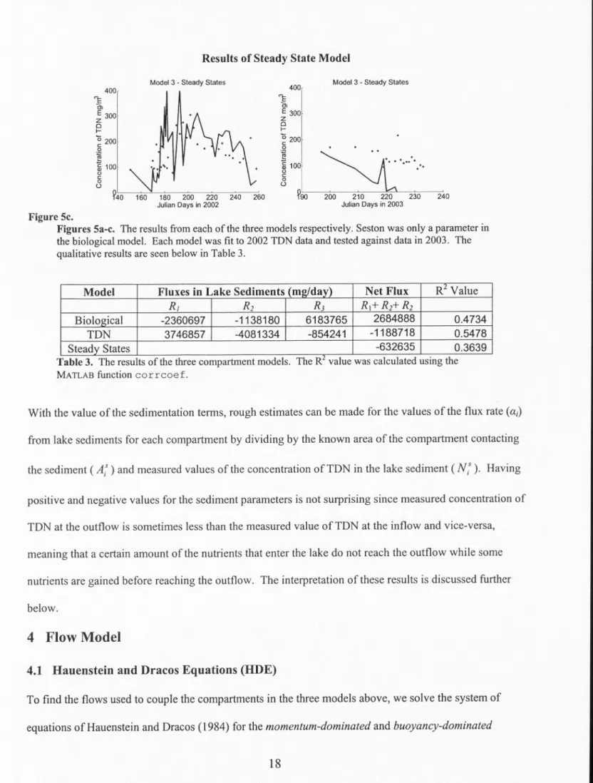
Results of Steady State Model

Model 3 -Steady States

400 1: C) E 300 z 0 t-~ 200 0 ~ ~ 100 u C 0 (.)

Model 3 - Steady States

.··

~40 160 180 200 220 240 260 Julian Days in 2002 ~90 200 210 220 230 240 Julian Days in 2003 Figure 5c.

Figures 5a-c. The results from each of the three models respectively. Seston was only a parameter in the biological model. Each model was fit to 2002 TDN data and tested against data in 2003. The qualitative results are seen below in Table 3.

Model Fluxes in Lake Sediments (m2/day) Net Flux R2 Value

R, R1 R3 R1+ R1+ R1

Biological -2360697 -1138180 6183765 2684888 0.4734

TDN 3746857 -4081334 -854241 -1188718 0.5478

Steady States -632635 0.3639

l

Table 3. The results of the three compartment models. The R value was calculated usmg the MATLAB function corrcoef.

With the value of the sedimentation terms, rough estimates can be made for the values of the flux rate (a;)

from lake sediments for each compartment by dividing by the known area of the compartment contacting

the sediment (A:) and measured values of the concentration of TDN in the lake sediment ( N: ). Having positive and negative values for the sediment parameters is not surprising since measured concentration of

TDN at the outflow is sometimes less than the measured value of TDN at the inflow and vice-versa,

meaning that a certain amount of the nutrients that enter the lake do not reach the outflow while some

nutrients are gained before reaching the outflow. The interpretation of these results is discussed further

below.

4 Flow Model

4.1 Hauenstein and Dracos Equations (HDE)

To find the flows used to couple the compartments in the three models above, we solve the system of

regions of the inflow into the lake. The flow rates between the remaining compartments are found by assuming conservation of volume.

Where a density difference exists between the inflow and lake water a density current will be generated by the inflow (Fleenor 2000). The density of water increases as temperature decreases (until about 4°C at which point liquid H20 has maximum density). Solar input warms surface water causing a density difference between the current from the inflow and the lake water; due to the higher density and the slope of the lake bed, the colder inflow plunges beneath the warmer lake water until it reaches a neutral buoyancy at which point it inserts into the lake (see Figure 6 below). Hauenstein and Dracos applied separate integral models to each region based on the steady state mass and momentum balances of the Boussinesq (NSB) approximation (Hauenstein 1984).

The Plunge

S=O

Insertion Point x1

Figure 6. Diagram of the momentum and buoyancy-dominated regions.

For each region, we assume the density current has the following characteristics: the inflow stream is of fixed height (h0 ) and breadth (b0 ), with initial velocity (u0 ), the lake bed has a fixed slope (S) from the

inflow; the lake water is of density (p), the current is of density (pc) where 1':J..p is the difference in density; with the gravity constant (g), and insertion point (x1). The horizontal entrainment (ah) is defined by a

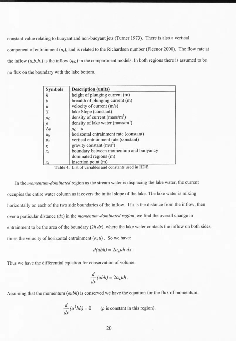
constant value relating to buoyant and non-buoyant jets (Turner 1973). There is also a vertical

component of entrainment (a,), and is related to the Richardson number (Fleenor 2000). The flow rate at the inflow (u0b0h0 ) is the inflow (q02) in the compartment models. In both regions there is assumed to be

no flux on the boundary with the lake bottom.

Symbols Description (units)

h height of plunging current (m)

b breadth of plunging current (m)

u velocity of current (mis)

s

lake Slope (constant)

Pc density of current (mass/m3)

p density of lake water (mass/m3)

tip Pc-p

ah horizontal entrainment rate (constant)

°'2 vertical entrainment rate ( constant) g gravity constant (m/s2)

x,

boundary between momentum and buoyancy dominated regions (m)

x,

insertion point (m)

Table 4. List of variables and constants used in HDE.

In the momentum-dominated region as the stream water is displacing the lake water, the current occupies the entire water column as it covers the initial slope of the lake. The lake water is mixing horizontally on each of the two side boundaries of the inflow. If xis the distance from the inflow, then over a particular distance (dx) in the momentum-dominated region, we find the overall change in

entrainment to be the area of the boundary (2h dx), where the lake water contacts the inflow on both sides, times the velocity of horizontal entrainment (ah u) . So we have:

d(ubh)

=

2ahuh

dx.

Thus we have the differential equation for conservation of volume:

d

-(ubh)

=

2ahuh.

dx

Assuming that the momentum (pubh) is conserved we have the equation for the flux of momentum: (p is constant in this region).

The lake bed slope (S) is assumed to change linearly which gives the equation for the height of the current:

h

=

h

0

+

Sx.

We thus have the equations for the momentum-dominated region as defined by Hauenstein and Dracos (1984): conservation of volume x-momentum geometric condition d

-(ubh)

=

2ahuh

dx

(12) (13) (14) The equations for the buoyancy-dominated region as given by Hauenstein an Dracos (1984) are:

conservation of volume

x-momentum

y-momentum

conservation of buoyancy

d

-(ubh)

=

2ahuh +

la,ub

dx

!!_(u

1

bh)

=

_!_!!_(,1p gbh

1)-

,1p gbhS

dx

2dx

p

p

d

1

,1p

2

-(uvbh)

=

--

gh

dx 2 p

d (,1p

)

dx Pgubh

=0

(15) (16) (17) (18)

Here the ambient lake water is entrained from both sides of the inflow as well as from a single boundary above. The vertical boundary over a distance (d.x), where the lake water is above the inflow, is found by the surface area of the upper boundary of the current (b dx) times the velocity of vertical entrainment (a, u). The horizontal entrainment from each side and the vertical entrainment from above give us the above differential equation for volume. The momentum is no longer considered constant. Density differences in both regions can be found using the conservation of buoyancy.

Equations 12-14 are solved analytically for the velocity (u,), the breadth (b,), and the height (h,) at the boundary between the two regions given empirical values for u0 , b0 , h0 , the slope (S), the constant

entrainment value (ah), and the boundary between the two regions (x,) . The system of equations for the buoyancy- dominated region are solved numerically for the velocity (u1), the breadth (b1), and the height

(h1) at the insertion point (x1) given the values of velocity (u,), breadth (b,), and (h,) at the boundary between the two regions, entrainment constant value ( az), values of

lake density

(p)

and the difference

in density

(tip) at the boundary, the insertion point (x1), and certain geometric assumptions on h, which

will be outlined below. The sum of the inflow rate (q02) and the entrainment rate (q12) in the compartment

model is given by u1b1h1.

4.2 Bull Trout Lake-Field Study

In order to test the parameters of the density current included in the flow model, namely the breadth (b), height (h), and velocity (u) of the current, a field study was conducted at Bull Trout Lake (BTL) from June 17 to June 23, 2009. BTL is one of many lakes in the Sawtooth Mountain range located in Central Idaho (Figure 7).

Figure 7. Image of Bull Trout Lake in Central Idaho near Stanley, Idaho.

<http://images.google.com/imgres?imgurl=http ://picturesofcascade.corn/1arge7/

These lakes reach their peak inflow around mid-June. During peak flow, as part of an extensive study conducted by Montana State and Utah State Universities, rhodamine WT, a fluorescent tracer, was injected into the lake about 50m upstream continuously from June 21st to June 23rd (Figure 8).

- _....:. -=-~- :;-:--~ ·~. ----.. ·-,~.•·••:; ... :..:.--i...• .

. --::

Figure 8. Image ofrhodamine being dripped into Bull Trout Lake. Also notice the delta that extends about 25 meters out from the initial inflow. Picture courtesy of Wurtsbaugh et al (Wurstbaugh 2008).

Using a submersible fluorometer, CYCLOPS (Turner Designs, Inc.) voltage was measured to determine rhodamine concentrations throughout the lake. In order to measure the breadth and depth of the plunge into the lake near the inflow, a fence post was placed about 3 meters from the end of the delta that extends about 23 meters into BTL. A rope was connected between the post and the row boat, and the rope made taut so as to stay a consistent distance from the inflow. One person rowed the boat in circular arcs around the inflow while a second person placed the fluorometer at a specific depth and continuously recorded the voltage throughout each arc (Figure 5). Arcs were completed at distances of 15, 30, and 65m at depths of

. • . ' .t. •~~ ----· 44'17'!:0 64. N 115'15'C9 43'W Image .fl 2008 OlgltalGlobe ~, 2008 To1o Alla• eie·, 896211 ,-Google· Eye alt 7808 It

Figure 9. Arcs were completed around the inflow using a fluorometer to measure the breadth of the density current. image © 2008 DigitalGlobe, © 2008 Tele Atlas

The breadth (b) was measured by taking the GPS coordinates for the boundaries of high voltage and

estimating the length of the arc between them. Depending on the estimated distance to the insertion point,

the breadth can vary; the value used for solving the equations is 70 meters (Figure I 0).

lrn•lilo ti:) 2008 Cllillla!Qloba

1Eyaa1t 772511

Figure 10. Arcs were completed near the inflow to show the path of the density current and measure its breadth. Red dots indicate peak concentrations of rhodamine, and green dots indicate high

concentrations of rhodamine. image © 2008 DigitalGlobe, © 2008 Tele Atlas

In order to estimate the height of the density current, an anchor was used to steady the boat, and the fluorometer was lowered to get a vertical map of the rhodamine concentration in the lake. The height of the density current is estimated by looking at peaks in concentration. The data from the vertical transect were plotted against the depth of the lake (Figure 11). When completing a vertical transect, the

fluorometer contacts the lake bottom, and sediment is disturbed creating outlying concentrations not due to rhodamine. These concentrations are ignored in the measurement. Depending on the insertion point, the height of the peak concentration may vary; at the estimated insertion point the value of h was measured to be 2 meters. DepWCorcerlration Profile

o

---~

.$ ,5 6 0. ., 0 10

....

.

-

...

.

-...

...

..

1

_to

100 120 140 160 180 200 220 240 Corcermition (Vols)

Figure 11. A vertical transect was taken to measure the height of the density current. The second peak represents the fluorometer displacing lake sediment as it contacts the lake bottom and is ignored in the height measurement.

As mentioned with the breadth and the height, the location of the insertion point (x1) of the density

current is critical to the flow model. The density current depends on the density of the water in the current which in tum depends on the temperature of the water. As warmer lake water is entrained into the

colder density current, the temperature of the current rises. At the same time, the lake water grows colder

as the current plunges deeper. When the temperature of the current matches the temperature of the lake, the density will equalize and the current will insert into the lake. The depth at which this occurs is

assumed to be the thermocline of the lake. Throughout the lake, vertical temperature transects were taken to estimate the depth of the thermocline (Figure 12).

Vertical Temperature Transcript Afternoon Jun 21

o

~---~

•

---..---_§, 6 • .c a. Q) 8 Cl 10 12 • •

•

7.5 8.5 9.5 Temperature -°C Thermocline

Figure 12. A vertical transect of the lake temperature on June 21, 2009. The thermocline is measured at Sm.

Measurements of the thermocline vary at different points in the lake and at different times during the day.

For instance, in the afternoon near the inflow (within 100 m), the thermocline was measured near the

surface to be 1.5 to 2 meters. Early in the morning near the inflow (within 100 m), the thermocline was

measured deeper to be 5 to 6 meters (Figure 12 above). In the lake models, the middle layer or

compartment is defined to encompass the upper and lower bounds for the measured values of the insertion

point.

With the depth of the thermocline measured and the assumption that the plunge inserts near the

thermocline the point of insertion (x1) is measured using lake morphometry (Figure 13).

•

BTL Lake Morpho~:~z;

---

·

Insertion Point

/

'

\

_______ ___,/ i

Outfl~

_,

//

---:-

_/

_

_

11

30

1

1l1

/·

~

·

/ N -

I

l 6m 0 • 16m I

I

g u \

\_

/

Inflow

--\ _{. ---....__,../} ,/ ·,,., 2m (. ', Shallow Sitelf // '"--- ----·--- ---

--N

810m

Figure 13. Contour map of BTL. The lake flow from south to north, has a large shallow shelf along the northwestern side. of the lake, a delta that runs about 23 meters into the lake, and a maximum depth of about 16 meters.

The estimated depth of the bottom of the middle compartment (6m) was located on the map, and the distance from the inflow to the first marker of 6m in the direction of the density current was calculated. The insertion point was measured to be 30 meters.

The boundary between the momentum-dominated and buoyancy-dominated regions (x1} was

determined by observing the flow of rhodamine into the lake. At BTL, from the inflow extends a small delta about 23 meters into the lake (Figure 8). During high flow in the summer, the water flows over this delta before reaching the initial slope of the lake bed. The density current was observed to plunge very near the end of the delta at the first major change in the slope of the lake. From this observation, the boundary between the two regions was determined to be 23 meters.

The height of the current over the delta was relatively flat and was measured to be a constant h = 0.2 m for 0 :'.S x :'.S 23. The slope (S) of the lake is 0 over the delta. The slope of the lake over the buoyancy-dominated region (0.25) was measured by taking the depth at the insertion point and the depth at the end of the delta. The initial breadth of the current near the inflow at the beginning of the delta was measured to be 5 meters. The velocity of the density current (u) was measured at the inflow using a flow meter. Near the inflow at the location of the plunge, measurements could only be taken from the boat. Due to the unsteadiness of the boat an accurate measurement of the velocity at different depths was not possible. Thus the velocity of the current at the insertion point (u1) could not be measured directly. It was

observed, however, rhodamine had crossed the entire length of the lake within 24 hours of release. The length of the lake was measured to be approximately 810 meters, and dividing this by one day we have:

810m

8xl0

4

cm

=---lday

8.64xl 0

4

sec

8cm

---

~

.93cmlsec.

8.64sec

This is the approximate minimum velocity required for the current to traverse the entire lake in one day and is a rough estimate of the minimum velocity at the insertion point (u1). This was used as an estimate

of the value of the velocity at the insertion point (u1). Values used in calculations are summarized in the table below and shown in the figure below.

Symbols Description

h0 = 2 cm height of the current over the delta (0 :'S x :'S x1)

b0

=

5 m initial breadth of density current S =0 lake Slope over delta (0 :'S x :'S x1) S =.25 lake Slope from delta (x1 :'S x :'S x1)

x1 =23 m boundary between momentum and buoyancy

x1 = 30 m dominated regions

b1 = 70 m insertion point determined by thermocline

h1 =2m breadth of current at insertion point

u1 = .93cm!s height of current at insertion point velocity of current at insertion point

Table 5. Measured values for HDE parameters and boundary conditions at BTL.

The Plunge

S=O

Figure 14. A graphical depiction of the plunge into Bull Trout Lake. Measurements were taken from

field data collected in the study in 2008.

The initial velocity (u0 ) of the inflow is determined from daily discharge data taken near the inflow

(Arp 2006). The initial velocity is found by taking the discharge (m3/sec) and dividing by the initial breadth (b0 ) and the initial height (h0 ). The initial density of the current (pc,0 ) is determined from temperature data at the inflow (Wurtsbaugh 2008). Values of water density based on temperature were taken from a table of values for distilled water (Walker 1998). From these values, a quadratic formula was fit to the data using a build in MATLAB fitting tool:

Using this relation, the lake and current densities were calculated. The initial density differential used in the flow model (equations 16-18 (!:!..p/p)0 ) was found by taking the difference of the initial densities of the

lake and inflow and dividing by the initial density of the lake taken at the bottom of compartment I. The differential in density was then calculated as a variable in the model.

4.3 Solution to Hauenstein and Dracos Equations for BTL

4.3.1 Solution in Momentum-Dominated Region

With the initial values of h0 , b0 , S, the plunge point (x1), and the initial velocity (u0 ) determined from

discharge data, the system of equations for the momentum-dominated region is solved analytically. In the geometric condition (Equation 14), the slope (S) is zero over the delta, so we have the height as a

constant:

h = h0 = 0.2m. (8)

Using equations 13 and 14, we integrate both sides with respect to x to find:

The height h

=

h0 divides out. We then solve this for b to find:

b

=

u;b

0 2 •

u

(9)

This is substituted into the equation for the conservation of volume (12):

Using separation of variables, we integrate (12) to find:

Substituting this back into equation (13) to solve for b, we have the solution to the system of equations in the momentum-dominated region:

h

=

0.2m (14)

(19)

u=

(20)

The flow rate (m3/s) oflake water being entrained in the momentum-dominated region (Qmd) can be found by subtracting the initial flow rate from the flow rate at the plunge point:

The value Qmd will later be added to the rate of entrainment in the buoyancy-dominated region (Qbd) to determine flow between compartment 1 and 2 (q12) in the compartment models.

The values of u,. b,,and h1 at the plunge point (x,) are also initial conditions for the

buoyancy-dominated region. The value of the entrainment rates ah and a2 are determined given the measured values

of u1, b1, and h1 at the insertion point.

The variable of density (!1plp) in the momentum-dominated region is determined from the conservation of buoyancy (18). Integrating both sides and solving for 11p/p we have:

d (ilp ) ilp

-

--gubh

=0

•

-ub=C.

dx

p

p

The constants g and h are independent of x and divide out of the equation. With the initial conditions at x = 0 we solve for the constant C and determine the variable of density:

From this we can find the variable of density at the plunge point ((/).plp)1, which is an initial condition for the buoyancy-dominated region.

With the values at the plunge point (x,) of the slope (S), the height (h,), the breadth (b,), the velocity

(u,) and the variable of density ((t,,.p/p), we solve the system of equations 15-18 in the

buoyancy-dominated region. In the four equations, we have five variables: u, v, b, h, and t,,.p. The vertical velocity

( v) is found only in equation 1 7. The other variables are therefore independent of v, so equation 17 is not needed to determine the other parameters, and the system reduces to equations 15, 16, and 18.

That still leaves four variables with just three equations, so to solve the system, we assume that the height of the current grows in a smooth manner from 20cm on the delta (x,) to 2m at the insertion point

C

h(x)

= -'

+

C_{2 ,} where C, and C2 are constants.

X

The constants C, and C2 are determined by these values, that is the height and distance at the plunge point

(h, = 0.2m and x, = 23m) and the height and distance at the insertion point (h1 = 2m and x1

=

30m).

We have:

Plugging in the values and solving for C2 we have:

Plugging this into the equation at the insertion point we have:

From this we find:

c,

c

2 =.2--~1.n.

23

We thus have the estimated height of the current in the buoyancy-dominated region:

h(x)

=

-177.51

+

7.92.

X

With this geometric assumption, the non-linear system of differential equations for the buoyancy-dominated region (equations 15, 16, and 18) is solved numerically using the built in MATLAB differential equation solver ode 15 s. Differentials in each equation are expanded using the product rule to obtain:

du

db

dh

-bh+u-h

+ub-

=

2ahuh+lazub

dx

dx

dx

d ( ilp)

ilp du

ilp db

ilp

dh

-

--

gubh+--gbh+-u-gh+-gub-=0

dxp

pdx

p

dx

p

dx

The system is put into matrix form for the solver to run:

du

-bh

uh

0

_dx

2ahuh +a

z

ub

2ubh

u2h

_.!:__

ilp gh2

gbh

2

_db

ilp gbhh'-u

2

_{bh'- ilp gbhS}

---

=

2

p

2

dx

p

p

ilp gbh

ilp guh

_gubh

!(~)

- ilp gubh'

p

p

p

Solving these equations with known

ah

and O.z, we obtain the velocity (u), breadth (b), and variable of

density (!).pip) over the buoyancy-dominated region (x, :S x :S x1). The flow rate (m3/s) of lake water being

entrained in the buoyancy-dominated region (QM) can be found by subtracting the flow rate at the plunge point from the flow rate at the insertion point:

The sum of the two entrainment rates (Qmd + Q6d

=

q12) is the flow rate between compartment 1 and compartment 2 of the three lake models.

Known values for ah and az and initial conditions for the velocity (u0 ), breadth (b0 ), and height (h0 )

can be used to predict the values at the insertion point (u1, b1, and h1 respectively). Instead, we have

4.4 Eigenvalue Problem for

ah

and

az

The measurements found at the insertion point (x, = 30m) of the breadth (b₁ = 70m), and the velocity

(u1 = .93cm/s) can now be used to determine the values for ah and az, that is, we solve the problem:

u(ah,az) - U1

=

0

b(ah,az) - b1 = 0

Put simply we find ah and az, that fit the solution of the flow model to the actual measured values of the breadth and the velocity. We therefore have two free variables and two conditions to solve making this an eigenvalue problem. To find ah, and az we minimize the sum of the squares of the errors between the actual and measured values for b and u at the insertion point.

E(ah,az)

=

(u(ah,az) - u,)2

+

(b(ah,az) - b,)2.

This is done by using the built-in MATLAB function fminsearch . A function for the solution to

equations 12-15, 17 and 18 is written including the momentum and buoyancy-dominated regions. The

input values for fmin search are the function for the solution with initial values at the inflow and a variable representing the two entrainment rates and the output is the error above. The MATLAB function

fmins ea rch then finds the optimal choices of ah and az to minimize the error. The basic code is given below (Figure 15). The measurements above were taken near peak flow in late June. The initial values were taken from June and July in 2002 (Table 6). Taking the average of the calculated a/sand

a

/

s

,

we have ah

=

.0095 and az

=

.010 I. These rates are much smaller than those found in literature values; ah

=

.1 as defined by Turner (1973). With these two entrainment rates, the solution to the flow model can be found to give the flow rate at the insertion point (q21

=

u,b1h1) and the flow rate of entrainment (q 12

=

Qmd

+

[[alphah alphaz),minerror,ef] = fminsearch(@(x) HDE([initial values),x), [gue ss))

function

error= HDE([initial values],x)

[X Y) = odelSs (b, [interval), [Values at Plunge Point), A);

u = Y(end,1)

b

= Y(end,2)

error= (u

-

.0093)1'2

+

(b - 70)1'2

Figure 15. Code for finding ah,az that minimize the error between the predicted values of u1 and b1

from the model and the actual values measured from field data (u1 = .0093m/s and b1 = 70m). Initial

values can be found in figure 9. A guess is made for the values of ah and O.z as a starting point for the matlab function. An exit flag (ef) is given to indicate if the MATLAB function found a minimum or reached its set limit of calculations.

JD 2002 Input Values Results _E(ah,az)

Uo (m/s) LTemp (OC) STemp (OC) _{0.h az}

151 0.10378 5.07375 5. 39667 0.009095 0.010532 l.44E-05

171 1. 30099 8.04659 5.96333 0.009219 0.010415 0.010154

176 0.752 8.10197 6.105 0.009243 0.010412 0.002952 214 0.497 12.90089 7.10667 0. 010072 0.010089 0.001086

Table 6. Results of solving for ah and az, where JD is Julian day, L Temp is the temperature of the lake, STemp is the temperature of the inflow, and Eis the total entrainment rate. Input data taken from discharge data in 2002. Alphas are found using the built in MATLAB function fminsearch .

4.5 Flow Model Summary

In solving the Hauenstein and Dracos Equations (1984 ), flow rates of entrainment and flow rates at the

insertion point were found using physical data taken at the field study in 2008. As mentioned above in determining the breadth and the depth of the plunge, the insertion point is critical. Several methods were used to calculate the insertion point. The insertion point was left free in the flow model and was

approximated by placing tolerances on the temperature and velocity and finding distance at which the model reached these values. Small changes of the insertion point in the model yielded dramatic differences in the breadth of the flow due to the rapid growth of the breadth from the inflow. However, when coupling the breadth with the velocity, which was decreasing, the overall flow at the insertion point was not as sensitive to changes in the insertion point. For example, insertion point changes of ±5 meters altered flow rates by approximately 0.05%. Therefore, the compartment models for TDN are not sensitive to minor changes in the insertion point.