Large-Scale Spatial Join Query Processing in Cloud
Simin You
Dept. of Computer ScienceCUNY Graduate Center New York, NY, USA
Jianting Zhang
Department of Computer ScienceThe City College of New York New York, NY, USA [email protected].edu
Le Gruenwald Dept. of Computer Science The University of Oklahoma
Norman, OK, USA [email protected] Abstract— The rapidly increasing amount of location data
available in many applications has made it desirable to process their large-scale spatial queries in Cloud for performance and scalability. We report our designs and implementations of two prototype systems that are ready for Cloud deployments: SpatialSpark based on Apache Spark and ISP-MC based on Cloudera Impala. Both systems support indexed spatial joins based on point-in-polygon test and point-to-polyline distance computation. Experiments on the pickup locations of ~170 million taxi trips in New York City and ~10 million global species occurrences records have demonstrated both efficiency and scalability using Amazon EC2 clusters.
Keywords—Spatial Join, Spark, Impala, Cloud Computing I. INTRODUCTION
GPS devices and smartphones have generated huge amount of location data. Very often point location data need to be joined with urban infrastructure data, such as road networks and administrative zones, to better understand human mobility patterns and, subsequently, improve urban planning, traffic control and infrastructure maintenance. As an example, more than 13,000 taxicabs in New York City (NYC) have been generating half a million taxi trips a day, each with pick-up and drop-off locations and timestamps. This amounts to nearly 170 million taxi trips severing more than 300 million passengers every year. Many of the scientific datasets also have a geospatial component and need to align with global and regional ecological and administrative zones to facilitate scientific investigation and discovery. For example, the Global Biodiversity Information Facility (GBIF1) has accumulated more than 400 million species occurrence records and many of them are associated with a (latitude, longitude) pair. It is essential to map the occurrence records to various ecological regions to understand the biodiversity patterns and make conservation plans. All these applications require spatial join query processing, a well-defined problem in spatial database research [1] and its solutions have been provided by major commercial and open source spatial databases as well as Geographical Information Systems (GIS). However, the amounts of spatial data in these applications (e.g., in the order of tens to hundreds of millions of data items) well exceed the processing capabilities of traditional disk-resident systems running on single computing nodes and thus require new systems to reduce processing times from days or hours to minutes or even seconds in order to be practically useful for researchers and decision makers [2].
1http://data.gbif.org/
Existing works on processing large-scale spatial join query processing mainly fall into two categories: a) improving single-node efficiency by exploiting the massive data-parallel computing power of hardware accelerators, such as Graphics Processing Units (GPUs) that are capable of general computing, and b) exploiting scalability provided by Hadoop/MapReduce based systems. Here MapReduce is referred to both as a computing model and as a component in Hadoop (together with the Hadoop Distributed File System– HDFS). Our previous work on GPU-based spatial joins [2,3] have demonstrated that it is quite possible to achieve orders of magnitude of performance improvements by re-designing and re-implementing spatial joins from scratch, which requires significant amounts of efforts. Despite of the fact that Cloud computing vendors such as Amazon EC2 have provided GPU-instances2, which makes it possible to scale the single-node implementations to Cloud computing resources, the technique is less mature from an end-user perspective with respect to easiness of deployment, robustness of operation and cost-effectiveness of Cloud resource utilization. In contrast, alternative techniques, such as SpatialHadoop [4] and HadoopGIS [5], aim at utilizing existing mature Cloud computing techniques and tools (Hadoop/MapReduce in particular) and adapt traditional serial designs and implementations for easy parallelization and Cloud deployment. While a more detailed discussion of such techniques is provided in Section 2, we would like to argue that many of them suffer from the combined platform and implementation related inefficiencies which significantly limit their capabilities to process spatial joins on large-scale data in Cloud efficiently.
In this study, we report our designs and implementations of large-scale spatial join query processing on two leading in-memory Big Data systems, namely Apache Spark3 and Cloudera Impala4, and compare their performance using real world large-scale datasets. Spark is considered as the succession of the batch-oriented Hadoop/MapReduce system by leveraging efficient in-memory computation for fast large-scale data processing. However, to the best of our knowledge, Spark has not been used for spatial join query processing. While Impala is designed as a high performance SQL query engine to process relational queries in-memory for end users, in this study, we have successfully extended Impala to process spatial joins on multi-core CPUs.
2 http://aws.amazon.com/about-aws/whats-new/2010/11/15/announcing-cluster-gpu-instances-for-amazon-ec2/ 3 https://spark.apache.org/ 4 http://www.cloudera.com/content/cloudera/en/products-and-services/cdh/impala.html
Our technical contributions in this study can be summarized as follows. First, we have implemented two spatial join algorithms, one is based on point-in-polygon test5 and one is based on point-to-polyline distance, on both Spark and Impala that can be easily deployed in Clouds. Second, we have performed extensive experiments on the implementations using real world large-scale datasets on a 10-node Amazon EC2 cluster and reported their performance. Third, based on our experiments, we have provided a preliminary analysis of the advantages and disadvantages on extending Spark and Impala for large-scale spatial join query processing which can be valuable for developing Cloud-based big spatial data systems in the future.
The rest of the paper is arranged as follows. Section 2 introduces background, motivation and related work. Section 3 and Section 4 present the designs and implementations of our SpatialSpark (based on Spark) and ISP-MC (based on Impala) prototypes for spatial joins, respectively. Section 5 is experiments and performance evaluations of the two systems. Section 6 compares SpatialSpark and ISP-MC and discusses alternative options based on our experiences gained from this study. Finally, Section 7 is the conclusion and future work directions.
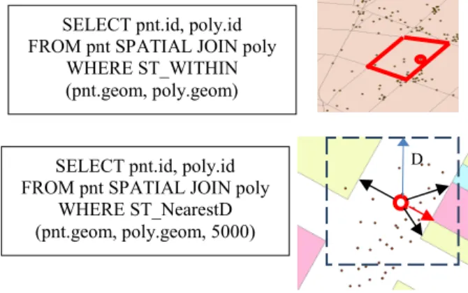
II. BACKGROUND, MOTIVATION AND RELATED WORK Given two spatial datasets and , the result of a spatial join over and can be defined as the following:
, | , , , ,
where is a spatial predicate for the relationship of two spatial objects. Examples of spatial predicates include point-to-polyline distance computation, i.e., searching for nearest polyline within distance D (termed as NearestD), and point-in-polygon test (termed as Within). A naïve implementation of a spatial join is to first pair all objects from and (cross join) and output pairs that satisfy the spatial predicate in the spatial join (selection). The naïve approach incurs a total complexity of · which makes it very inefficient. To speed up spatial join query processing, either the left side table, the right side table or both can be indexed. Typically the process of pairing spatial objects using Minimum Bounding Box (MBB) approximation (with or without using indices) is called spatial filtering, and the process of evaluating the spatial relationships between the paired spatial objects is called spatial refinement [1]. Spatial filtering is tightly related to spatial indexing and query optimization which is more data intensive due to the MBB approximation. On the other hand, spatial refinement relies on efficient computational geometry algorithms. This is because testing spatial relationships between two spatial objects can be computationally intensive, especially when both spatial objects have large numbers of vertices and complex internal structures. We refer to [1] for a survey on spatial joins.
As most of the existing algorithms and systems for spatial data processing are serial [1], it is quite challenging to adapt them to modern parallel hardware and distributed systems. While many parallel and distributed computing models,
5 http://en.wikipedia.org/wiki/Point_in_polygon
programming tools and runtime systems such as OpenMP6, Intel TBB7 , Bulk Synchronous Parallel (BSP8) and MPI9 have been introduced in the past, their impacts on data management community is relatively insignificant when compared with MapReduce [6] and its Hadoop open source implementation10. By requiring developers to provide only a map function and a
reduce function in a job, Hadoop/MapReduce is able to
automatically parallelize the job and distribute map and reduce
tasks to distributed computing nodes with an implicit shuffle
phase. This largely eliminates the needs of worrying about low level data communication and concurrency control, which are non-trivial and error-prone for data management software developers. The initial success of Hadoop based applications (e.g., word count and page rank) have motivated both industry and academia to research on how to formulate their domain-specific problems as Map/Reduce tasks in order to use Hadoop for easy parallelization and distribution. SpatialHadoop [4], HadoopGIS [5] and ESRI Spatial Framework for Hadoop11 are three open source systems that are designed to process large-scale spatial data on Hadoop. While they differ significantly with respect to functionality and implementations, they all spatially partition spatial data to apply the MapReduce computing model. Although cross joins are embarrassingly parallelizable and fit the MapReduce framework well, they are efficient at neither the partition level nor the data item level. As such, both HadoopGIS and SpatialHadoop support indexed spatial joins on partitions to speed up pair-wise cross joins.
Fig. 1 Spatial Join Query Examples
In SpatialHadoop, both sides in a spatial join are partitioned and spatial join is implemented as a map-only job. By providing a custom FileInputFormat based on the spatial layouts of the partitions of both sides, SpatialHadoop pairs up spatially overlapping partitions, which are subsequently assigned to map tasks for parallel and distributed execution. SpatialHadoop elegantly utilizes custom FileInputFormat and implements spatial filtering as a preprocessing step in a map
job that is natively supported by Hadoop. In contrast, HadoopGIS first reorders the joining datasets of both sides so that data items belong to the same partition are stored in the
6http://openmp.org/wp/ 7 https://www.threadingbuildingblocks.org/ 8 http://en.wikipedia.org/wiki/Bulk_synchronous_parallel 9http://en.wikipedia.org/wiki/Message_Passing_Interface 10 http://hadoop.apache.org/ 11 http://esri.github.io/gis-tools-for-hadoop/
SELECT pnt.id, poly.id FROM pnt SPATIAL JOIN poly
WHERE ST_WITHIN (pnt.geom, poly.geom)
D SELECT pnt.id, poly.id
FROM pnt SPATIAL JOIN poly WHERE ST_NearestD (pnt.geom, poly.geom, 5000)
same HDFS blocks. By using the partitions as keys and data items as values, data items in both sides that belong to same partitions are paired at the partition level after the map and
shuffle stages. In the reduce stage, a partition pair is assigned as a reduce task and nested loop joins or indexed joins can be applied to the data items within the partition. While SpatialHadoop uses binary representation in both memory and disk and is capable of accessing data items randomly, HadoopGIS adopts the Hadoop streaming technique which requires all intermediate results to be represented as text where accesses are strictly sequential. Despite being less efficient as both data movement and parsing text are expensive on modern hardware, HadoopGIS allows running programs that are not written in Java as map or reduce tasks which is convenient. In fact, HadoopGIS uses the open source libspatialindex12 for spatial indexing/filtering and GEOS13 for spatial refinement, both are written in C/C++.
Existing Cloud computing applications based on Hadoop have been praised for high scalability but criticized for low efficiency [7]. Indeed, outputting intermediate results to disks, although advantageous for supporting fault-tolerance, incurs excessive disk I/Os which are getting significantly expensive when compared with floating point computation on modern hardware [8]. As computers are increasingly equipped with large memory capacities, in-memory big data systems designed for high performance, such as Apache Spark based on Scala and Cloudera Impala based on C++ (backend), have been gaining popularities since their inceptions. While there are a few previous works on using Spark and Impala for spatial indexing and retrieval (e.g. [9]), we are not aware of existing works on large-scale spatial join query processing on the new generation big data systems in Cloud. We note that, however, it is not our intension to compare our work with spatial data processing systems based on Hadoop directly as they are designed for different types of applications (e.g., interactive vs. batch), require different hardware resources (e.g., large memory capacities) and support different features (e.g., fault-tolerance). Our goals are to understand the potential performance of modern hardware for spatial join query processing at large scale and to identify architectural advantages and limitations of Spark and Impala for spatial data processing in Cloud.
III. SPATIALSPARK: IMPLEMENTING SPATIAL JOINS ON SPARK Spark is built on the notion of RDD (Resilient Distributed Dataset) [10] and implemented using Scala, a functional language that can run on Java Virtual Machines (JVMs). Compared with Java, programs written in Scala often utilize built-in data parallel functions for vectors/collections (such as map, sort and reduce), which not only makes the programs more concise but also makes them parallelization friendly. Keys of collection data structures are used to partition collections and distribute them to computing nodes to achieve scalability. By using the actor-oriented Akka communication module14 for control-intensive communication and Netty15 for
12 http://libspatialindex.github.io/ 13 http://trac.osgeo.org/geos/ 14 http://akka.io/
15 http://netty.io/
data-intensive communication, Spark provides a high-performance and easy to use data communication library for distributed computing which is largely transparent to developers. Spark is designed to be compatible with the Hadoop ecosystem and can access data stored in HDFS which is desirable for Cloud applications.
While Spark is designed to exploit large main memory capacities as much as possible to achieve high performance, it can spill data to distributed disk storage which also helps to achieve fault tolerance. Although hardware failures are rare in small clusters [11], Spark provides fault tolerance through re-computing as RDDs keep track of data processing workflows. Recently, a Spark implementation of Daytona GraySort, i.e., sorting 100 TB of data with 1 trillion records, has achieved 3X more performance using 10X fewer computing nodes when comparing with Hadoop16. When Spark is compared with Hadoop, both are intended as a development platform, Spark is more efficient with respect to avoiding excessive and unnecessary disk I/Os. While MapReduce typically exploits coarse-gained task level parallelisms (in map and reduce tasks) which makes it friendly to adopt traditional serial implementations, Spark may require significant changes to the serial designs and implementations to exploit fine-grained data parallelisms. The required efforts for designs and re-implementations are very often paid-off with higher performance, as programs written in the Scala functional language typically exhibit higher degrees of parallelism and better optimization opportunities.
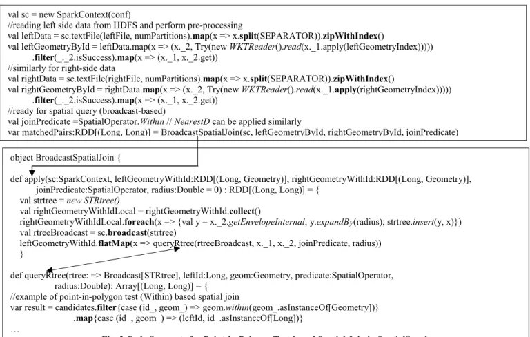
Our experiences on data parallel designs for spatial data processing have greatly sped up the development of Spark-based spatial join query processing, which we call SpatialSpark in this study. Our development of SpatialSpark is motivated by the close correspondences between parallel primitives supported by Thrust library17 (comes with CUDA toolkit18) and Scala vector/collection functions. We refer to our previous works on data parallel designs and their CUDA/Thrust implementations for spatial indexing and spatial joins on GPUs [2, 3]. The Spark platform is able to automatically parallelize and distribute collection methods to multiple computing nodes. This makes parallelization and distributed computing effortless to a certain extent from a developer’s perspective. As an example, Fig. 2 lists the skeleton code for an R-Tree indexed, point-in-polygon test (Within) based spatial join. For readability purpose, Scala collection methods are bolded and external functions implemented in the Java Topology Suit (JTS19) package (more explanation next) are italicized. Clearly, the implementation is much more concise than the equivalent implementations in both SpatialHadoop and HadoopGIS.
Since SpatialSpark is written in Scala, most of Java libraries can be used without any changes. While SpatialSpark has implemented several spatial indexing and spatial filtering techniques, it reuses the popular JTS for spatial refinement, i.e., testing whether two geometric objects satisfy a certain spatial relationship (e.g., point-in-polygon) or calculating a certain
16 https://databricks.com/blog/2014/10/10/spark-petabyte-sort.html 17 https://thrust.github.io/
18 https://developer.nvidia.com/cuda-toolkit 19 http://www.vividsolutions.com/jts/
metric between two geometric objects (e.g., Euclidian distance). In addition to utilizing finer grained data parallelism to achieve higher performance, as all the intermediate data are memory-resident in Spark and SpatialSpark, expensive disk I/Os can be minimized which is a key to achieve the desired high-performance. While we still use strings to represent geometry in SpatialSpark to provide a fair comparison with ISP-MC (See Section 5 for details) as well as make it compatible with existing Hadoop-based systems (e.g. HadoopGIS), it is technically possible to represent geometry in SpatialSpark as binary both in-memory and on HDFS to avoid string paring overheads and allow flexible disk accesses for higher efficiency. This is left for our future work.
Despite the overall high efficiency of Spark at the system level as a development platform (and hence applications based on Spark such as SpatialSpark), we have found that in certain
cases, SpatialSpark can perform worse on multiple computing nodes than on a single node, especially for experiments that are more data intensive. The low scalability may indicate that data communication overheads among distributed computing nodes might be a potential bottleneck. A preliminary investigation reveals that Spark selects a new leader and reconstructs an actor system to exchange the metadata of partitions for every job stage that involves shuffling among distributed computing nodes. The overheads can be significant for relatively small jobs which has also been observed in [14] for experiments on relational queries on key-value stores. As the overheads of metadata communications among distributed nodes are strongly related to the number of partitions in each job stage, this brings an interesting research question on optimizing the number of partitions which represents the tradeoffs between the degrees of parallelisms (the higher the better) and the communication overheads (the lower the better).
IV. ISP-MC:AMULTI-CORE CPUIMPLEMENTATION OF SPATIAL JOIN ON IMPALA
Different from Spark, Impala is designed as an end-to-end system for efficiently processing SQL queries on relational data. A SQL statement is first parsed by Impala frontend to generate a logical query plan. The logical query plan is then transformed into a physical execution plan after consulting HDFS and the Hive metastore to retrieve metadata, such as the mapping between HDFS files and local files and table schemas. The physical execution plan is represented as an
Abstract Syntax Tree (AST) where each node corresponds to an action, e.g., reading data from HDFS, evaluating a selection/projection/where clause or exchanging data among multiple distributed Impala instances. Multiple AST nodes can be grouped as a plan fragment with or without precedence constraints. Impala backend consists of a coordinator instance and multiple worker instances. One or multiple plan fragments in an execution plan can be executed in parallel in multiple worker instances within an execution stage. Raw or intermediate data are exchanged between stages among multiple instances based on the predefined val sc = new SparkContext(conf)
//reading left side data from HDFS and perform pre-processing
val leftData = sc.textFile(leftFile, numPartitions).map(x => x.split(SEPARATOR)).zipWithIndex()
val leftGeometryById = leftData.map(x => (x._2, Try(new WKTReader().read(x._1.apply(leftGeometryIndex))))) .filter(_._2.isSuccess).map(x => (x._1, x._2.get))
//similarly for right-side data
val rightData = sc.textFile(rightFile, numPartitions).map(x => x.split(SEPARATOR)).zipWithIndex()
val rightGeometryById = rightData.map(x => (x._2, Try(new WKTReader().read(x._1.apply(rightGeometryIndex))))) .filter(_._2.isSuccess).map(x => (x._1, x._2.get))
//ready for spatial query (broadcast-based)
val joinPredicate =SpatialOperator.Within // NearestD can be applied similarly
var matchedPairs:RDD[(Long, Long)] =BroadcastSpatialJoin(sc, leftGeometryById, rightGeometryById, joinPredicate) object BroadcastSpatialJoin {
def apply(sc:SparkContext, leftGeometryWithId:RDD[(Long, Geometry)], rightGeometryWithId:RDD[(Long, Geometry)], joinPredicate:SpatialOperator, radius:Double = 0) : RDD[(Long, Long)] = {
val strtree = new STRtree()
val rightGeometryWithIdLocal = rightGeometryWithId.collect()
rightGeometryWithIdLocal.foreach(x => {val y = x._2.getEnvelopeInternal; y.expandBy(radius); strtree.insert(y, x)}) val rtreeBroadcast = sc.broadcast(strtree)
leftGeometryWithId.flatMap(x => queryRtree(rtreeBroadcast, x._1, x._2, joinPredicate, radius)) }
def queryRtree(rtree: => Broadcast[STRtree], leftId:Long, geom:Geometry, predicate:SpatialOperator, radius:Double): Array[(Long, Long)] = {
//example of point-in-polygon test (Within) based spatial join
var result = candidates.filter{case (id_, geom_) => geom.within(geom_.asInstanceOf[Geometry])} .map{case (id_, geom_) => (leftId, id_.asInstanceOf[Long])}
…
execution plan. When a set of tuples (i.e., a row batch) is processed on a data exchange AST node, the tuples are either broadcast to all Impala worker instances or sent to a specific worker instance using a predefined hash function to map between the keys of the tuples and their destination Impala instances. Tuples are sent, received and processed in row batches and thus they are buffered at either the sender side, receiver side or both. While adopting a dynamic scheduling algorithm might provide better efficiency, currently Impala makes the execution plan at the frontend and executes the plan at the backend. No changes on the plan are made after the plan starts to execute at the backend. This significantly reduces communication complexities and overheads between the frontend and the backend which could make Impala more scalable at the cost of possible performance loss. As an in-memory system that is designed for high performance, the raw data and the intermediate data that are necessary for query processing are stored in memory in Impala, although it is technically possible to offload the data to disks to lower memory pressure and to support fault tolerance. An advantage of in-memory data storage in Impala is that, instead of using multiple copies of data in the map, shuffle
and reduce phases in Hadoop, it is sufficient to store pointers to the raw data in intermediate results, which can be advantageous than Hadoop/MapReduce, especially when values in (key,val) pairs have a large memory footprint.
Impala has efficient system infrastructure supports for full table scans and aggregation operations by exploiting several advanced techniques, such as Just-In-Time (JIT) compilation [12] based on the leading open source package LLVM (Low Level Virtual Machines20) and Streaming SIMD Extensions (SSE) that are supported by the Vector Processing Units (VPUs) available on modern CPU hardware [8]. Impala also has an optimized implementation for both broadcast-based and partition-based hash joins which make equi-joins on relational data based on hashing highly efficient. However, extending Impala to support spatial data types and their operations is challenging for several reasons. First, Impala is designed to be an end-to-end system that is ready to use out of the box. As such, functional modules in Impala are tightly coupled. This makes it difficult to integrate additional processing logic that are necessary for supporting new data types and operations. For example, while it is straightforward to load spatial indices from a distributed file system and apply them to filter out spatially non-intersecting data items in Spark, it would require changing both the frontend (to insert AST nodes for loading indices) and the backend (to implement the spatial filtering logic) in Impala, which is non-trivial even for experienced developers. Second, currently Impala has little support for non-equi joins. For example, the current implementation of cross joins can only use a single CPU core per Impala instance, although the computing node executing the instance is likely to be a multi-core machine. Lacking support for multi-core parallel relational joins in Impala has significantly lowered its performance when compared to similar systems (e.g. [13]). In contrast to Hadoop and Spark which essentially treat multiple CPU cores as multiple processors
20 http://llvm.org/
for shared-nothing parallel executions, multi-core CPUs are visible to the Impala backend which makes it attractive to improve system performance by utilizing multiple CPU cores explicitly. However, the technical bar seems to be high to seamlessly integrate native parallelization techniques on multi-core CPUs (e.g., OpenMP and Intel TBB), LLVM JIT techniques employed by Impala and the pull-based asynchronous executions on row batches.
Impala is designed for relational data and does not support user defined data types natively. While we represent geometry as strings to bypass this problem, the solution is inefficient in nature and native support is much more desirable. Since our goal is to evaluate the performance of Impala for large-scale spatial joins rather than significantly extending Impala to natively support new data types and operations (which may require more effort and is left for our future work), we have adopted a non-invasive strategy for the integration. Nevertheless we are aware of the possible inefficiencies and will provide more discussions in Section 6.
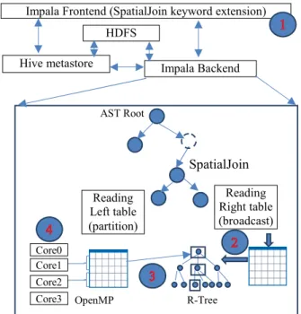
Fig. 3 ISP-MC System Architecture and Components To implement ISP-MC, we first add “SpatialJoin” key word to the Impala frontend to create an AST node after SQL parsing. Correspondingly a subclass of BlockJoin, which we call SpatialJoin, is developed to handle the spatial join logic when the AST node is trigged, in a way similar to
CrossJoin implemented in Impala. Second, since the right
side of a spatial join is broadcast to all Impala instances, we iteratively retrieve all the row batches of the right side table and build an in-memory R-Tree for it, in a way similar to the broadcast hashing-based equi-join for relational data in Impala. Third, we loop through all the tuples in all row batches of the table on the left side of the spatial join and query against the in-memory R-Tree to pair tuples in both left side and right side tables. The paired tuples are written to the in-memory buffer corresponding to the SpatialJoin AST node for outputting. This step is similar to the indexed nested-loop spatial join procedure in spatial database
Impala Frontend (SpatialJoin keyword extension)
Hive metastore Impala Backend
SpatialJoin Reading Left table (partition) Reading Right table (broadcast) HDFS Core0 Core1 Core2
Core3 OpenMP R-Tree
literature [1]. Fourth, to speed up the spatial join query processing, we use OpenMP to parallelize the R-Tree traversals of tuples for row batches. The four components of ISP-MC are illustrated in Fig 3.
Since we represent geometry as strings in the Well-Known-Text (WKT21) format, the strings need to be parsed in three cases: building an R-Tree for all tuples of the table on the right side, probing the R-Tree for all tuples of the table on the left side, and applying user-defined functions (UDFs) for evaluating spatial relationships of paired tuples (spatial refinement) after R-Tree probing (spatial filtering). Currently the UDFs for evaluating spatial relationships (e.g., intersect and contains) are simple wrappers of the corresponding GEOS functions which can be accessed as a shared library. We plan to implement these functions as LLVM Intermediate Representation (IR) code either manually or programmatically in the future for better JIT optimization that is supported by Impala.
V. EXPERIMENTS AND PERFORMANCE EVALUATION In this section, we perform extensive experiments to evaluate the performance of SpatialSpark and ISP-MC. Two commonly used spatial join queries are considered, one is point-in-polygon test based spatial join (Within) and the other is to find nearest polyline within a predefined distance (NearestD) for each point.
A. Setup
We allocate a cluster consisting of 10 g2.2xlarge EC2 instances from Amazon for our experiments. Although technically multiple EC2 instances can be virtualized on the same physical computing node, we use instances and computing nodes (or simply nodes) interchangeably for notation convenience. Each EC2 node has 8 vCPUs, 15 GB memory and 60 GB SSD. We install Hadoop 2.5.0 from Cloudera CDH 5.2.0 with default settings on the cluster. We use Spark 1.1.0 which is the latest version at the time of writing. We also configure an in-house high-end machine as a single node cluster to test the infrastructure overheads in both SpatialSpark and ISP-MC. The machine has 16 CPU cores and 128GB memory and uses the same software stack as in the EC2 nodes.
The first point dataset is derived from pickup locations of NYC taxi trip data [2] and has ~170 million points (termed as taxi dataset). To experiment the Within spatial join, we use a polygon dataset from New York City census block data22 with about 40 thousand polygons (termed as nycb dataset). For the nearest neighbor search (NearestD), we use NYC street network (LION23) dataset that has about 200K polylines (termed as lion dataset). All datasets are formatted and stored in text files in HDFS with geometries (points, polylines and polygons) in WKT format. The data volumes of the taxi, nycb and lion datasets in HDFS are 6.9GB, 18.7 MB and 29.0 MB, respectively. The average number of polygon vertices of nycb is about 9. We use taxi-nycb and
taxi-lion pairs to label the two experiments, respectively.
21 http://en.wikipedia.org/wiki/Well-known_text
22 http://www.nyc.gov/html/dcp/html/census/census_2010.shtml 23 http://www.nyc.gov/html/dcp/html/bytes/dwnlion.shtml
In addition to the taxi point dataset, we also prepare a subset of the GBIF species occurrence data. We extract about 10 million occurrences and formatted their geometry as WKT strings (termed as G10M dataset). The World Wide Fund global ecoregions24, which have 14,458 polygons and 4,028,622 vertices (279 vertices per polygon on average), is used as the right side dataset (termed as wwf dataset) for point-in-polygon test (Within) based spatial joins and the experiment is labeled as G10M-wwf. The data volumes of the
G10M and wwf datasets in HDFS are 290.5MB GB and 149.8 MB, respectively.
B. Results of single-node Performance
We first experiment the three spatial joins, i.e., taxi-nycb
(Within), taxi-lion (NearestD) and G10M-wwf (Within), on a single computing node using both SpatialSpark and ISP-MC. For the taxi-lion experiment, we use two distance values (D) (100 feet and 500 feet) and label them as taxi-lion-100 and
taxi-lion-500, respectively. Conceptually, the larger the
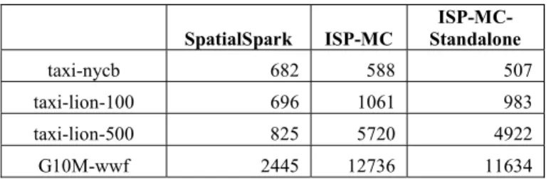
distance value, the more computation workload. The results are listed in the first two columns of Table 1.
Table 1 Runtimes (IN SECONDS) on a Single Node SpatialSpark ISP-MC Standalone
ISP-MC-taxi-nycb 682 588 507
taxi-lion-100 696 1061 983
taxi-lion-500 825 5720 4922
G10M-wwf 2445 12736 11634
From the results, we can observer that SpatialSpark is generally faster than ISP-MC, especially in the taxi-lion-500
experiment where SpatialSpark is almost 7X faster than ISP-MC. This is somewhat unexpected as we expected a native C++ implementation is typically faster than a Java implementation. Further investigations suggest that the performance difference is largely due to two factors. First, for geometric operations in the spatial refinement phase of the spatial joins, which dominate the overall overheads in the experiments, SpatialSpark uses the JTS library while ISP-MC uses GEOS. Although GEOS is a language port of JTS, our experiments using 10 thousand samples from the taxi and
gbif datasets (termed as taxi10k and gbif10k, respectively) in a standalone mode (without using Spark or Impala) show that JTS is much faster than GEOS for the “Within” operation: 3.3X for taxi10k-nycb and 3.9X for gbif10k-wwf. While it is beyond our scope to provide a comprehensive analysis of the performance difference between JTS and GEOS, we found that GEOS frequently creates and destroys small objects to minimize memory footprint (which is actually unnecessary for modern computers with GBs memory). The operations are cache unfriendly and are very expensive on modern CPUs. Second, the four spatial join experiments also suggest that the static scheduling used by Impala might be a bottleneck for unbalanced spatial joins. As the numbers of polyline/polygon vertices can vary
24http://www.worldwildlife.org/biomes
significantly, the workloads assigned to OpenMP threads (within a row batch) can be unbalanced which hurts ISP-MC performance quite a lot. Note that we were forced to use static OpenMP scheduling due to thread safety issues in the GEOS library and the way Impala uses LLVM JIT, although we are aware that using dynamic scheduling (or TBB multi-threading which uses work-stealing) might achieve better load balancing and better performance.
To further understand the system infrastructure overhead of Impala, we implement a standalone version of ISP-MC. The results are listed in the last column of Table 1. When comparing ISP-MC with its standalone version, the system infrastructure overheads, which are 13.7%, 7.3%, 13.9% and 8.7% in the four experiments, are reasonable. Although Spark has a “local” mode which is conceptually similar to the standalone implementation for ISP-MC, we found that the performance difference between the single-node configuration and the “local” mode configuration for SpatialSpark is insignificant which makes the comparison uninteresting. We have also tested a native Scala parallel implementation for point-in-polygon test (Within) based joins on a single node (without using Spark), which might be more comparable to the standalone implementation of ISP-MC. However, the native Scala parallel implementation uses excessive memory and performs rather poor which makes the comparison uninteresting as well. While more investigations are needed, it seems that both Impala and Spark provide good infrastructure supports for our spatial extensions. However, the low performance of GEOS for geometric operations in spatial refinements, whose computations typically dominate spatial join query processing, makes SpatialSpark perform significantly better than ISP-MC.
C. Results of Cloud Performance
We evaluate the performance of the four experiments on a 10-node Amazon EC2 cluster. The results are listed in Table 2. Similar to the single node performance, SpatialSpark is about 4.7X-10.5X faster than ISP-MC on the 10-node cluster. In addition to the different performance of the underlying geometry operation libraries (JTS for SpatialSpark and GEOS for ISP-MC) and the intra-node load unbalancing due to OpenMP static scheduling, the static inter-node scheduling adopted in Impala might be an important factor in the increasing performance difference between SpatialSpark and ISP-MC on the 10-node cluster. We observe that some Impala instances take much longer to complete the spatial joins than others. In contrast, Spark is able to distribute the workload dynamically to computing nodes which results in better load balancing in distributed computing environments.
TABLE 2RUNTIMES (INSECONDS) USING 10EC2NODES SpatialSpark ISP-MC
taxi-nycb 110 758
taxi-lion-100 65 307
taxi-lion-500 249 1785
G10M-wwf 735 7728
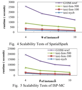
We also perform scalability tests for the four experiments by varying the numbers of computing nodes from 4 to 10. We are not able to use fewer than 4 nodes for the experiments due to the memory limitation of the EC2 instances (15 GB per node). The scalability results for SpatialSpark and ISP-MC are plotted in Fig. 4 and Fig. 5, respectively. As the number of computing nodes increases from 4 to 10 (2.5X), SpatialSpark speedups vary from 1.97X to 2.06X. The parallel efficiency, which is calculated as the ratio of performance speedup over increase of parallel processing units, is about 80%. ISP-MC shows almost linear scalabilities for all the four experiments (parallel efficiency close to 100%) except in the case when the number of computing nodes is increased from 8 to 10 in the G10M-wwf
experiment where the runtime is reduced from 6357s to 6257s only. This is likely due to the increasing inter-node load unbalancing in ISP-MC as discussed previously.
Fig. 4 Scalability Tests of SpatialSpark
Fig. 5 Scalability Tests of ISP-MC VI. DISCUSSIONS
SpatialSpark and ISP-MC represent two very different realizations on processing spatial join queries on top of existing Big Data system infrastructures. On one side, SpatialSpark is API-driven, relies on programming language (Scala) and platform (Spark) for (semi-) transparent parallelization and distribution, and uses virtual machines (JVM) for portability at the expense of efficiency. On the other side, ISP-MC is more like a plug-in to Impala, which both enjoys the efficiency provided by the underlying platform and suffers from significant limitations imposed by the platform.
From a developer perspective, it takes a lot more efforts to understand the overall structure of the Impala system as well as several underlying advanced techniques, e.g., data communication between the frontend and backend, the correspondence between AST nodes and their related C++ classes, the fundamental role of the row batch structure in determining data flows between parent and child AST nodes,
0 500 1000 1500 2000 2500 3000 4 6 8 10 ru nt im e ( secon ds ) # of instances G10M-wwf taxi-lion-500 taxi-lion-100 taxi-nycb 0 5000 10000 15000 20000 25000 4 6 8 10 ru nt im e ( secon ds ) # of instances G10M-wwf taxi-lion-500 taxi-lion-100 taxi-nycb
multi-threaded disk I/Os, and the way the JIT compilation technique is integrated. In contrast, the majority of the techniques that are related to parallelization/distribution and data communication are nicely abstracted away either by Spark or by the modules that it depends on (e.g., Akka and Netty). As a result, developers can focus on domain specific logic (spatial indexing and filtering in particular in this study). Despite that the experiments in Section 5 have shown SpatialSpark to perform better than ISP-MC, which can be attributed mostly to better performance of geometry library (JTS vs. GEOS) and dynamic scheduling, a native implementation of spatial joins on top of the Impala infrastructure has several unique advantages in better exploiting hardware capabilities. These advantages, including high-performance disk I/O, JIT-based machine code optimization, native multi-threading on multi-cores, Single Instruction Multiple Data (SIMD, [8]) hardware accelerations, in addition to native machine code execution, are important for our future extensions.
As for Cloud deployment, software tools are available to automatically deploy compiled packages to Cloud computing resources in both Spark and Impala. While it may take more efforts to compile C++ source code to shared libraries (for spatial indexing/join logic) or IR code (for UDFs) and install them properly in all Impala instances, which are one-time costs, we observe that there is a per-run overhead to pack Jar files and send them to work instances in Spark. The overhead can be significant when multiple large Jar files are required. Refactoring the Jar files to include only Java classes that are being used will likely reduce the overhead. From a user perspective, while SpatialSpark takes command line arguments and requires HDFSs files paths as inputs for spatially joining two datasets, ISP-MC takes spatially extended SQL statements, which could be preferable for users who are more familiar with SQL.
We believe that it is technically possible to factorize Impala into several loosely coupled modules, such as SQL parsing, scheduling, distributed data communication and asynchronous multi-threaded disk I/Os. These modules can expose necessary APIs to developers after proper abstractions. The factorization will allow developers to relatively easily integrate indexing and operations for new data types while reusing existing infrastructure modules for distributed data management. We are in the process of exploring the possibility of developing a Big Data system that natively supports semi-structure data models. We plan to begin with spatial data and focus on spatial joins. Understanding the advantages and limitations of existing Big Data systems is the first step towards the goal, which largely motivates the work reported in this paper.
While it is beyond the scope of this paper to provide a detailed report on the individual factors that affect the performance of Impala and Spark on modern commodity parallel hardware with respect to programming languages (C++ vs. Scala), thread coordination (sharing memory variables across threads vs. completely independent), runtime systems (native execution vs. virtual machines), disk I/Os (shared buffer pool among multiple threads vs.
independent), network communications (interface definition based vs. actor/message based and synchronous vs. asynchronous) and scheduling strategies (static vs. dynamic), we believe our reference implementations of SpatialSpark and ISP-MC and their performance evaluations can provide valuable guidance for our future Big Data system design and development as well as for similar research and development efforts.
VII.CONCLUSION AND FUTURE WORK
In this study, we have reported our designs and implementations of two prototype systems, namely SpatialSpark and ISP-MC, for large-scale spatial join query processing in Cloud. Experiments using multiple real datasets on a 10-node Amazon EC2 cluster have demonstrated good scalability. For future work, in addition to those have been discussed in the previous sections, first, we would like to boost the performance of geometry operations by integrating the data parallel designs, which are also efficient on multi-core CPUs [2], into ISP-MC. Second, we would like to reduce memory footprints for spatial join query processing in both SpatialSpark and ISP-MC, which are largely inherited from Spark and Impala and are increasingly becoming a bottleneck. Finally, we would like to apply similar designs to other non-relational data types, such as trajectory data.
ACKNOWLEDGEMENT
This work is supported through NSF Grants IIS-1302423 and IIS-1302439. REFERENCES
1. E. H. Jacox, and H. Samet (2007). Spatial join techniques. ACM Transaction on Database System 32(1), Article #7.
2. J. Zhang, S. You and L. Gruenwald (2014). Parallel Online Spatial and Temporal Aggregations on Multi-core CPUs and Many-Core GPUs," Information Systems, vol. 4, 134–154.
3. Zhang, J. and You, S. (2012). Speeding up large-scale point-in-polygon test based spatial join on GPUs. In Proc. ACM BigSpatial, 23-32. 4. A. Eldawy and M. Mokbel (2013). A demonstration of Spatialhadoop: an
efficient mapreduce framework for spatial data. in Proc. VLDB, 6(2), 1230-1233
5. A.Aji et al (2013) Hadoop-GIS: A High Performance Spatial Data Warehousing System over MapReduce. In Proc. VLDB, 6(11), 1009-1020, 2013.
6. J. Dean and S. Ghemawat (2010). MapReduce: a flexible data processing tool. Communications of the ACM 53(1):72-77
7. R.Appuswamy, C. Gkantsidis et al. (2013). Scale-up vs Scale-out for Hadoop: Time to rethink?. In Proc. SOCC, Article #20.
8. J. L. Hennessy and D. A. Patterson (2011). Computer Architecture: A Quantitative Approach, 5th edition. Morgan Kaufmann.
9. X. Xie, Z. Xiong et al (2014). On Massive Spatial Data Retrieval Based on Spark. Proc. WAIM, 200-208.
10. M. Zaharia, M. Chowdhury et al (2010). Spark: Cluster Computing with Working Sets. In Proc. HotCloud.
11. K. A. Kumar et al (2014). Optimization Techniques for "Scaling Down" Hadoop on Multi-Core, Shared-Memory Systems," in Proc. EDBT. 12. S. Wanderman-Milne and N. Li (2014). Runtime Code Generation in
Cloudera Impala. IEEE Data Engineering Bulletin,37(1), 31-37.
13. S. Zhang, Y. Yang et al (2014). OceanRT: Real-Time Analytics over Large Temporal Data. in Proc. SIGMOD, 1099-1102.
14. H.Zhang, B. M. et al (2014). Efficient In-memory Data Management: An Analysis. in Proc. VLDB, 833-836.