Farm size and cost relationships in relation to recent machine technology: An analysis of potential farm change by static and game theoretic methods

Volume 34

Number 504

Farm size and cost relationships in

relation to recent machine technology

Article 1

May 1962

Farm size and cost relationships in relation to recent

machine technology: An analysis of potential farm

change by static and game theoretic methods

Earl O. Heady

Iowa State University of Science & Technology

Ronald D. Krenz

Iowa State University of Science & Technology

Follow this and additional works at:

http://lib.dr.iastate.edu/researchbulletin

Part of the

Agriculture Commons

,

Economics Commons

, and the

Sociology Commons

This Article is brought to you for free and open access by the Iowa Agricultural and Home Economics Experiment Station Publications at Iowa State University Digital Repository. It has been accepted for inclusion in Research Bulletin (Iowa Agriculture and Home Economics Experiment Station) by an authorized editor of Iowa State University Digital Repository. For more information, please [email protected].

Recommended Citation

Heady, Earl O. and Krenz, Ronald D. (1962) "Farm size and cost relationships in relation to recent machine technology: An analysis of

potential farm change by static and game theoretic methods,"Research Bulletin (Iowa Agriculture and Home Economics Experiment

Station): Vol. 34 : No. 504 , Article 1.

Farm Size and Cost Relationships

in Relation to Recent Machine , echnology

An Analysis of Potential Farm Change

By Static and Game Theoretic Methods

by Earl O. Heady and Ronald D. Krenz Department of Economics and Sociology

Center for Agricultural and Economic Adjustment cooperating

AGRICULTURAL AND HOME ECONOMICS EXPERIMENT STATION

IOWA STATE UNIVERSITY of Science and Technology

CONTENTS

Summary ... 444

Introduction ... 445

Objectives ... ~ ... 445

Budget technique ... 446

Per-unit cost cuzves ... _ 446 Costs of inputs ... _ ... _ ... _ ... 447

Prices and yields ... 447

Timeliness of operations ... 447

Cost functions for various machinery combinations and current cropping systems ... 448

Costs per unit of product ... 449

Relationship of cost functions to cropping system ... 452

Costs under a 5-year rotation program ... 452

Effect of fertilizer application level on per-unit costs for Carrington-Clyde soils ... 453

Per-unit costs under a continuous-corn program on Carrington-Clyde soils ... 455

Comparison of cost functions for two soil types ... 455

Effects of price changes on cost schedules ... _ ... 457

Cost functions at different price levels on Carrington-Clyde soils ... 457

Size in acreage with product price changes ... 457

Break-even prices on Carrington-Clyde soils ... 458

Residual returns to labor and land ... _... 458

Comparison with nonfarm labor incomes for Carrington-Clyde soils ... 458

Land returns ... 459

Optimum acreage under weather variations, Carrington-Clyde soils ... 460

Game theoretic criteria applied to Carrington-Clyde soils ... 462

Decision criteria ... 462

Determination of optimum machinery investment for a given acreage ... 463

SUMMARY

This study includes estimates of the relation of more recent machine technology to per-unit costs of crop production for farms of different sizes. The types of new machine technology of particular interest in-clude large-capacity equipment such as 4- and 6-row corn planting and cultivating equipment and picker-sheller harvesting machines. A hypothesis generally held by persons concerned with agriculture is that these large-capacity machines, with high fixed costs which must be spread over more acres, stand to cause an important increase in farm size.

This study is based on data for the Carrington-Clyde soils in northeast Iowa and the Ida-Monona soils in western Iowa. Cost functions are estimated for farms of different sizes or acreages by budgeting procedures. More specifically, cost curves are derived as a function of acreage per farm. Losses in crop production result-ing from untimely field operations are considered as costs for different acreages and are related to particular machine combinations. Parametric linear programming is used to permit analyses of livestock optimum enter-prises and to consider the effect of subjective discount-ing of returns on size considerations. For decision making under risk and uncertainty, game theory models were employed to incorporate consideration of weather variations on optimal machinery-land or farm-size relationships.

The results, assuming average weather and current cropping methods, indicate that cost advantages associ-ated with 6-row cropping equipment and field corn shellers are small relative to more standard sizes and types of machines. An expansion of farm size from 200 acres operated with 2-row equipment to 400 crop-acres operated with 4-row equipment is estimated to reduce costs by 6 cents per $1 of crop product pro-duced. Expansion to 600 crop-acres operated by 6-row equipment would further reduce costs by only 1.5 cents per dollar of crop product.

Under a farm organization including cash cropping and current rotations, minimum per-unit production costs (per dollar of product) are attained in the range of 600 to 680 crop-acres. However, the reduction in per-unit costs is small as acreage is extended from 400 to 800 crop-acres. With a continuous-corn rotation, minimum per-unit costs are attained at a size of 320 crop-acres.

The static budgeting analysis indicates that, while small cost reductions are possible as machinery invest-ment is increased and as crop acreage is expanded beyond 320 acres, these savings alone probably are not great enough to "force" much larger farms. The greatest reduction in cost per unit of product is attained at approximately 320 acres. Up to this point, the high fixed costs of modern machinery decline rapidly as acreage and output are extended. For example, with fixed costs of $1,000, an expansion in acreage from 10 to 20 lowers fixed cost per acre from $100 to $50. An expansion from 400 acres to 800 acres, however, with fixed costs remaining at $1,000, lowers per-acre

444

fixed cost from $2.50 to $1.25, a reduction of much less absolute importance, even though of the same relative magnitude. Too, cost functions were calculated on the basis of a charge for all labor. On smaller farms, a greater proportion of the labor would be provided by the family at a lower opportunity cost. This is a general type of finding under the static cost analysis of this study. While slight cost reductions can be attain-ed by larger machine combinations and greater acreages, considerations such as capital availability and ability of farmers to withstand risks will be more important than current cost reduction possibilities in bringing about larger farms. Or, the possibilities might be stated other-wise: Just as a farm with 320 crop-acres has no great cost advantages when compared with a larger acreage, large farms also have no particular cost disadvantages when compared with smaller ones which may rely on more unpaid family labor.

A consideration of the yearly weather variation and days suitable for field operations indicated that an analysis based on average weather causes long-run unit production costs to be underestimated. Low per-unit costs in favorable weather are outweighed by extreme crop losses in years of unfavorable weather if only average weather is assumed. Hence, optimal machinery investment per acre to meet weather varia-tions is higher than would be necessary if weather were static among years. The use of field corn shellers, found not to be profitable with less than 800 crop-acres when average weather is assumed, is estimated to be profitable on 450 acres when variations in weather are considered in cost and return calculations. These machines may prove profitable even on smaller acreages when decision is based on uncertainty criteria.

Several game theoretic criteria were applied in the examination of optimum farm size under uncertainty. The strategy selected by the 'Wald maximin criterion, a conservative model, is that which gives maximum expected profits under supposition of the least favor-able weather. The specified acreage is 520. The Savage minimax-risk criterion, a strategy which minimizes the maximum risk, specifies a falm size of 560 acres. The Hurwicz pessimism-optimism index specifies different acreages, depending on the particular index, oc, chosen. The index, oc, is an indication of the degree of opti-mism (or pessiopti-mism) held by the decision maker. With values of 0.4 to 1.0 assigned to oc, the optimum size is 520 acres. But with minimum pessimism and a value of zero assigned to oc, the optimum acreage is 720 with investment in machinery accordingly.

When these same game theoretic techniques were applied to decision making under uncertainty, it was found that a larger machine investment proved optimal than was true when analysis was based on static budget-ing approaches. For example, the static budget ap-proach specified only 2-row machinery for a 200-acre farm. When game models were applied under assump-tions of weather variation and uncertainty, however, 4-row machinery proved to be optimal.

Farm Size and Cost Relationships

In Relation to Recent Machine T echnologYl

An Analysis of Potential Farm Change

by Static and Game Theoretic Methods

by Earl O. Heady and Ronald D. Krenz

Farmers operate in a dynamic environment which is characterized by continual change and adjustment. One of the problems of change which confronts farmers is that of determining the proper combination of re-sources to use in production. Machines of large capacity, such as 6-row field equipment and picker-shellers for corn, are now on the market and are in use on numer-ous Com Belt farms. Hence, farmers are faced with the question: "What combination of land, labor and machinery (i.e., what size of farm) is optimum or desirable in this situation?" This study includes analy-ses to provide quantitative information on the relation-ship of unit costs of production for farms of different sizes when operated with farm machinery of varying capacities. This information should be useful to farmers making decisions on whether to adopt machine tech-nology such as that represented by 4-row and 6-row com equipment and field com shellers. It should pro-vide data indicating sizes of farms which are optimum for machine combinations with varying field capacities, investment costs and possibilities in labor substitution. In addition, to aid in individual farmer decisions, empirical analyses of the type explained in this study provide information suggestive of the upcoming struc-ture of farming. While the process is slow and gradual, farm size has continuously adjusted to new cost struc-tures and the substitutability of machine capital for labor. This study, designed to indicate acreage ranges over which new machine technology gives lowest unit costs of production, should suggest the minima toward which farm size may trend. There are, of course, other variables which affect both machine and farm sizes. For example, revolutionary changes in farm size did not occur in the shift from horse power to tractors because not all farmers were inclined, or forced, to change their scale of operations. Farmer age, lack of capital and other variables restrained the rate at which these techniques were adopted. The same is likely for other machine techniques now appearing.

OBJECTIVES

The major purpose of this study is to determine per-unit cost relationships associated with various machinery techniques. Unit costs of production are 1 Project 1328, Iowa ~ricultural and Ho~e E~nomics Experi,,!ent . Station, Center for AgrIcultural and EconomiC Adjustment cooperatmg.

determined for farms of different acreages under more recent machine technology as well as under the types and sizes of crop equipment and power units now in use on the majority of Iowa farms. Comparison is made of cost functions under upcoming and existing machine technology to suggest the cost advantages which mayor may not exist between them. The data generated are used to analyze both the acreage which results in lowest per-unit costs of production and the optimum farm size in terms of profit maximization.2 Use of recent machinery techniques, such as 6-row corn equipment and picker-shellers, requires relatively large farms for profitable crop production. Hence, it is pos-sible that minimum per-unit costs for these newer machines mayor may not differ greatly from the minimum per-unit costs possible with more conventional machinery on farms of typical sizes in Iowa, depending on the size of farm on which the machines are employed. As part of the more general objective of this study, the following are specific objectives in relating machine techniques to cost relationships and farm size:

1. To determine the magnitude of cost economies associated with various machinery techniques.

2. To determine the sizes of farms which allow at-tainment of minimum per-unit production costs for each of the several sizes of machinery analyzed. (The study also includes determination of farm size necessary to allow attainment of the majority of the cost econ-omies associated with various types of machines.)

3. To compare information on costs and farm size for various soil, rotation and fertilizer situations.

4. To compare residual returns to labor and land for farms operated with' various sets of machinery, under various price conditions and for various cropping techniques. (This information is provided to suggest the size of operations necessary to give returns on farm resources comparable with rates of returns for resources employed in nonfarm industries.)

5. To examine the effects of weather variations upon the optimal level of machinery investments and optimal farm size.

The purpose of this study is not that of specifying the size of farm which "ought to exist" in Iowa 'or the Corn Belt. Neither is it to predict the average size or 2 The criterion of optimum farm size used is defined as the size at which the marginal costs incurred with the last acre added are equal to the marginal returns from this last acre. At this acreage, profits are maximized. In the long run, under pure competition and adequate knowledge, this also would be the size of farm with minimum average total costs.

the distribution of sizes which might exist at some future time. Rather, it is to provide general informa-tion relating' to per-unit producinforma-tion costs when farms of different sizes are operated with different combina-tions of machines and power units. Cost and related estimates are not made for farms of discrete sizes. In-stead, costs are estimated in the manner of cost curves or functions as acreage is increased against given com-binations of machinery.

BUO'GET TECHNIQUE

This section describes the budget method used in estimating cost relationships for farms organized to produce only cash crops. Cost curves are developed for eight complete sets of farm machinery. Each set includes a slightly different combination of equipment. Together, the various machine combinations cover a wide range of field capacities and investment costs.

The cost curves apply to the soil areas shown in fig. 1. Emphasis in this study is on Carrington-Clyde soils in northeast Iowa. Land in this soil association has a relatively high agronomic rating for corn produc-tion. Intensive cropping is possible since the soil is not greatly subject to erosion.

The Ida-Monona area included in the study repre-sents somewhat the opposite extreme. It borders the Missouri River bottoms and includes a belt of hilly land with steep slopes. The erosion hazard is severe on these soils, and the agronomic rating for corn production is considerably below that of the Carrington-Clyde soils. Hence, a greater proportion of the cropland must be kept in meadow, and cash-grain farming is not as suitable as in the Carrington-Clyde area. Cost curves developed for Ida-Monona soils are based on the use of conservation practices necessary to control erosion and to maintain crop yields over the long run. Cost curves for the various sets of machinery on Carrington-Clyde soils are developed under three crop-ping systems. These cropcrop-ping systems include the cur-rent cropping system as indicated from the 1954 census, a 5-year rotation and a continuous-corn system. A combination of two rotations is used in budgeting cost curves for Ida-Monona soils. The current cropping

sys-Fig. I. Soil assoo::iation areas of Iowa o::onsidered in this study.

446

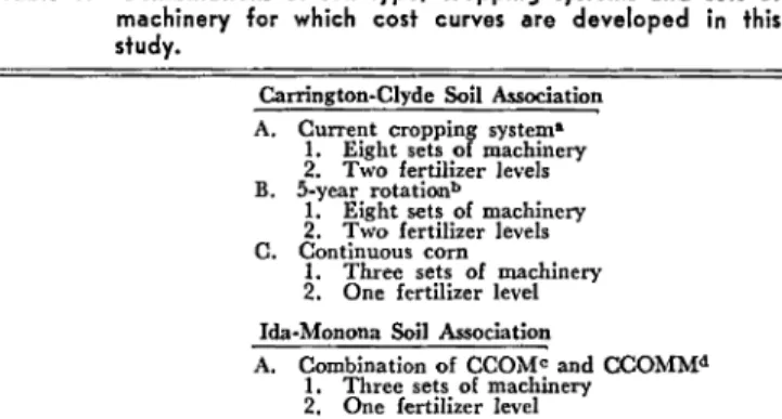
Table I. Combinations of soil type, o::ropping systems and 'sets of mao::hinery for whio::h o::ost o::urves are developed in this study.

Carrington-Clyde Soil Association A. Current cropping system"

1. Eight sets of machinery 2. Two fertilizer levels B. 5-year rotationb

1. Eight sets of machinery

2. Two fertilizer I.vels a. Continuous corn

1. Three set. of machinery 2. One fertilizer level Ida-Monona Soil Association

A. Combination of CaOM. and CCOMMd

1. Three sets of machinery

2. One fertilizer level

• Based on U. S. Census of Agriculture: 1954. l,part 9. 1956.

b Includes 2 years of corn, 1 year of com or soybeans, 1 year of oats and I year of meadow.

• Corn-com-oats-meadow rotation assumed for slopes of 0-13 percent.

d Rotation assumed for slopes of 14 percent Or more.

tern places approximately 51 percent of the land in row crops; the 5-year rotation calls for 60 percent in row crops, and the continuous-corn program calls for placing all land in row crops. Table 1 outlines the cropping systems, fertility levels and machinery com-binations for which cost curves are developed.

Total cost curves are developed for each set of machinery under the various cropping systems. Expan-sion of acreage for a given set of machinery requires that some field operations be performed at unfavorable times. If acreage is increased sufficiently, crops must be planted, tended and harvested so late that yields are depressed. Such "untimeliness" losses are included in the calculation of cost per unit of production for the various acreage ranges. Total costs include annual fixed machinery costs, variable machinery inputs and costs of other variable inputs. A description of these costs and a description of the method of estimating untimeliness losses follow.

Per-Unit Cost Curves

Per-unit cost curves are determined for eight sets of machinery with current cropping methods and the 5-year rotation on Carrington-Clyde soils. Each set of machinery has a somewhat different capacity for field crop operations. All machinery combinations assume the same hay harvesting operations, with the exception that baling is custom hired for the smallest set of machinery. Three of the machine combinations have one tractor and are designed for operation by one man. The

re-maining five sets include two tractors. For the two-tractor machinery combinations, hourly labor is hired to operate the second tractor. The key to these machine combinations is given in table 2. The numbers and

Table 2. Legend and machine o::ombinations used.

Key No. of Tractor

tractors capacity

~: ~:~l~~~: t~~:

::::::::::::::::=::::=:J

3. 4-plowA 4-row ... _ .. _ ... _ .. _ .. .1

4. 3- & ;)-plow, 4-row ... .2 5. 3- & 4-plow, 4-row ... _ ... 2

6. 3- & 4-plow, 6·row ... _ ... 2

7. 3- & 4-plow, combine-picker 2

8. 3-& 4-pIow, picker-sheller .... 2

2-plow 3-plow 4-plow 3-plow 4-plow 4-plow 4-plow 4-plow Planting & cultivating equipment Com harvesting equipment 2-row 4-row 4-row 4-row 4-row 6-row 4-row 4-row

I-row pull type 2-row mounted 2-row mounted 2-row mounted 2-row mounted 2-row mounted Combine-picker Picker-sheller

references at the left are those used later to identify the several machine combinations. Information in other columns refers to the number of tractors included in each set, the plow capacity of the tractors, the size of machinery and the harvesting equipment.

Cost curves also are developed with three machinery combinations for a continuous-com cropping program on Carrington-Clyde soils. These three sets of machinery differ from the eight sets previously discussed since machinery is only required for com operations. Three sets of machinery are also designed for use on Ida-Monona soils. These combinations differ from any combinations designed for Carrington-Clyde soils since some special machines "are required for erosion control.

CostS' of Inputs

For the calculations which follow, input costs are divided into annual fixed costs, which vary with the number of crop-acres operated, and variable costs, which vary with the amount of product produced per acre. The curves so developed are short-run cost curves where machinery is the fixed resource or restraint. Fixed costs which do not vary with acreage or output include annual fixed machinery expenses and depreciation, as well as the overhead labor required for machine main-tenance. Variable costs include those for machinery, fuel, land taxes, labor, cropping expenses (such as seed and fertilizer) and others which vary with the numbers of acres operated and the yield levels attained. Variable costs per unit of output, including transportation and corn drying, are not constant per acre since untimeliness of operations causes yields to decrease as acreage is expanded for a given set of machinery.

FIXED COSTS

Fixed machinery costs include interest, taxes, in-surance, housing and depreciation. An interest charge of 7 percent on machine investments is used in this study since it is the typical rate on loans for machinery purchases. The 7-percent charge is assessed against the "average value" of all machinery. The average value is defined as equal to half of the sum of the purchase price, less 10 percent of the purchase price (trade-in value). An annual charge, varying by type of equip-ment but averaging approximately 2 percent of the original purchase price of machinery, is made for housing, taxes and insurance.

" Depreciation charges include fixed and variable components. The fixed component is based on ob-solescence and "normal annual depreciation" and is obtained by dividing 90 percent of the purchase price by the estimated maximum years of service. Dividing 90 percent of the purchase price by maximum units of service gives the depreciation charge per service unit.

VARIABLE COSTS

Variable costs relative to the number of acres oper-ated include property tax on land, variable machinery costs, labor costs and cropping costs. Property taxes are $2.01 per crop-acre in the Carrington-Clyde area and $2.95 per crop-acre in the Ida-Monona area.8

I Iowa State Tax Commission. Annual report, 1956-57.

Variable machinery costs include fuel, repairs and extra depreciation charges for above-normal annual use. Annual charges for repairs and service are deter-mined as percentages of the machine investment. ""

Variable labor costs include labor required for main-tenance and repair in addition to the actual field operations. Variable maintenance requirements are based on estimates prepared by Hinton.4 _{Labor required}

for actual field operations is equal to the number of tractor hours required. All labor, both maintenance and field operations, for operator or hired labor, is charged at the rate of $1 per hour.

Variable cropping costs include seed, fertilizer and any custom charges required. Variable handling costs include costs of transporting products to market and drying or shelling com. The transport cost is estimated at 3" cents per bushel on all grain crops and 3 cents per bale of hay or straw. For machinery combinations which include field shelling of com, the drying cost is 10 cents per bushel. With conventional com picking, drying costs are replaced by shelling costs of 3 cents per bushel. All per-unit costs are assessed to the produc-tion remaining after subtracting losses resulting from untimely field operations.

Prices and Yields

The per-unit cost curves formulated in this study measure costs per dollar value of crop product, instead of costs per physical unit of product since several crops or products are involved. Hence, prices are needed to determine total value of output. Three sets of prices are used in estimating sizes of farms which are optimum in terms of profit maximization. The three price levels, averages of recent periods, are for 1953-57, 1956-58 and for 1958. Prices during the 1953-57 period average the highest of the three levels chosen. In this period, com price averaged $1.30 per bushel. During the 1956-58 period, the com price averaged $1.13 per bushel. The 1958 average prices are lowest of the three levels with com price at 97 cents per bushel. Average prices for other crop products for each period are provided in the appendix.

Yields assumed for the current cropping program on Carrington-Clyde soils are the average of 1953-57 actual yields in the area. Yields and fertilizer require-ments for other rotations on Carrington-Clyde soils were provided by agronomists.5

Timeliness of Operations

The only factor considered in this study which can result in rising per-unit costs and thus limit the expan-sion of farm size is the untimeliness element of field operations. No other factors are included which result in increasing costs per acre with the expansion of farm size. Other factors which, in practice, will limit farm size (such as limitations of management, land supplies or labor supplies), are omitted from this analysis be-cause these items cannot be readily measured.

Estimates of total production include losses in

• R. A. Hinton Farm management manual. D1. Agr. Ext. Servo But. AE-3349. 1959.

yields because of untimely operations which may arise during the following operations: (1) corn planting, cultivating and harvesting, (2) oats planting and har-vesting, (3) soybean planting and (4) hay harvesting. Estimates of the rate of loss occurring when operations are performed during a suboptimal period were obtain-ed from various agronomic and engineering sources. Loss functions were developed to consider both a "no loss" period and the subsequent crop yield losses which occur as operations are extended beyond this "no loss" period (i.e., if operations are extended into a suboptimal period with respect to seasons of the year).

Several items of information are needed to deter-mine the losses resulting from untimely operations: (1) hours of machinery input required per acre for each cropping operation, (2) hours available in each day for field operations, (3) the period over which opera-tions can be performed without losses (the optimal period) and (4) estimates of the losses that occur as an increasing function of time if operations are perform-ed during the suboptimal period.

Average dates for beginning each operation and the time limitations on the optimal period for operations were obtained from a survey among county extension directors in the respective soil areas. Estimates of the number of days available for field operations were ob-tained from .records of the Agronomy Farm at Ames and were adjusted to the conditions of northeastern and western Iowa.

COST FUNCTIONS FOR VARIOUS

MACHINERY COMBINATIONS AND

CURRENT CROPPING SYSTEMS

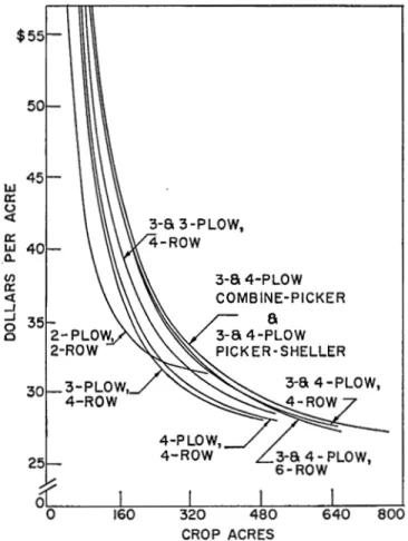
Cost curves for eight sets of machinery, based on current cropping methods in the Carrington-Clyde area and 1953-57 prices, are presented in this section. The first cost curves presented are on a per-acre basis and merely show the costs per acre as the number of acres is increased for a given set of machinery. Account is not taken of loss resulting from untimeliness of opera-tions. Per-acre cost curves fall rapidly over small acre-ages because of the dominance of fixed costs. As acreage is extended, however, per-acre costs are composed of

an inc~eas~ng proportion of variable costs. The slope

or dechne m the cost curves decreases accordingly. The mathematical limit of per-acre costs is the constant per-acre mix of variable costs. The cost curves "flatten out" accordingly for each set of machinery. The total fixed costs, which provide the per-acre fixed costs when divided by the number of acres, range from $1,092 to $3,349, depending on the particular combination of machinery.

The cost curves, on a per-acre basis, are presented in fig. 2. The legend indicates the machine combina-tion. For example, "2-plow, 2-row" refers to a single 2-plow tractor and 2-row equipment; "3- and 4-plow and 4-row" refers to a 3-plow tractor and a 4-plow tractor with 4-row planting and cultivating equipment for each, but a conventional corn picker and a stationary sheller.

The lower limit to per-acre costs is the constant variable cost per acre. This lower limit to per-acre

$55 50 IJJ 45 0:: tJ <l 0:: IJJ ₄₀ Q. (J) _3-a4-PLOW 0:: <l COMBINE-PICKER ...J ...J ₆ 0 0 3-64-PLOW PICK ER - SHELLER 30 800

Fig. 2. Average costs per. acre with current cropping programs and assuming no crop losses.

costs is not the same for all machinery combinations. Variable costs, including the value of labor used, are considerably higher with the 2-plow, 2-row combination than with the other combinations.6 The 2-plow, 2-row

combination does not include grain-combining or hay-baling equipment-operations which would have to be hired on a custom basis. Hence, fixed machine costs are lower, but variable costs are considerably higher because of the custom charges. With this 2-plow, 2-row combination, per-acre costs approach a lower limit of approximately $31.50 at 320 crop-acres, an acreage extending far into the suboptimal range as far as time-liness is concerned. For the other machinery combina-tions, costs approach a minimum of approximately $27-$28 per acre (see fig. 2).

While differences in the cost limit approached for the several machine combinations are not great, there is wide variation in the acreage at which this limit is approached. It is in the neighborhood of 800 acres for the combination which includes 3-plow and 4-plow tractors, 6-row equipment and a combine-picker or picker-sheller. It is approached at 480 acres or less for a 3-plow or a 4-plow tractor with 4-row equipment. Hence, it would appear that farms using the latter combinations would not be at any great cost advantage, comI;Jared with those using larger equipment with field shellIng. The smaller 2-plow tractor with 2-row

equip-• Machine combinations presented in this section are referred to by the plow capacity and type of corn equipment.

ment would, however, have a more definite cost dis-advantage. It should be remembered, of course, that the curves in fig. 2 refer only to per-acre costs. They do not take into account losses resulting from untime-liness and would suggest that to attain major cost advantages, farms need to be larger than is actually the case when weather and timing of operations are considered.

With 160 crop-acres, the minimum per-acre costs attained by the smallest machinery combination are approximately $35, whereas $27 is the practical min-imum for larger acreages operated with other machine combinations. The majority of the cost economies gain-ed from increasing acreage is attaingain-ed at 440 acres with other machine combinations. While per-acre costs continue to decline because of the fixed-cost component, the decrease becomes unimportant beyond 440 acres -regardless of the machine combination used. Increasing farm size from 440 to 960 crop-acres, for example, would reduce per-acre costs by about $1.50. This amount is insignificant as a factor affecting farm size, particularly in light of the added investment involved and the uncertainty associated with it.

The cost curves presented in fig. 2 do not include a charge for land investments. Hence, they do not measure all costs. However, land costs per acre are constant, including interest, and would not change the curvature of the cost functions.

Costs

Per Unit of Product

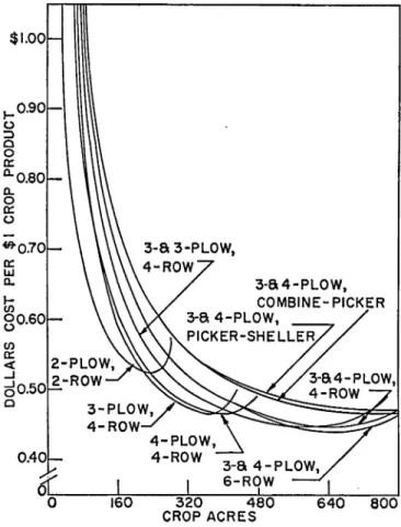
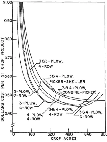
Since the cost curves of fig. 2 ignore crop losses resulting from untimeliness of operations, they do not answer the question of optimal farm size. Figure 3 in-cludes per-unit cost curves when losses from untimeliness Qf operations are considered. These are U-shaped, since per-unit costs increase as acreage is increased to suffi-cient magnitude for each machine combination. The curves turn upward, denoting that the acreage of minimum cost has been attained, when the losses from untimeliness more than offset the decline in average costs because of spreading fixed costs over a larger acreage.

. Generally, in economic textbooks, physical quantity is presented on the horizontal axis; dollar cost per unit qf physical output, on the vertical axis. The cost curves presented in fig. 3, however, do not measure cost against physical output. Aggregation of the individual products is necessary in determining average cost for a multiproduct firm. The most feasible and meaningful procedure is to aggregate the physical quantities by their respective prices. This procedure results in the measurement of costs per dollar of output, instead of costs per physical unit of output. The main disadvan-tage of this change in axis is that the cost schedules vary vertically with level of product prices.

A second difference between these cost curves and those typically included in economic textbooks deals with the quantity axis. In the cost curves presented here, the quantity measured on the horizontal axis is land input rather than output. The cost curves are presented in this mam~er to facilitate an~lysis ~nd inter-pretation of the data In terms of farm size. Since some

detail is lost in using land input rather than product

$1.00 1-0.90 o :J o o 0: c.. 0.80 c.. o 0: o fRo 0.70 0: LU c..

t;

Fig. 3. Average costs of producing $1 worth of crop product with eight machinery combinations based on current cropping methods.

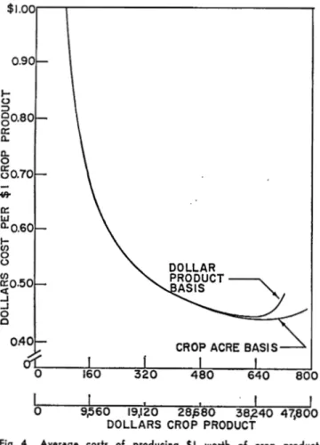
output on the horizontal axis, average per-unit costs are presented in fig. 4 for one set of machinery and one cropping system, with both land input and dollar of . output measured on the horizontal axis. The two average cost curves are identical at small acreages where crop losses resulting from untimely operations are negligible. With expanding acreage, crop losses gradually become more severe, and dollar output per acre declines. Hence, costs per dollar of output rise more sharply when measured against dollar output than when measured against acreage.

MINIMUM COST PER DOLLAR OF CROP OUTPUT RELATIVE TO ACREAGE

Minimum average costs for the 2-plow, 2-row com-bination are attained at 240 crop-acres, as shown in fig. 3. Below 200, and above 240 acres, average costs rise quite sharply for this machine combination. Farmers with 210 crop-acres or less would minimize per-unit costs by using this set of machinery. (The 2-plow, 2-row combination includes a complete line of field equipment except for crop-harvesting machines.)

The 3-plow, 4-row combination includes a complete complement of machinery for a 3-plow tractor. Of the machinery combinations studied, this set gives lowest average per-unit costs on acreages ranging from 210 to 370 crop-acres. The results illustrated in fig. 3 indi-cate that it would be unwise for a farmer with the

$ 1 . 0 0 . - - . - - - . . . . , . I-o :J 0.90 gO.80 a: ll. ll. o 50.70

*

o

DOLLARS CROP PRODUCT

Fig. 4. Average costs of producing $1 worth of crop product with crop-acres and total dollars product on the quantity axis (3- and 4-plow, 6-row machinery combination).

2-plow, 2-row combination to expand acreage to the point where average per-unit costs are a minimum. If

this farmer is operating 210 or more acres of cropland, he would be wise to, increase machinery investment instead of land investment. Between 200 and 280 crop-acres, untimeliness losses increas!,! rapidly with the 2-plow, 2-row machine combination. At 240 acres (the minimum average cost acreage for the 2-plow combina-tion), a shift to the 3-plow, 4-row combination would increase total annual costs by $68 but would increase total value product by $241.

The 4-plow, 4-row machinery combination includes the same machine items as the 3-plow, 4-row combina-tion except for a 4-plow tractor and a 4-bottom plow in place of a 3-plow combination. On farms with less than 370 crop-acres, per-unit costs are higher with the 4':plow than with the 3-plow combination. This is be-cause fixed costs are higher, and the additional field capacity with a 4-plow combination is not needed at these acreages. With 370 to 430 crop-acres, average per-unit costs are less with the 4-plow combination since severe untimeliness losses are avoided with the equipment of larger capacity.

All remaining machine combinations studied include two tractors and 4- or 6-row corn equipment. The 3-and 3-plow, 4-row combination includes two 3-plow tractors, 4-row corn equipment and a 2-row mounted corn picker. With this set of machinery, average costs are minimized at 640 acres. On a unit-cost basis, this 450

is the optimal set of machinery for farms ranging from 430 to 560 crop-acres. As with the 2-plow, 2-row com-bination, it would not be profitable to operate at the acreage which gives minimum per-unit costs with this set of machinery. Other sets of machinery give lower per-unit costs at 640 acres than are attained with this combination.

The 3- and 4-plow, 4-row machinery combination does not give lowest per-unit costs at any acreage. This set of machinery includes one 3-plow and one 4-plow tractor and 4-row corn equipment. Per-unit costs are lower with this combination than with the 3- and 3-plow combination on farms with 600 or more crop-acres. However, average per-unit costs are still lower with the machinery combination which includes 6-row corn equipment. The combination which includes 6-row equipment has nearly the same fixed costs as the 3-and 4-plow combination. Since it has a larger corn cultivating capacity, it results in lower untimeliness losses and, hence, in lower average costs per dollar of output.

Two sets of machinery also were studied which in-clude equipment for field shelling of corn. The com-bine-picker combination includes a 12-foot, self-propel-led combine-harvester with a corn-picker head, while the picker-sheller combination has a 12-foot, pull-type combine and a 2-row mounted corn picker with sheller attachment. Fixed costs are nearly the same for these two machinery sets. Calculated unit costs are slightly higher with the picker-sheller combination, however, because of higher repair costs per acre and slightly greater losses in oats harvesting. The minimum unit costs attainable with either of these two sets of machin-ery is higher than the minimum per-unit cost attainable with machinery sets which do not include field shellers. With field shellers, corn harvesting is estimated to begin 26 days earlier, thus greatly reducing corn har-vesting losses and also leaving more time for fall disking and plowing. Without field shellers, much less plowing or diskirig can be done in the fall, resulting in more planting untimeliness in the spring and in a definite limit to farm size. These savings in harvesting and planting losses are outweighed, however, by the 10-cent-per-bushel drying charge required for field-shelled corn.

As a result, minimum per-unit costs are estimated to be about 3 cents per dollar higher than with combinations which have conventional harvesting equipment. Actual-ly, drying of corn may be required in some years with conventional harvesting methods. Hence, the difference in minimum per-unit costs is probably less than 3 cents. This is a relatively small difference, and experienced operators may use picker-shellers or combine-pickers to gain a cost advantage, based on added value of product. Too, they may be able to get harvesting out of the way sooner and spend their time profitably on livestock. Certain of these results are summarized in table 3. With current cropping systems, large acreages are need-ed to obtain cost benefits from recent machinery inno-vations such as large-scale equipment and field shelling of corn. Also, the cost advantages to be gained are quite small. (The cost estimates in table 3 do not in-clude a charge for land or management and, hence, do not attempt to estimate total costs as a suggestion of profit per acre.)

Table 3. Costs per dollar product for all machinery combinations with current cropping systems and 1953·57 prices.

Machinery combination Range in acreage with lowest average total costs

t

!:~!~::

t::::::::::::::::::::::::::::::::

6. 3-and 4-plow, 6-row ...•.. _ .. _ ... _.

7. 3-and 4-plow, combine-picker ...• B. 3- and 4.plow, picker·sheller .•. _ .. _

0·210 210.370 370-430 430·560 none 560·800 800·960 nOlle Minimum average Minimum cost average acreage cost 240 360 400 640 680 680 760 760 $0.52 0.47 0.46 0.45 0.45 OM 0.47 0.47

From the data in table 3 and fig. 3, it appears that a machinery combination including one 4-plow tractor and 4-row com equipment allows attainment of most cost economies from expanded farm size. With this set of machinery, 400 crop-acres results in minimum costs per dollar of product. Six-row equipment gives lower per-unit costs only if farm size is expanded to 560 crop-acres. Although the possibility of using 6-row equipment with a I-tractor combination was not examined, such a possibility would not appear to be profitable. The budgeting of timeliness of field op~ra­ tions indicated that with the 4-plow, 4-row combma-tion, most of the untimeliness losses stem from delays in fall and spring disking and plowing. The extra com planting and cultivating capacity p~sible. with 6-r.ow equipment would be worth very httle m reducmg losses. The budgeting procedures indicated that some balance is needed in expanding machinery capacity. The expansion of field capacity in only one direction -for example, com cultivating - may not be profitable since other operations may provide the real bottleneck to profitable expansion of farm size.

Use of 4-row com equipment is estimated to result in cost savings of about 10 percent as compared with 2-row equipment (with comparison. at the acreage of minimum cost for each). This difference may cause pressure toward larger farms. Further expansion in machinery capacity to include 6-row equipment would reduce per-unit costs by an additional 1 or 2 cents per dollar of product. Acreage would have to be increased accordingly. This cost reduction alone may not be suffi-cient to serve as a "pushing force" toward farm en-largement. For prices sufficiently above per-unit costs, however, the greater income generated from farm en-largement and a volume of output could be an im-portant "pulling force" in this direction.

Field-shelling equipment alone does not give cost economies sufficiently great to induce greater farm size. Per-unit costs are generally higher with field shellers than with conventional harvesting equipment, even on larger farms. Here again, however, with sufficiently high product prices, the large volume that can be produced with combinations which include field shellers may favor the larger farm.

Results of this analysis indicate that, for any size farm, investment in machinery solely to eliminate all untimeliness losses is not profitable. For example, with 160 crop-acres, crop losses in all years are estimated to be zero only with the machi!l:ry combination.s w~ich

include field com shellers. WIth these combmatlOns, average costs per dollar of product are 4 cents above the next best combinations and 18 cents above the

least-cost set of machinery for a unit of 160 acres. Similar results are indicated at other acreages.

A farmer with a given set of machinery should expand the size of his farm beyond the point where no losses from untimely operations would occur. If, in so doing, he incurs small untimeliness losses which are more than offset by reduction in fixed costs per unit of output, profits will be increased. At some level of acreage per machine, however, the marginal losses from untimeliness become greater than the marginal cost of machinery for these purposes.

PER-UNIT COST FUNCTIONS

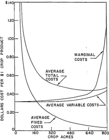
Regardless of the set of machinery under considera-tion, the structure of per-unit costs is similar. Figure 5 presents the various cost functions for the 3- and 4-plow, 6-row machinery combination. Results are similar for other sets of machinery; only the scales of measure-ment differ.

Average fixed costs per unit of output continue to decline as long as output increases. Average variable costs are almost constant for small acreages and increase slowly with increasing acreage. (Variable inputs per acre are nearly constant regardless of acreage. With in-creasing acreage, the only additional charges are for extra wear and tear on machinery.) The rise in the variable cost curve is due to the decrease in yields which results from untimely field operations as acreage grows sufficiently for a particular machine combination. This rise in variable costs per unit of output also is

char-$ 1 . 4 0 , , . . . - r r - - - , 1.20 I-(.) ;::) 0 0 a:

MARGIN~

*

AVERAGE VARIABLE

COST~

0 en cr ct ..J _0.20 ...J 0 0 0 0 160 800

Fig. 5. Per-unit cost functions for the 3- and 4-plow, 6-row machinery combination based on current cropping methods.

acterized in the marginal cost function. A marginal cost function of the shape shown in fig. 5 results for all of the machinery combinations studied. The marginal cost function "turns up" sharply where further expan-sion of farm size results in large losses from untimely operations. With current cropping systems, this increase in losses occurs especially at the acreage where corn planting interferes with soybean planting, resulting in very heavy losses in soybean production or vice versa. The average total cost curves for all two-tractor combinations are quite flat near the minimum-cost point. 7 _{For example, with the 3- and 4-plow, 6-row}

combinations, per-unit costs vary less than 5 cents per dollar of product between 400 and 840 crop-acres. With two-tractor combinations, losses from untimely opera-tions increase quite slowly over a wide acreage range. In this same acreage range, fixed costs per unit of output decline only slowly. For example, with a total fixed cost of $10 per acre, per-unit fixed cost is cut by 50 cents per acre as acreage is extended from 10 to 20. For this same total fixed cost, ho.wever, per-acre fixed cost declines by only 1

Y4

LONG-RUN FUNCTION

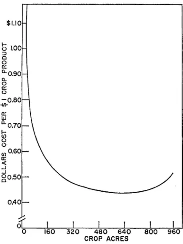
A long-run average cost curve, or envelope curve, is presented in fig. 6. This envelope curve is based on the eight sets of machinery discussed earlier and on current cropping techniques; the curve also is based on an approximation of the relevant points, selected from the separate short-run curves. As indicated in fig. 6, the acreage of minimum per-unit cost for the long-run curve is approximately 680 crop-acres. With free resource mobility, and with the resource prices assumed in this study, a farm of 680 acres could survive at the lowest product prices. Yet, average total costs vary less than 2 cents per dollar of product between 400 and 800 crop-acres. This small difference in per-unit costs over a wide acreage range would allow sur-vival of farms of many sizes at about the same price level. .

Per-unit costs increase quite sharply for acreages of less than 320 crop-acres. Cost economies are relatively large as acreage is extended to 320 acres.

The envelope curve also indicates rapidly increasing per-unit costs at farm sizes above 800 crop-acres. The long-run or envelope curve refers not to a single machinery combination but to all possible machine combinations. It shows the lowest cost, at any particular acreage, for the most economical machine combination.

RELATIONSHIP OF COST FUNCTIONS

TO CROPPING SYSTEM

The cost curves presented in the previous section only apply to a situation which meets the following specifications: Soil association area is Carrington-Clyde; cropping system includes current methods; fertilization

7 In this section the term "average total cost" is used to indicate the

sum of the vari~ble and fixed costs. It is not inferred that all costs have been considered. 452 $1.10

t;

"*

to

Fig 6. Long-run average cost or envelope curve based on cur-rent cropping methods and 1953-57 prices.

is at current levels; product prices are at 1953-57 average; input prices are at current mark~t rates; .and weather is "average." In this and followmg sectIOns, cost functions are estimated when these restricting con-ditions are relaxed in a singular fashion. Costs are estimated under two additional cropping systems and two fertilizer levels.

Costs Under a 5-Year Rotation Program

Cost curves are presented in this section for the eight sets of machinery (explained previously) used with a 5-year crop plan. This crop pattern includes 1 year of oats, 1 year of meadow, 2 years of corn and 1 year of half corn and half soybeans. Sixty percent of the cropland is in row crops. The first set of cost curves, presented in fig. 7, is based on current fertilization rates

Table 4. Comparisons of minimum per-unit costs with current cropping systems and a S-year rotation for six machin-ery combinations.

Minimum average costa Current

Machinery

combination cropping system rotation 5-yesr 2-plow, 2-row "'."."."_".'" $0.52

3-plow, 4-row '".''.''''''''''''''' 0.47 4-plow, 4-row ... _... 0.46 3- and 3-plow, 4-row ... _... 0,45

3-and 4-plow, 6-row ... 0.44 3- and 4-plow} combine-picker ... 0,47 $0.52 0.46 0.46 0.45 0.44 0.47

Minimum cost acreage

Current cropping 5-yesr system rotation 240 360 400 640 680 760 200 320 360 560 600 720 • Minimum average cost of producing $1 worth of crop product with 1953-57 average product prices.

$ 1 . 0 0 r - r " " I I T T - - - , 0.90

t;

/L

Fig. 7. Average costs of producing $1 worth of crop product with eight machinery combinations based on the 5-year rotation.

and 1953-57 prices. The relative cost relationships among machinery combinations are almost identical to results obtained for the current cropping system.

Table 4 summarizes relevant cost and acreage data for both a 5-year rotation plan and current cropping methods. The main effect of the change in cropping system is a reduction in the number of acres to provide a cost minimum (i.e., the acreage associated with the low point on the cost curve). For example, the acreage associated with the acreage of cost minimum declines from 240 to 200 acres for the 2-plow, 2-row machinery combination and from 360 to 320 acres with the 3-plow, 4-row combination. With more intensive use of row crops, labor and other input requirements per acre are increased. Yields per acre also are increased. Thus, the size of farm necessary to give minimum costs is reduced. Minimum per-unit costs with the 5-year rotation are almost identical to those estimated for current cropping systems. Profit from total inputs is greater under the former system, however, because land investment is smaller.

As suggested in fig. 7, the main cost advantages of different crop acreages and machine combinations is attained by the time acreage is expanded to around 300 acres. As indicated in table 4, the minimum cost with a 3-plow, 4-row combination is attained at 320 acres. Other combinations give slightly lower costs at larger acreages. However, the extremely large reduc-tions in per-unit costs have been attained at 300 acres even by the 3-plow, 4-row combination. Cost savings

per dollar of crop product alone are not great enough, beyond this acreage, to result in extreme pressure to-ward larger farms. Actually, the larger acreages and bigger machine combinations do little more than dup-licate the level of per-unit costs attained at 300 crop-acres by the 3-plow, 4-row combination. Too, remem-ber that all labor (operator, family and hired) is charged as an expense or cost in these calculations. The larger units would need to use some hired labor, while farms of smaller acreages would not. Hence, with lower cost for some family labor, the actual out-of-pocket cost would generally be as low with 300-320 crop-acres and a 3-plow, 4-row combination as at 600 acres with two 3-plow tractors and 4-row equipment. This same gen-eral conclusion would apply to other cost combina-tions which follow. Under both cropping systems, cost advantages for combinations including two tractors are small.

Effect of Fertilizer Application Level on

Per-Unit Costs for Carrington-Clyde Soils

The cost curves presented thus far are based on fer-tilization rates representing an average of those used in the Carrington-Clyde soil area at the time of the study. These rates approximated an 8-20-20 (pounds of active ingredients of N, P205 and K20 per acre)

mixture on corn and a 0-20-0 mixture on oats. Cost curves presented in this section, for three sets of ma-chinery only, are based on a higher fertilization rate. Yields are increased accordingly and amount to 7 bushels for corn, with proportional increases in the yields of other crops.

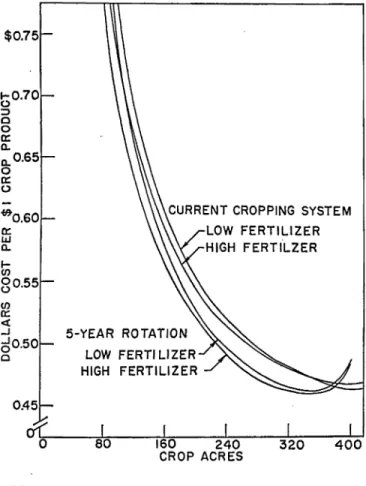
Figures 8, 9 and 10 include the resulting per-unit cost curves, with land charges excluded, for two crop-ping systems and two fertilizer levels with three sets of machinery. The shape of the cost curve is affected relatively little by a change in the rate of fertilizer application. The slope, particularly on the upward sloping portion of the curve, is especially determined by losses from untimely field operations. Since untime-liness losses are determined largely by the same acre-ages against a given set of machinery, the shape of the cost curves remains nearly the same regardless of the f ertili ty level.

Under high fertilization, per-unit costs of crop output are generally lower than under the lower fertilization rates. In absolute amounts, the total value of product increases considerably more than does cost of fertilizer application. The optimal amount of ferti-lizer input is, of course, best determined by marginal analysis, rather than by comparison of farm cost func-tions. With the 5-year rotation, use of the high ferti-lizer level increases costs of fertiferti-lizer by $2.95 per acre but increases value product, with no untimeliness losses, by $7.51 per acre at 1953-57 prices. The opti-mum fertilizer level is represented by a rate at which marginal return is equal to marginal cost. Return and cost levels depend, of course, on the price of fertilizer and the prices of the products. Marginal value return, for the rates indicated, is double the cost of the addi-tional fertilizer even at product prices as low as those which existed in 1958.

$0.80 0.75

b

CURRENT CROPPING SYSTEM LOW FERTILIZER HIGH FERTILIZER 5·YEAR ROTATION LOW FERTILIZER HIGH FERTILIZER 400

Fig. 8. Average costs of producing $1 worth of crop product with the 2.plow, 2-row machinery combination for two cropping systems and two fertilizer levels.

$0.75

5

CURRENT CROPPING SYSTEM LOW FERTILIZER HIGH FERTILZER

5-YEAR ROTATION LOW FERT! UZER HIGH FERTILIZER $0.7 t;0.70 :J a o a:: 0-0. 0.65 o a:: (.) ~0.60 a:: 1IJ 0.

t;

«

Fig. 9. Average costs of producing $1 worth of crop product with the 4.plow, 4-row machinery combination for two cropping systems and two fertilizer levels.

Fig. 10. Average cost of producing $1 worth of crop product with the 3. and 4-plow, 6-row machinery combination for two cropping systems and two fertilizer levels.

Per-Unit Costs Under a Continuous-Corn

Program on Carringto.n-Cly,de Soils

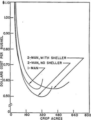
Cost functions are developed in this section for a continuous-corn cropping program on Carrington-Clyde soils. Somewhat different machinery combina-tions are required since hay harvesting is eliminated. Three such sets of machinery, all inCluding 6-row corn equipment, have been used for these calculations. The first set is designed for operation by one man. It in-cludes a 4-plow tractor, 6-row corn equipment and a 2-row mounted picker with sheller attachment. A second set, designed for operation by two men; in-cludes one 4-plow and one 3-plow tractor, 6-row and 4-row corn equipment and a 2-row mounted corn picker. A third set, also for operation by two men; is . a duplicate of the second set with the addition of a sheller attachment on the corn picker. Only one plow would be needed with the 2-tractor combinations; the second tractor would be used for other operations such as disking; harrowing and planting.

A corn yield of 71 bushels per acre is assumed with continuous corn, with total fertilizer input of $9.77 per acre per year. The resulting average cost curves for the three sets' of machinery on Carrington-Clyde soils are presented in fig. 11. The vertical axis is cost per bushel of corn, rather than costs per dollar of product; since aggregation of products is not neces-sary. Under the continuous-corn program, the one-man operation gives lowest per-unit costs only on farms of less than 96 crop-acres. At 96 acres, average costs per unit of output still are declining quite rapidly, indicating that such small farms would be uneco-nomical.

The two-man or 2-tractor operation without a field sheller attachment gives lowest per-unit costs for farm units over a range of approximately 100 to 400 acres. The two-man operation with a picker-sheller has lower unit costs for more than 400 acres.

Table 5 provides a comparison of certain cost and acreage quantities for the continuous-corn and 5-year rotation systems. Both cropping programs are based on the same general level of fertilization, adjusted for the rotations and the same price levels. Per-unit production costs with the continuous-corn program are expressed in costs per dollar product to facilitate comparison. (The price of corn used is $1.30 per bushel.) Again, the acreage at which costs are at a minimum is smaller under continuous corn than under the rotation. The major per-unit cost gains are attained at 240 crop-acres with the continuous-corn program. The comparable size is 320 acres under the 5-year rotation and 400 acres under current cropping programs.

The structure of fixed and variable costs differs considerably between the continuous-corn and the other two cropping programs. Total machinery investment is considerably lower with machinery combinations for the continuous-corn program. Fixed machinery costs per acre, at the acreages of minimum cost; average slighly higher with continuous com since optimal farm size is smaller. However; variable machinery costs per dollar of output are lower. Average costs (the sum of fixed and variable costs per unit) per $1 of output are; in total; slightly less for continuous corn; mainly

$ 1 . I O I r - l r r - - - , .J III :I: UJ : l 1.00 0.90 IIlO.SO

ffi

Iii

Fig. II. Averoge costs of producing corn with a continuous-corn cropping system.

Table 5. Minimum per-unit costs of producing $1 worth of crop product with the continuous-corn program and the 5· yeor rotation on Corrington-Clyde soils.

Machinery combination Continuous-com Acreage of minimum cost One-man •...•.. _ ... _ .. _ ... _... 280

Two-man (no sheller) ... _ ...•.. _... 320

Two-man (sheller) ... _... 440 5-year rotation

4- plow, 4-row ... _ .. _ .. _ ... _... 360 3- and 4-p!ow, 6-row ... _ ... _... 600 3- and 4-p!ow, picker-sheller ... ,. i20

Minimum cost per dollar of product $0.42 0.39 0.43 0.46 0.44-0.47

because of the larger value of output per acre. Corn produces a greater value product per acre than do oats; hay and soybeans.

COMPARISON OF COST FUNCTIONS

FOR TWO SOIL TYPES

This section deals with cost functions for Ida-Monona soils. While these soils are relatively fertile, the topography differs greatly from that of the Car-rington-Clyde area. Only 20 percent of the farmland in the Ida-Monona area has a slope of 4 percent or less, and 22 percent has a slope of 14 percent or more. Under these conditions; terraces, contouring and other conservation practices must be used if soil erosion is to be controlled and yields are to be maintained. Topography also limits the selection of rotations and