Abstract
The Grid has the potential to grow significantly over the course of the next decade and therefore the mechanisms that make the Grid possible need to become more efficient in order for the Grid to scale. One of these mechanisms revolves around resource management; ultimately, there will be so many resources in the Grid, that if they are not managed properly, only a very small fraction of those resources will be utilized. While good resource utilization is very important, it is also a hard problem due to widely distributed dynamic environments normally found in the Grid. It is important to develop an experimental methodology for automatically characterizing grid software in a manner that allows accurate evaluation of the software’s behavior and performance before deployment in order to make better informed resource management decisions. Many Grid services and software are designed and characterized today largely based on the designer’s intuition and on ad hoc experimentation; having the capability to automatically map complex, multi-dimensional requirements and performance data among resource providers and consumers is a necessary step to ensure consistent good resource utilization in the Grid. This automatic matching between the software characterization and a set of raw or logical resources is a much needed functionality that is currently lacking in today’s Grid resource management infrastructure. Ultimately, my proposed work, which addresses performance modeling with the goal to improve resource management, could ensure that the efficiency of the resource utilization in the Grid will remain high as the size of the Grid grows.
1.0 Introduction
Through my previous work, I have shown that DiPerF [1, 2, 3] can be used to model the performance characteristics of a service in a client/server scenario. Using the basic concept of DiPerF, I believe I can also create performance models that can be used to predict the future performance of distributed applications. Modeling distributed applications (i.e. parallel computational programs) might be more challenging since the dataset on which the applications work against often influence the performance of the application, and therefore general predictive models might not be sufficient.
Using DiPerF and a small dedicated cluster of machines, we can build dynamic performance models to automatically map raw hardware resources to the performance of a particular distributed application and its representative workload; in essence, these dynamic performance models can be thought of as job profiles, and will be implemented in the component DiProfile. The intuition behind DiProfile is that based on some small sample workload (with varying sizes) and a small set of resources (with varying size), we can make predictions regarding the execution time and resource utilization of the entire job running over the complete dataset. The DiProfile stage will be a relatively expensive component in both time and computational resources, however its overhead will be warranted as long as the typical job submitted is significantly larger than the amount of time DiProfile needs to build its dynamic performance models.
There is a gap between software requirements (high level) and hardware resources (low level). Automatic mapping could produce better scheduling decisions and give users feedback with the expected running time of their software. Using DiProfile, we can make predictions on the performance of the jobs based on the amount of raw resources dedicated to the jobs. The accuracy of the predictions will heavily rely on the idea that reliable software performance characterization is possible with only a fraction of the data input space.
Using DiPred and user feedback (or even user specified high level performance goals), the scheduler (DiSched) can make better decisions to satisfy the requested duration of the job, where the job should be placed, etc. Since jobs are
Ioan Raicu
Department of Computer Science
University of Chicago
1100 E. 58th Street, Ryerson Hall
Chicago, IL 60637
profiled based on what raw resources they will likely consume and the duration of those resource usage, multiple different jobs could be simultaneously submitted to the same nodes without any significant loss of individual job performance; this would certainly increase resource utilization and as long as the predicted resource usage does not exceed the available resources, the time it takes to complete individual jobs should not be significantly affected. The increase of resource utilization is possible as long as the assumption that several different classes of software can be concurrently executed without significant loss of performance.
It is expected that Resource Managers could use a combination of resource selection algorithms besides the proposed DiSched component. To ensure that the available resources that the scheduler is aware of is maintained and updated, resource monitoring (i.e. Ganglia, MDS, etc…) will also be necessary. Some current resource managers use resource monitoring to make scheduling decisions, but often only one job is normally submitted to each individual resource. However, combining resource monitoring with predictive scheduling has the potential to not only improve scheduling decisions to yield lower end-to-end job execution times, but to increase resource utilization significantly.
2.0 Related Work
The goals of mapping software requirements to available resources has been studied extensively, however, in practice, it is still a relatively manual process and is application specific. One approach is to perform benchmarks on resources, however this still requires user specified relationships between benchmarks and software requirements to be established. Performing these benchmarks on the resources acts as a “stepping stone” towards gaining insight about the performance of a particular set of resources, and what kind of problems could possibly benefit the most from them. Regarding application performance models, there seems to be two general methods, workflow analysis and the use of compilers to some degree. The drawbacks of workflow analysis is that it is a hard problem and time consuming to produce accurate workflows. As for compiler technology, it requires user intervention to model complex applications. Furthermore, performance models might not reflect actual performance on various different architectures.
What I propose is to seek an automatic mapping between software requirements and available resources using “black box” approach, which would be ideally generic and application independent. In principle, performance models could be built to be classified into several software classes based on the type and amount of resource usage. The models would take into consideration interactions between various components in the system, and across distributed and different systems. Best of all, applications could have performance models built without any modifications or expert knowledge about the particular software.
Some of the lessons learned from the related work are that benchmarking of Grid resources could be used to enhance the resource selection, especially in the heterogeneous systems that are often found in today’s Grids. Co-scheduling could also be used based on the software classes established to increase the resource utilization. Furthermore, historical information could be used to recall the performance models generated for commonly used software in order to save the cost of generating a new model. Much of the surveyed work concentrated on lower levels of scheduling (i.e. local scheduling); it is important to address scheduling decisions on a larger global scale, and perhaps giving hints to the low level schedulers in order to improve the low level local scheduling.
2.1 Benchmarking of Resources
GridBench [30, 31] is a set of tools that aim to facilitate the characterization of Grid nodes or collections of Grid resources. In order to perform benchmarking measurements in an organized and flexible way, we provide the GridBench framework as a means for running benchmarks on Grid environments as well as collecting, archiving, and publishing the results. This data is available for retrieval not only by end users, but also for automated decision-makers such as schedulers. A scheduler could use micro-benchmark results to “rank” the resources based on performance (CPU, memory or MPI). Additionally, a scheduler could evaluate a resource's “health” by invoking one of the micro-benchmarks. Since execution times are typically less than 10 seconds, this would impose little additional delay and would potentially save a scheduler from time-consuming failed submissions. Once the relationship between the micro-benchmarks and the application kernel has been established (in a manual fashion that involves human intervention and detailed knowledge of the application or its empirical performance) it can then be applied to resource selection.
Elmroth et al [38] presents algorithms, methods, and software for a Grid resource manager, responsible for resource brokering and scheduling in early production Grids. The broker selects computing resources based on actual job requirements and a number of criteria identifying the available resources, with the aim to minimize the total time to
delivery for the individual application. The total time to delivery includes the time for program execution, batch queue waiting, input/output data transfer, and executable staging. Main features of the resource manager include advance reservations, resource selection based on computer benchmark results and network performance predictions, and a basic adaptation facility. The performance differences between Grid resources and the fact that their relative performance characteristics may vary for different types of applications makes resource selection difficult. Our approach to handle this is to use a benchmark-based procedure for resource selection. Based on the user’s identification of relevant benchmarks and an estimated execution time on some specified resource, the broker estimates the execution time for all resources of interest. The authors assume linear scaling of the application in relation to the benchmark, i.e., a resource with a benchmark result a factor k better is assumed to execute the application a factor k faster. For each of these benchmarks, the user needs to specify a benchmark result and an expected execution time on a system corresponding to that benchmark result. The time estimation for the stage in and stage out procedures are based on the actual (known) sizes of input files and the executable file, user-provided estimates for the sizes of the output files, and network bandwidth predictions. The network bandwidth predictions are performed using the Network Weather Service (NWS) [42]. NWS combines periodic bandwidth measurements with statistical methods to make short-term predictions about the available bandwidth.
2.2 Workflow Analysis
Spooner et al. [32] developed a multi-tiered scheduling architecture (TITAN) that employs a performance prediction system (PACE) and task distribution brokers to meet user-defined deadlines and improve resource usage efficiency. This work focused on the lowest tier which is responsible for local scheduling. By coupling application performance data with scheduling heuristics, the architecture is able to balance the processes of minimizing run-to-completion time and processor idle time, whilst adhering to service deadlines on a per-task basis. The PACE system provides a method to predict the execution time dynamically, given an application model and suitable hardware descriptions. The hardware (resource) descriptions are generated when the resources are configured for use by TITAN, and the application models are generated prior to submission. PACE models are modular, consisting of application, sub-task, parallel and resource objects. Application tools are provided that take C source code and generate sub-tasks that capture the serial components of the code by control flow graphs. It may be necessary to add loop and conditional probabilities to the sub-tasks where data cannot be identified via static analysis. The parallel object is developed to describe the parallel operation of the application. This can be reasonably straightforward for simple codes, and a library of templates exists for standard constructs. Applications that exhibit more complex parallel operations may require customization. The sub-tasks and parallel objects are compiled from a performance specification language (PSL) and are linked together with an application object that represents the entry point of the model. Resource tools are available to characterize the resource hardware through micro-benchmarking and modeling techniques for communication and memory hierarchies. The resultant resource objects are then used as inputs to an evaluation engine which takes the resource objects and parameters to produce predictive traces and an estimated execution time. Scheduling issues are addressed at this level using task scheduling algorithms driven by PACE performance predictions. In summary, the techniques presented have been developed into a working system for scheduling parallel tasks over a heterogeneous network of resources. The Genetic Algorithm forms the centre point of the localized workload managers and is responsible for selecting, creating and evaluating new schedules. Prophesy [40] is an infrastructure for performance analysis and modeling of parallel and distributed applications. Prophesy includes three components: automatic instrumentation of applications, databases for archival of information, and automatic development of performance models using different techniques. The default mode consists of instrumenting the entire code via PAIDE at the level of loops and procedures. PAIDE includes a parser that identifies where to insert instrumentation code. PAIDE also generates two files: (1) the call graph of the application and (2) the locations in the code where instrumentation was inserted. The information in these two files allows the performance data to be directly related to the application code for code tuning. A user can specify that the code be instrumented at different levels of granularity or manually insert directives for the instrumenting tool to instrument specific segments of code. The resultant performance data is automatically placed in the performance database. This data is used by the data analysis component to produce an analytical performance model at the level of granularity specified by the user, or answer queries about the best implementation of a given function. The models are developed based upon performance data from the performance database, model templates from the template database, and system characteristics from the systems database. These models can be used to predict the performance of the application under different system configurations. Currently, Prophesy includes three methods for developing analytical models for predictions: (1) curve fitting, (2) parameterized model of the application code, (3) coupling of the kernel models. The advantage of curve fitting is the ease for which the analytical model is
generated; the disadvantage is the lack of exposure of system terms versus application terms. Hence, models resulting from curve fitting can be used to explore application scalability but not different system configurations. Parameterization is a method that combines manual analysis of the code with system performance measurements. The manual analysis entails hand-counting the number of different operations in the code. Having the system and application terms represented explicitly, one can use the resultant models to explore what happens under different system configurations as well as application sizes. The disadvantage of this method is the time required for manual analysis. Kernel coupling refers to the effect that kernel i has on kernel j in relation to running each kernel in isolation. The two kernels can correspond to adjacent kernels in the control flow of the application or a chain of three or more kernels. The coupling value provided insight into where further algorithm and code implementation work was needed to improve performance, in particular the reuse of data between kernels.
Pegasus [43, 44] (Planning for Execution in Grids) was developed at ISI as part of the GriPhyN and SCEC/IT projects. Pegasus is a configurable system that can map and execute complex workflows on the Grid. Currently, Pegasus relies on a full-ahead-planning to map the workflows. The main difference between Pegasus and other work on workflow management is that while most of the other system focus on resource brokerage and scheduling strategies while Pegasus uses the concept of virtual data and provenance to generate and reduce the workflow based on data products which have already been computed earlier. It prunes the workflow based on the assumption that it is always more costly the compute the data product than to fetch it from an existing location. Pegasus also automates the job of replica selection so that the user does not have to specify the location of the input data files. Pegasus can also map and schedule only portions of the workflow at a time, using just in-time planning techniques. Although Pegasus provides a feasible solution, it is not necessarily a low cost one in term of performance.
Jang et al [33] presents a resource planner system consisting of the Pegasus [43, 44] workflow management and mapping system combined with the Prophesy [40] performance modeling infrastructure. Pegasus is used to map an abstract workflow description onto the available grid resources. The abstract workflow indicates the logical transformations that need to be performed, their order and the logical data file that they consume and produce. The abstract workflow does not include information about where to execute the transformations nor where the data is located. Pegasus uses various grid services to find the available resources, the needed data and the executables that correspond to the transformations. Pegasus also reduces the abstract workflow if the intermediate products are found to already exist somewhere in the grid environment. One of the ways that Pegasus maps a workflow onto the available resources is through random allocation. This work interfaces Pegasus and Prophesy to enable Pegasus to use the Prophesy prediction mechanisms to make more informed resources choices.
The goal of the Grid Application Development Software Project (GrADS) [28] is to realize a Grid system, by providing tools, such as problem solving environments, Grid compilers, schedulers, performance monitors, to manage all the stages of application development and execution. Using GrADS the user will only concentrate on high-level application design without putting attention to the peculiarities of the Grid computing platform used. The GrADS system is composed of three main components: Program Preparation System (PPS), Configurable Object Program (COP), and Program Execution System (PES). The PPS component handles application development, composition, and compilation. To develop their Grid application, users interact with a high-level interface providing a problem solving environment, which permits the integration of the application source code, software components and library modules. Then, the resulting application is passed to a specialized GrADS compiler that generates an intermediate representation code and a configurable object program (COP). The COP encapsulates all results (e.g. application performance models and the intermediate application representation code) of the PPS phase for later usage. The PES components provides on-line resource discovery, scheduling, binding, application performance monitoring, and rescheduling. To execute an application, the user submits parameters of the problem such as problem size to the GrADS system. The PPE component receives the COP as input and, at this stage, the scheduler carries out an application-appropriate schedule. The binder is then invoked to perform a final, resource-specific compilation of the intermediate representation code. Next, the executable is launched on the selected Grid resources and a real-time performance monitor is used to track program performance and detect violation of performance guarantees. Performance guarantees are formalized in a performance contract. In the case of a performance contract violation, the rescheduler is invoked to evaluate alternative schedules. The scheduler is a key component of the GrADS system. In GrADS, scheduling decisions are taken by exploiting application characteristics and requirements in order to obtain the best application execution time.
Dail et al [37] proposed an application scheduling approach designed to improve the performance of parallel applications in Computational Grid environments. The approach is general and can be applied to a range of applications in a variety of execution environments. This flexibility is achieved through a decoupling of the
scheduler core (the search procedure) from the application-specific (e.g. application performance models) and platform-specific (e.g. collection of resource information) components used by the search procedure. While the scheduler can be used in a stand-alone fashion, it has been designed specifically for a larger program development environment such as the Grid Application Development Software (GrADS) project. The decoupled design allows integration with other GrADS components to provide transparent and generic scheduling. To provide application appropriate scheduling, the system depends on the availability of two application-specific components: a performance model and a mapper. As the GrADS system matures, the authors hope to obtain such components automatically from application development tools such as the GrADS compiler. The performance model is an analytic metric for the performance expected of the application on a given set of resources. The mapper provides directives for mapping logical application data or tasks to physical resources. To validate their approach in the absence of such facilities, they hand-built performance models and mappers for two applications: Game of Life and Jacobi. The performance of the various scheduling methods was: local MDS cache ~ 4.5 seconds; remote NWS nameserver ~ 62.4 seconds; remote NWS nameserver and remote MDS server ~ 1088.4 seconds. The authors assume that a Grid user will probably be willing to wait 60 seconds for scheduling, but will probably not be willing to wait 1000 seconds. These results indicate that, given the technologies available at the time of their experiments (2002), their scheduling approach is only feasible when used with a local MDS cache.
AppLeS (Application Level Scheduling) [45] is a project leaded by F. Berman at the University of California, S. Diego. It is a methodology for adaptive application scheduling on heterogeneous computing platforms. The AppLes approach exploits static and dynamic resource information, performance predictions, application and user-specific information, and scheduling techniques that adapt “on-the-fly” to application execution. In Figure 2 the phases in the Apples scheduling methodology are shown. As we can see, the System Selection phase of the general scheduler architecture of Figure 1, in AppLeS is split into three sub-phases: (2) Resource selection, (3) Schedule generation, and, (4) Schedule selection. During sub-phase (2) the resources enabled to run the application are selected according to application-specific resource selection models. To this end, AppLeS uses information carried out by the Network Weather Service (NWS) performance monitor (NWS is a distributed system that periodically monitors and dynamically forecasts the performance various network and computational resources can deliver over a given time interval). An ordered list of viable resources is finally produced. In (3) a performance model is applied to determine a set of candidate schedules for the application on the selected resources (for any given set of resources, many schedules may be possible). In (4) the schedule that best matches the chosen performance criteria is selected. The AppLeS approach requires to integrate in the application a scheduling agent which must be customized according to application features. In order to make easier this customization, templates to be applied to classes of applications with common characteristics were introduced. Templates for parameter sweep applications (APST), master/worker applications (AMWAT), and for scheduling moldable jobs on spaceshared parallel supercomputers (SA) are currently available.
2.3 Co-Scheduling
Frachtenberg et al. [34, 35] performed a detailed performance evaluation of 5 factors affecting scheduling systems running dynamic workloads: multiprogramming level, time quantum, gang scheduling, backfilling, and flexible co-scheduling [36]. The results demonstrated the importance of both components of the gang-co-scheduling plus backfilling combination: gang scheduling reduced response time and slowdown, and backfilling allowed doing so with a limited multiprogramming level. This was further improved by using flexible co-scheduling rather than strict gang scheduling, as this reduced the constraints and allowed for a denser packing. Multiprogramming on parallel machines may be done using two orthogonal mechanisms: time slicing and space slicing. With time slicing, each processor runs processes belonging to many different jobs concurrently, and switches between them. With space slicing, the processors are partitioned into groups that serve different jobs. Gang scheduling is a technique that combines the two approaches: all processors are time-slices in a coordinated manner, and in each time slot, they are partitioned among multiple jobs. Gang scheduling may be limited due to memory constraints. Backfilling is an optimization that improves the performance of pure space slicing by using small jobs from the end of the queue to fill in holes in the schedule, however to do so, it requires users to provide estimates of job run times. The flexible co-scheduling employs dynamic process classification and schedules processes using this class information. Processes are categorized into one of four classes: CS (coscheduling), F (frustrated), DC (don’t-care), and RE (rate-equivalent). CS processes communicate often, and must be coscheduled (gang-scheduled) across the machine to run effectively, due to their demanding synchronization requirements. F processes have enough synchronization requirements to be co-scheduled, but due to load imbalance, they often cannot make full use of their allotted CPU time. This load imbalance can result from any of the reasons detailed in the introduction. DC processes rarely
synchronize, and can be scheduled independently of each other without penalizing the system’s utilization or the job’s performance. For example, a job using a coarse-grained workpile model would be categorized as DC. RE processes are characterized by jobs that have little synchronization, but require a similar (balanced) amount of CPU time for all their processes. Processes are categorized based on measuring process statistics; this was achieved by implementing a lightweight monitoring layer that was integrated with MPI. Synchronous communication primitives in MPI call one of four low-latency functions to note when the process starts/ends a synchronous operation and when it enters and exits blocking mode. Applications only need to be re-linked with the modified MPI library, without any change. The accuracy of this monitoring layer has been verified using synthetic applications for which the measured parameters are known in advance, and found to be precise within 0.1%. In summary, batch and gang scheduling perform poorly under dynamic or load-imbalanced workloads, whereas implicit co-scheduling suffers from performance penalties for fine-grained synchronous jobs. Most job schedulers offer little adaptation to externally- and internally fragmented workloads, resulting in reduced machine utilization and response times. On the other hand, Flexible Co-Scheduling was designed specifically to alleviate these problems by dynamically adjusting scheduling to varying workload and application requirements.
2.4 Other
Liu et al [39] presents a general-purpose resource selection framework that addresses the problems of first discovering and then organizing resources to meet application requirements by defining a resource selection service for locating Grid resources that match application requirements. At the heart of this framework is a simple, but powerful, declarative language based on a technique called set matching, which extends the Condor matchmaking framework to support both single resource and multiple-resource selection. This framework also provides an open interface for loading application-specific mapping modules to personalize the resource selector. Within this framework, both application resource requirements and application performance models are specified declaratively, in the ClassAd language, while mapping strategies can be determined by user-supplied code. Liu et al [46] extended this work by designing and implementing a description language, RedLine, for expressing constraints associated with resource consumers (requests) and resource providers. They have also implemented a matchmaking process that uses constraint-solving techniques to solve the combinatorial satisfaction problems that arise when resolving constraints. The resulting system has significantly enhanced expressiveness compared with previous approaches, being able to deal with requests that involve multiple resources and that express constraints on policies as well as properties.
Some of the various methods used or proposed in the literature for extracting performance models are: • Genetic Algorithm [32, 41]
• Simulated Annealing [41] • Tabu Search [41]
• Curve fitting (least squares) [40] • Parameterization [40]
• Kernel coupling [40] • Time series analysis 3.0 Proposed Work
The proposed work is aimed at developing the following four components with the goals to increasing resource utilization while decreasing end-to-end job execution times using predictive scheduling in the Grid:
1. DiPerF – A Distributed Measurement Framework 2. DiProfile – A Job Profiler for distributed software
3. DiPredict – Performance Predictions of distributed computations
Gate
Keepers
JOB
Software Requirements: I don’t know...Output
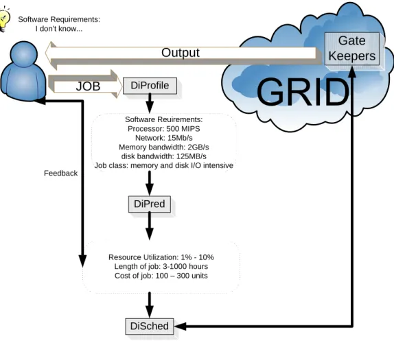
DiProfile DiSched DiPred Software Reuirements: Processor: 500 MIPS Network: 15Mb/s Memory bandwidth: 2GB/s disk bandwidth: 125MB/s Job class: memory and disk I/O intensiveResource Utilization: 1% - 10% Length of job: 3-1000 hours Cost of job: 100 – 300 units Feedback
Figure 1: Proposed system overview
DiPerF is included as one of the 4 components due to the fact that it already exists as it was part of my previous work, and it is the foundation of the DiProfile component. The DiProfile components will essentially be the DiPerF framework specialized for the task of profiling software in a fully automatic manner and outputting the needed results to the next component, namely DiPredict.
Figure 1 presents the proposed system overview. Note that the 3 components (DiProfile, DiPred, and DiSched) are placed in between the user and the Grid; the proposed system is meant to act as a run-time tool to aid in scheduling decisions. The DiProfile component breaks analyzes the software and its input and generates the needed hardware requirements and tries to classify the software class in which that particular software belongs to. The DiPredict component then attempts to use the hardware requirements and build some high level choices that the user could choose from, such as resource utilization desired, length of job desired, or maximum cost allowed. Based on the feedback or the user and the predictions made by DiPredict, the DiSched component can then perform a matchmaking between what the user wants, with the software requirements, and the available resources.
3.1 DiPerF: Collection of performance measurements in a distributed environment
There has been much work [4-10] in the area of performance measurements for both service performance in a distributed environment and network performance. An important aspect to understanding the performance of complex system that has not been addressed in the literature is the performance of individual clients (and the aggregate performance of many clients). To address this specific point, I have developed DiPerF [1], a scalable distributed performance testing framework that is aimed at simplifying and automating service performance evaluation. DiPerF’s overall objective is to collect the necessary performance metrics from a complex distributed system in order to quantify service performance, client performance, and communication infrastructure (i.e., network) performance. DiPerF coordinates a pool of machines that test a target service, collects and aggregates performance metrics, and generates performance statistics. The aggregate data collected provide information on service throughput, on service ‘fairness’ when serving multiple clients concurrently, and on the impact of network latency on service performance. DiPerF was designed to scale to 10,000s of concurrent clients with 100,000s of
transactions per second. The central hypothesis is that such a framework can be built and that the collected metrics can be combined to depict the aggregate client view. The expected outcome is a fully automated tool implemented over several testbeds (e.g., Grid3, PlanetLab, clusters) that tests service performance and provides detailed statistics about the network and the service performance from both the client and service view. The preliminary results obtained from two test cases (GRAM job submission in Globus Toolkit and web server performance) and another scalability study currently being investigated shows that the scalability goals of DiPerF are realizable and suggest that DiPerF provides a solid foundation for the proposed research. The expected significance of DiPerF is the ability to observe the client view, the service view, and the network performance with the goal that these three different views combined together can offer insight regarding the performance of a service that was not present in just one of the views.
3.2 DiProfile: Perform software characterization
Modeling distributed applications (i.e. parallel computational programs) might be more challenging since the dataset on which the applications work against often influence the performance of the application, and therefore general static predictive models might not be sufficient. Using DiPerF and a small dedicated cluster of machines, we can build dynamic performance models to automatically map raw hardware resources to the performance of a particular distributed application and its representative workload; in essence, these dynamic performance models can be thought of as job profiles, and will be implemented in the component DiProfile. The intuition behind DiProfile is that based on some small sample workload (with varying sizes) and a small set of resources (with varying size), we can make predictions regarding the execution time and resource utilization of the entire job running over the complete dataset. The DiProfile stage will be a relatively expensive component in both time and computational resources, however its overhead will be warranted as long as the typical job submitted is significantly larger than the amount of time DiProfile needs to build its dynamic performance models.
We envision that several different software classes will emerge which DiProfile will be able to automatically identify which class any software belongs to; these classes would probably represent the average case resource utilization for each respective metric. Some of these classes could be:
• CPU Intensive only • Network Intensive only
• Memory Intensive only (capacity) • Memory Intensive only (bandwidth) • Storage Intensive only (capacity) • Storage Intensive only (bandwidth) • Any combination of the above classes
The number of software classes could quickly grow due to the many combinations possible, however defining such software classes will have certain advantages especially in scalability at the sacrifice of some expressivity. One could imagine once some software is characterized and classified with a particular class, then defining rules to decide what other software could be co-scheduled concurrently could be easily realized.
The questions that remain unanswered for this section are:
1. Can the performance of a complex piece of software that heavily depends on its input be characterized in its entirety in a fraction of the time that it would take to run the entire workload?
2. Is the average case resource utilization sufficient to make the software class useful in real world resource management?
3. How flexible will the job profiler be to different types of software classes? 4. What is the maximum amount of time users are willing to wait for a job profile?
5. What overall performance improvement is needed in order to offset the extra complexity, time, and resources that the software profiler introduces?
3.3 DiPredict: Automatic mapping of software requirements to raw resources & Service Performance Predictions
Using the data generated by DiProfile, I believe it is possible to build analytical models that estimate a service performance given some characterization of the resources that would be utilized and the current state of those
resources. Previous research [11-19] has used statistical time series, regression and/or historical information in order to perform predictions in the context of service performance or network performance. On the other hand, there are other multivariate analytical models that have the potential of having better predicting accuracy. The Grid is a complex system, and often no particular metric is sufficiently comprehensive; however, an approach (such as neural networks or support vector machines) having the capability to learn relationships automatically among various dependent metrics can be a significantly more powerful approach that would yield enhanced prediction accuracy in a wider range of circumstances.
There is a gap between software requirements (high level) and hardware resources (low level). Automatic mapping could produce better scheduling decisions and give users feedback with the expected running time of their software. Using DiProfile, we can make predictions on the performance of the jobs based on the amount of raw resources dedicated to the jobs. The accuracy of the predictions will heavily rely on the idea that reliable software performance characterization is possible with only a fraction of the data input space.
The questions that remain unanswered for this section are:
6. Can this automatic mapping (software requirements Æ hardware resources) be achieved for a wide range of software classes?
7. Are the predictions accurate enough to be useful? 8. How flexible/fragile are the predictions?
9. Can the predictions be computed fast enough to satisfy the user agreeable wait time? 3.4 DiSched: Matchmaking between the needed raw resources and the available resources
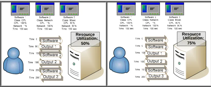
Using DiPred, the scheduler (DiSched) can make better decisions to satisfy the requested duration of the job, where the job should be placed, etc. Since jobs are profiled based on what raw resources they will likely consume and the duration of those resource usage, multiple different jobs could be simultaneously submitted to the same nodes without any significant loss of individual job performance; this would certainly increase resource utilization and as long as the predicted resource usage does not exceed the available resources, the time it takes to complete individual jobs should not be significantly affected. The increase of resource utilization is possible as long as the assumption that several different classes of software can be concurrently executed without significant loss of performance. Figure 2 attempts to explain this very concept of co-scheduling in which 3 different applications belonging to different software classes exhibit different total running time and resource utilization depending on whether the software is run in parallel or in series.
Resource Utilization: 50% Resource Utilization: 75%
Figure 2: Simple example showing that co-scheduling software that has different requirements (in this case CPU and Network resources) could be run in parallel without loss of performance; note that in a serial fashion, it would take 299 seconds to complete all 3 jobs, while if we run the first 2 jobs concurrently, it would
It is expected that Resource Managers could use a combination of resource selection algorithms besides the proposed DiSched component. To ensure that the available resources that the scheduler is aware of is maintained and updated, resource monitoring (i.e. Ganglia, MDS, etc…) will also be necessary. Some current resource managers use resource monitoring to make scheduling decisions, but often only one job is normally submitted to each individual resource. However, combining resource monitoring with predictive scheduling has the potential to not only improve scheduling decisions to yield lower end-to-end job execution times, but to increase resource utilization significantly.
Using DiSched, resource managers / brokers can make more informed decisions regarding resource selection, resource allocation / reservation, load balancing, and satisfying a particular Quality of Service (QoS). There has been much work (Condor, PBS, LSF, MAUI, in clusters and CSF in Grids [20-27]) in the area of resource managers and resource brokers that use the state of current resources to make scheduling decisions. The limitation of this approach is that heuristics must be found that finds relationships between the state of current resources and the application requirements, something that is currently only automatically realized at a basic level. Furthermore, the state of the available resources could both be incomplete and/or stale, and therefore decisions made solely on this state could be suboptimal. Finally, collecting the state of the available resources and always having up-to-date information is not a scalable approach. The overall objective is to develop a scalable resource selection algorithm that utilizes both the state of the current resources and the predictive models that contain dynamic run-time information. The central hypothesis is that current resource allocation algorithms could be improved and as the Grid grows, the problems with the current resource allocation techniques will become even more apparent as the state of the available resources becomes harder to keep up to date. The hypothesis will be tested by the comparison between the proposed resource allocation algorithm and existing approaches; the performance characteristics will be the resource utilization, the flexibility of the approach under varying conditions, and the scalability of the compared approaches. The expected outcome is a scalable resource scheduler that uses both predictive models and available resource information to make better resource scheduling decisions that yield higher resource utilization and that scales along with the growing Grid. My long term career goal is to integrate the proposed resource allocation algorithm into existing resource managers and brokers. Ensuring that the performance of resource managers will be maintained as the size of the systems they coordinate grows will be essential to the scalability of the Grid. The
expected significance consists of the automatic mapping between application requirements and raw resources which would lead to better resource selection algorithms; this essentially would allow higher resource utilization in the Grid, and hence make the Grid more scalable.
The questions that remain unanswered for this section are:
10. Can software performance predictions aid resource scheduling decisions in a consistent and significant manner?
11. Can a broad type of software (that identifies not resource usage, but rather software features, workload, usage patterns, etc) be defined that will most likely benefit from DiSched?
12. Are dynamic run-time performance models more accurate than static generic performance models, especially for certain types of software?
4.0 Preliminary Results
The immediate preliminary results involve validating that the assumptions made in Section 2 are valid:
• Proof that several different classes of software can be concurrently executed without significant loss of performance
• Show that reliable software performance characterization is possible with only a fraction of the entire input space
The long term expected results will be the building of the remaining 3 components (DiProfile, DiPredict, and DiSched) with proof that the proposed approach was able to decreased end-to-end job execution times while increasing resource utilization using predictive scheduling. I expect the entire proposed project to take several years since it involves rather complex issues and it addresses several open problems.
4.1 Testbed
The computer specifications that the experiments were performed on can be found in Table 1. On the other hand, Table 2 shows the actual performance of the 4 main subsystems that we investigated, namely the memory, hard disk, CPU, and network interface. It is interesting to see that both the CPU and the memory subsystems required the use of the CPU extensively, but other subsystems such as the hard disk and network interface card managed to max out their performance with only a fraction of the processor utilization.
Table 1: Computer specifications
Computer Name diablo
Year of Manufacturing 2003 Processor Family AMD K7 Athlon
Processor Clock 2.16 GHz
L1 Cache Data/Code 32K / 32K
L2 Cache 256K
Front Side Bus (FSB) DEC Alpha EV6
FSB Width 64-bit
FSB Clock 332 MHz
FSB Bandwidth 2654 MB/s
Memory Size 512 MB
Memory Bus Type DDR SDRAM
Memory Width 64-bit
Memory Clock 332 MHz
Memory Bandwidth 2654 MB/s Chipset Bus Type Via V-Link
Chipset Bus Width 8-bit
Chipset Clock 531 MHz
Chipset Bandwidth 531 MB/s Network Interface Card NetGear 10/100 PCI NIC Operating System Linux Mandrake 10.1
Table 2: Actual performance of 4 main subsystems: memory, hard disk, CPU, and network interface
4.2 Testing Software
In order to investigate the feasibility of co-scheduling, I developed a “toy” application in C (just a little over 1000 lines of code) that allows the user to specify the amount of resources that the application is to consume. The configuration parameters are:
• t: test length in seconds • tr: number of transactions • cpu: CPU % utilization • mem: memory %s utilization • net: network %s utilization • disk: disk %s utilization
CPU % Performance
mem (MB/s) 100% 423 MB/s
disk (MB/s) 12% 66 MB/s
cpu (MIPS) 100% 886 MIPS
nic (Mb/s) 14% 95 Mb/s
• disk_name: disk file name
• step: granularity between context switches in microseconds • debug: debug messages enabled
The granularity between context switches was implemented using the select() system function allowing a processes to sleep for a predefined amount of time with a granularity of microseconds. I investigated various different values for this step, and found that if the step was too short, the application would spend so much time that it would get really little work done because it would be spending all of its time in the select() system call. I determined that a step size of 10 ms was sufficiently large where the select call did not impose much of a performance penalty on the application, yet it was small enough for the application to be responsive.
Figure 3 below shows a screen shot of the “toy” application with the various parameters and a sample output after running the application for 10 seconds with 75% CPU utilization.
Figure 3: Sample screen shot of the “toy” application using 75% of the CPU
4.3 Co-Scheduling
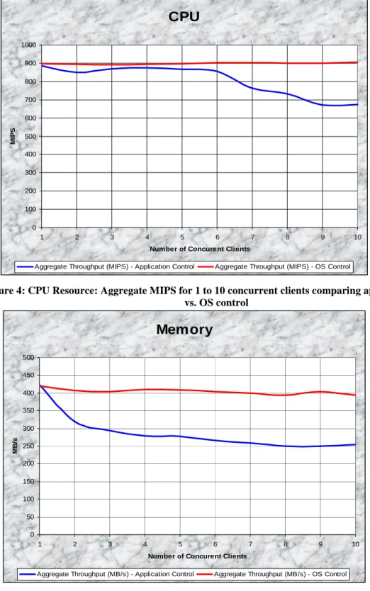
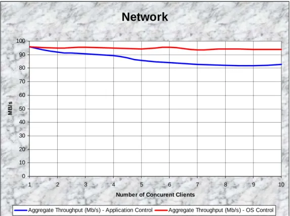
The next few figures depict the performance of the “toy” application and its ability to manage the resource utilization as opposed to the operating systems ability to manage the same set of resources. In all these next experiments, we had two scenarios: 1) 1 to 10 applications that all requested in parallel 100% of a particular resource (red line), and 2) 1 to 10 applications that each requested just partial resource in parallel (blue line), but these partial resources add up to 100% of the resources for each test run. For example, for 10 concurrent clients in Figure 4, the red line represents 10 clients each requesting 100% of the CPU, while the blue line represents 10 clients each requesting 10% of the CPU. We can see that the OS does a very good job of managing the multiple concurrent clients, while my implementation of the “toy” application seems to have a decreasing aggregate performance as the number of clients is increased; this is depicted in Figure 4 - CPU, Figure 5 – MEM, Figure 6 – NET, and Figure 7 - DISK. This can be attributed to the fact that it is unlikely that all various processes managed to enter their sleep states synchronized, and hence there were some overlapping between various processes running
concurrently, and then several processes sleeping concurrently. Unfortunately, this is the reality of co-scheduling multiple processes on the same physical resource, since processes will never be coordinated perfectly in terms of their resource consumption, and hence this phenomenon will be either just as bad if not even worse in the real world.
CPU
0 100 200 300 400 500 600 700 800 900 1000 1 2 3 4 5 6 7 8 9 10Number of Concurent Clients
MI
P
S
Aggregate Throughput (MIPS) - Application Control Aggregate Throughput (MIPS) - OS Control
Figure 4: CPU Resource: Aggregate MIPS for 1 to 10 concurrent clients comparing application control vs. OS control
Memory
0 50 100 150 200 250 300 350 400 450 500 1 2 3 4 5 6 7 8 9 10Number of Concurent Clients
MB
/s
Aggregate Throughput (MB/s) - Application Control Aggregate Throughput (MB/s) - OS Control
Figure 5: Memory Resource: Aggregate MB/s for 1 to 10 concurrent clients comparing application control vs. OS control
Network
0 10 20 30 40 50 60 70 80 90 100 1 2 3 4 5 6 7 8 9 10Number of Concurent Clients
MB
/s
Aggregate Throughput (Mb/s) - Application Control Aggregate Throughput (Mb/s) - OS Control
Figure 6: Network Resource: Aggregate Mb/s for 1 to 10 concurrent clients comparing application control vs. OS control
Disk
0 10 20 30 40 50 60 70 1 2 3 4 5 6 7 8 9 10Number of Concurent Clients
MB
/s
Aggregate Throughput (MB/s) - Application Control Aggregate Throughput (MB/s) - OS Control
Figure 7: Hard Disk Resource: Aggregate MB/s for 1 to 10 concurrent clients comparing application control vs. OS control
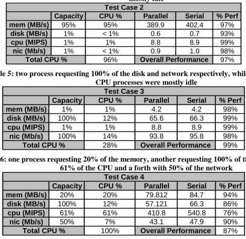
The next few tables show the performance of 4 processes utilizing different subsystems running concurrently on one physical set of resources. Each row represents an individual process, the capacity column indicates the percentage of each respective resource the particular process requested, and the CPU % column represents the actual CPU utilization that particular process utilized. For example, in Table 3, the first process requested 1% of the memory performance, which in turn utilized 1% of the processor as well. The Parallel column represents the performance of the process while it was running in parallel with the other 3 processes. The Serial column represents the performance of the particular process as it solely ran on the physical resource. The % Perf column tries to summarize the performance loss between the parallel performance and the serial performance, with the overall average being found at the bottom right hand corner of each table.
Table 3: one process requesting 95% of the CPU while the memory, disk and network processes were mostly idle
It is interesting that the performance for the first 3 test cases seemed to not be affected significantly due to having several processes running in parallel. Test case 1 has 1 process requesting 95% of the CPU while the rest of the processes sit mostly idle. Test case 2 has 1 process requesting 95% of the memory bandwidth with the rest of the processes sitting relatively idle. Finally, test case 3 has both the network and disk performance maxed out with the memory and CPU relatively idle. At least in these extreme cases, it seems that co-scheduling does not impose a significant performance penalty.
Table 4: one process requesting 95% of the memory while the CPU, disk and network processes were mostly idle
Table 5: two process requesting 100% of the disk and network respectively, while the memory, and CPU processes were mostly idle
Table 6: one process requesting 20% of the memory, another requesting 100% of the disk, another with 61% of the CPU and a forth with 50% of the network
Capacity CPU % Parallel Serial % Perf
mem (MB/s) 20% 20% 79.812 84.7 94%
disk (MB/s) 100% 12% 57.121 66.3 86%
cpu (MIPS) 61% 61% 410.8 540.8 76%
nic (Mb/s) 50% 7% 43.1 47.9 90%
100% 87%
Total CPU % Overall Performance
Test Case 4
Capacity CPU % Parallel Serial % Perf
mem (MB/s) 1% 1% 4.2 4.2 98% disk (MB/s) 100% 12% 65.6 66.3 99% cpu (MIPS) 1% 1% 8.8 8.9 99% nic (Mb/s) 100% 14% 93.8 95.8 98% 28% Overall Performance 99% Test Case 3 Total CPU %
Capacity CPU % Parallel Serial % Perf
mem (MB/s) 95% 95% 389.9 402.4 97% disk (MB/s) 1% < 1% 0.6 0.7 93% cpu (MIPS) 1% 1% 8.8 8.9 99% nic (Mb/s) 1% < 1% 0.9 1.0 98% 96% Overall Performance 97% Total CPU % Test Case 2
Capacity CPU % Parallel Serial % Perf
mem (MB/s) 1% 1% 4.1 4.2 98% disk (MB/s) 1% < 1% 0.6 0.7 94% cpu (MIPS) 95% 95% 825.9 842.3 98% nic (Mb/s) 1% < 1% 0.9 1.0 95% 96% 96% Test Case 1
Test cases 4 and 5 are interesting from the point of view that each process requires a significant amount of resources, and hence the larger contention for the scarce resources (especially CPU), leads the performance loss to be around 15%.
Table 7: one process requesting 37% of the memory, another requesting 100% of the disk, another with 37% of the CPU and a forth with 100% of the network
4.4 Software Characterization
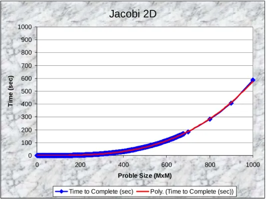
I chose two different problems to investigate, namely the Jacobi 2D problem and the quick sort algorithm. The Jacobi 2D runs in O(n2) and solves a linear system of equations. It is a regular iterative code that continuously updates a 2D matrix within a loop body between some global error-checking stages. This application is an example of a CPU intensive application. The problem size I experimented with were from a 1x1 matrix to a 1000x1000 matrix.
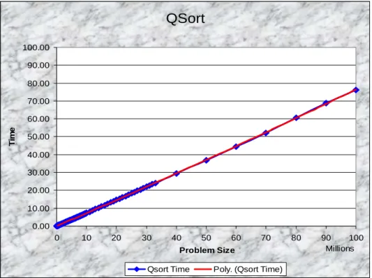
The second problem was the quick sort algorithm that runs in O(n*log(n)). It sorts a list of integers, ranging from a size of 1 to 100,000,000 integers, approximately 1GB of data stored in ASCII text format. Normally, quick sort is a CPU intensive application, however to change the dynamics of the algorithm, I forced the application to read the input data from the hard disk. Although this is a O(n) operation, due the hard disk’s speed being significantly slower than main memory, the time it took to read the data off the disk dominated the running time, and hence the performance of the quick sort algorithm almost appears to be linear; after careful analysis, it can be seen that the graph actually grows faster than linear, but this is only obvious after seeing that a linear approximation does not fit the data perfect.
Figure 8: Jacobi 2D performance running time vs. problem size ranging from 1x1 to 1000x1000 The interesting thing about Figure 8 is the consistency of the time to complete an individual run vs. the problem size. The blue line and markers denote actual performance results, while the red line represents a polynomial
Jacobi 2D
0 100 200 300 400 500 600 700 800 900 1000 0 200 400 600 800 1000 Proble Size (MxM) Ti m e ( sec)Time to Complete (sec) Poly. (Time to Complete (sec))
Capacity CPU % Parallel Serial % Perf
mem (MB/s) 37% 37% 139.3892 156.7 89% disk (MB/s) 100% 12% 57.6732 66.3 87% cpu (MIPS) 37% 37% 250.8 328.1 76% nic (Mb/s) 100% 14% 84.2 95.8 88% 100% 85% Test Case 5
approximation of the empirical results. Note how nicely the last few markers line-up with the polynomial approximation where the problem size is 700, 800, 900, and 1000. As for Figure 9, we see a similar trend where the input size gives us a very consistent time to completion, and the larger sizes of the problem space (50 to 100 million) seem to match perfectly the polynomial approximation.
Figure 9: Quick sort performance running time vs. problem size ranging from 1 to 100 million integers 5.0 Conclusion
This report has covered the following items: • A brief overview of DiPerF
• A literature survey of resource management using predictive scheduling
• Showed that co-scheduling is possible for several different classes of software without significant loss of performance
• Showed that reliable software performance characterization is possible with only a fraction of the entire input space
• A proposal outlining the entire system of components and the related work
• Showed that reliable software performance characterization is possible with only a fraction of the entire input space (at least for 2 specific problems – Jacobi 2D and quick sort)
The proposed work is aimed at developing the following four components with the goals to increasing resource utilization while decreasing end-to-end job execution times using predictive scheduling in the Grid:
1. DiPerF – A Distributed Measurement Framework 2. DiProfile – A Job Profiler for distributed computations
3. DiPredict – Performance Predictions of distributed computations
4. DiSched – Resource scheduling using DiPredict in distributed environments
I believe that the proposed research addresses significant work in the area of performance modeling and resource management. My research work should play a critical role in understanding important problems in the design,
QSort
0.00 10.00 20.00 30.00 40.00 50.00 60.00 70.00 80.00 90.00 100.00 0 10 20 30 40 50 60 70 80 90 100 Millions Problem Size Ti m edevelopment, management and planning of complex and dynamic systems and could enhance the scalability of the Grid as well as improve resources utilization despite the Grid’s growing size.
6.0 References
[1] C. Dumitrescu, I. Raicu, M. Ripeanu, I. Foster. “DiPerF: an automated DIstributed PERformance testing Framework.” IEEE/ACM GRID 2004.
[2] Catalin Dumitrescu, Ian Foster, Ioan Raicu. "A Scalability and Performance Evaluation of a distributed Usage SLA-based Broker in Large Grid Environments", submitted for review to HPDC 2005.
[3] Bill Allcock, John Bresnahan, Raj Kettimuthu, Mike Link, Catalin Dumitrescu, Ioan Raicu, Ian Foster. "Zebra: The Globus Striped GridFTP Framework and Server", submitted for review to HPDC 2005.
[4] C. Lee, R. Wolski, I. Foster, C. Kesselman, J. Stepanek. “A Network Performance Tool for Grid Environments,“ Supercomputing '99, 1999.
[5] A Danalis, C Dovrolis. “ANEMOS, An Autonomous NEtwork MOnitoring System.“ 4th Passive and Active Measurements (PAM) Workshop 2003.
[6] U Hofmann, I Milouchewa1. “Distributed Measurement and Monitoring in IP Networks.“ SCI 2001/ISAS 2001 Orlando 7/2001.
[7] J. L. Hellerstein, M. M. Maccabee, W. Nathaniel Mills III, and J. J. Turek. “ETE, A Customizable Approach to Measuring End-to-End Response Times Their Components in Distributed Systems.” 19th IEEE International Conference on Distributed Computing Systems (ICDCS) 1999.
[8] C. R. Simpson Jr., G. F. Riley: “NETI@home: A Distributed Approach to Collecting End-to-End Network Performance Measurements.” PAM 2004.
[9] R. Wolski, N. Spring, J. Hayes, “The Network Weather Service: A Distributed Resource Performance Forecasting Service for Metacomputing,” Future Generation Computing Systems, 1999.
[10] V. Paxson, J. Mahdavi, A. Adams, and M. Mathis. “An architecture for large-scale internet measurement,” IEEE Communications, August 1998.
[11] R. Wolski, "Dynamically Forecasting Network Performance Using the Network Weather Service", Journal of Cluster Computing, January, 1998.
[12] J. Schopf and F. Berman, “Using Stochastic Information to Predict Application Behavior on Contended Resources," Jrnl. of Foundations of CS, 2001.
[13] Smith, I. Foster, and V. Taylor. “Predicting Application Run Times Using Historical Information”. IPPS/SPDP 1998.
[14] P. Dinda, “A Prediction-based Real-time Scheduling Advisor”, 16th International Parallel and Distributed Processing Symposium (IPDPS 2002).
[15] DA Bacigalupo, SA Jarvis, L He, DP Spooner, DN Dillenberger, GR Nudd, “An investigation into the application of different performance prediction techniques to distributed enterprise applications”, Journal of Supercomputing, 2004.
[16] SA Jarvis, DP Spooner, HN Lim Choi Keung, J Cao, S Saini, GR Nudd. “Performance Prediction and its use in Parallel and Distributed Computing Systems”, IEEE/ACM International Workshop on Performance Modelling, Evaluation and Optimization of Parallel and Distributed Systems, 2003.
[17] F. Vraalsen. "Performance Contracts: Predicting and Monitoring Grid Application Behavior." MS Thesis, Graduate College of UIUC, 2001.
[18] N. N. Tran. “Automatic ARIMA Time Series Modeling and Forecasting for Adaptive Input/Output Prefetching.” PhD thesis, UIUC, 2001.
[19] J. Oly and D. A. Reed, "Markov Model Prediction of I/O Request for Scientific Application," FAST 2002. [20] Irwin D., Chase J., and Grit L., “Balancing Risk and Reward in Market-Based Task Scheduling.” HPDC-13,
[21] Kay, J., and Lauder, P., “A Fair Share Scheduler,” University of Sydney and AT&T Bell Labs, 1988.
[22] "Maui Scheduler, http://www.supercluster.org/maui/." Center for HPC Cluster Resource Management and Scheduling, 2004.
[23] LSF Administrator’s Guide, Version 4.1, Platform Computing Corporation, February 2001.
[24] Condor Project, A Resource Manager for High Throughput Computing, Software Project, The University of Wisconsin, www.cs.wisc.edu/condor.
[25] OpenPBS Project, A Batching Queuing System, Software Project, Altair Grid Technologies, LLC, www.openpbs.org.
[26] I. Foster, C. Kesselman, C. Lee, R. Lindell, K. Nahrstedt, and A. Roy, "A Distributed Resource Management Architecture that Supports Advance Reservations and Co-Allocation," Proc. International Workshop on Quality of Service, 1999.
[27] “Open source metascheduling for Virtual Organizations with the Community Scheduler Framework (CSF)”, Technical White Paper, Platform, 2003.
[28] F. Berman, A. Chien, K. Cooper, J. Dongarra, I. Foster, D. Gannon, L. Johnsson, K. Kennedy, C. Kesselman, J. Mellor-Crummey, D. Reed, L. Torczon, and R. Wolski, "The GrADS Project: Software Support for High-Level Grid Application Development," International Journal of High Performance Computing Applications, vol. 15, pp. 327-344, 2001.
[29] “Connecting Client Objectives with Resource Capabilities: An Essential Component for Grid Service Management Infrastructures,” Asit Dan, Catalin Dumitrescu, and Matei Ripeanu, 2nd International Conference on Service Oriented Computing (ICSOC), November 2004, New York, NY.
[30] George Tsouloupas and Marios D. Dikaiakos. Characterization of Computational Grid Resources Using Low-level Benchmarks. Technical Report TR-2004-5, Dept. of Computer Science, University of Cyprus, December 2004.
[31] George Tsouloupas and Marios D. Dikaiakos. Gridbench: A tool for benchmarking grids. In Proceedings of the 4th International Workshop on Grid Computing (GRID2003), pages 60{67, Phoenix, AZ, November 2003. IEEE.
[32] D. P. Spooner, S. A. Jarvis, J. Cao, S. Saini, and G. R. Nudd. Local Grid Scheduling Techniques using Performance Prediction. IEE Proc. Comp. Digit. Tech., Nice, France, 150(2):87-96, April 2003.
[33] Seung-Hye Jang, Xingfu Wu, Valerie Taylor, Gaurang Mehta, Karan Vahi, Ewa Deelman. Using Performance Prediction to Allocate Grid Resources. GriPhyN Technical Report 2004-25, July 2004.
[34] Eitan Frachtenberg, Dror G. Feitelson, Juan Fernandez-Peinador, and Fabrizio Petrini. Parallel Job Scheduling under DynamicWorkloads. In 9th Workshop on Job Scheduling Strategies for Parallel Processing, June 2003. [35] Eitan Frachtenberg, Dror G. Feitelson, Fabrizio Petrini and Juan Fernandez. Adaptive Parallel Job Scheduling
with Flexible CoScheduling. In IEEE Transactions on Parallel and Distributed Processing. To appear, 2005. [36] Eitan Frachtenberg, Dror G. Feitelson, Fabrizio Petrini, and Juan Fernandez. “Flexible CoScheduling:
Mitigating Load Imbalance and Improving Utilization of Heterogeneous Resources”, IPDPS 2003.
[37] Holly Dail, Henri Casanova, and Fran Berman. A Decoupled Scheduling Approach for Grid Application Development Environments, Proceedings of Supercomputing, November 2002.
[38] Erik Elmroth and Johan Tordsson. A Grid Resource Broker Supporting Advance Reservations and Benchmark-Based Resource Selection, PARA'04 State-of-the-Art in Scientific Computing, June 20-23, 2004. [39] Chuang Liu, Lingyun Yang, Ian Foster, Dave Angulo. Design and Evaluation of a Resource Selection
Framework for Grid Applications, HPDC-11, the Symposium on High Performance Distributed Computing, July 2002, Edinburgh, Scotland.
[40] Valerie Taylor, Xingfu Wu, Rick Stevens. Prophesy: An Infrastructure for Performance Analysis and Modeling of Parallel and Grid Applications, ACM SIGMETRICS Performance Evaluation Review, Volume 30, Issue 4, March 2003.
[41] Ajith Abraham, Rajkumar Buyya* and Baikunth Nath. Nature’s Heuristics for Scheduling Jobs on Computational Grids, the 8th IEEE International Conference on Advanced Computing and Communications (ADCOM 2000), December 14-16, 2000, Cochin, India.
[42] Rich Wolski. Dynamically forecasting network performance using the network weather service. Journal of Cluster computing, 1(1):119–132, 1998.
[43] Ewa Deelman, James Blythe, Yolanda Gil, Carl Kesselman, Gaurang Mehta, Karan Vahi, Kent Blackburn, Albert Lazzarini, Adam Arbree, Richard Cavanaugh and Scott Koranda, Mapping Abstract Complex Workflows onto Grid Environments, Journal of Grid Computing, vol.1, no. 1, pages 25-39, 2003.
[44] Ewa Deelman, James Blythe, Yolanda Gil, Carl Kesselman, Gaurang Mehta, Sonal Patil, Mei-Hui Su, Karan Vahi and Miron Livny, Pegasus : Mapping Scientific Workflows onto the Grid , Across Grids Conference 2004, Nicosia, Cyprus, 2004.
[45] F. Berman, R. Wolski, H. Casanova, et al. Adaptive Computing on the Grid Using AppLeS. IEEE Trans. on Parallel and Distrib. Systems, 14(5), 2003.
[46] C. Liu and I. Foster. A Constraint Language Approach to Grid Resource Selection. Technical Report TR-2003-07, Department of Computer Science, University of Chicago, 2003.