An analytical comparison of nearest neighbor algorithms for load balancing in parallel computers. Creative Commons: Attribution 3.0 Hong Kong License

Title

An analytical comparison of nearest neighbor algorithms for

_{load balancing in parallel computers}

Author(s)

Xu, CZ; Monien, B; Luling, R; Lau, FCM

Citation

The 9th International Parallel Processing Symposium

Proceedings, Santa Barbara, CA, USA, 25-28 April 1995, p.

472-479

Issued Date

1995

URL

http://hdl.handle.net/10722/45548

An analytical comparison

of

nearest neighbor algorithms

for

load balancing in parallel computers

Chengzhong Xu

Department of Eiectrccal and Computer Engg. Wayne State Unavrrsrty, MI 48202

Burkhard Monien, Reinhard Luling

Department of Computer Sccence Unrversrty of Paderborn, Germany

Francis

C.

M.

Lau

Department o j Computer Scrence, The University of Hong h'ong, Hong Kong

Abstract

With nearest nezghbor load balanczng algorzthms, a processor makes balancang decasaons based on ats local anformatron and manages workload magrataons wathan

at5 netghborhood. Thzs paper compares a couple of faarly well-known nearest neayhbor algorithms, the dimen- sion exchange and the diffusion methods and thew varaants an terms of thew performances an both one-port a n d all-port communzcatzon archztdures. It turns out thirt the damensaon ~xchairye method outperforms the daffusion method an the ont -port continunacataon nwdeI, a n d that the strength of the daffuszon method zs an asyn- chronous amplementataons an the all-port communica- taon model The underlying comrnunrcataon networks coiisadered assume the most popular topologzes, the mesh a d the torus and thew b p e r a d cases the hypercubu and

t h e 6-ary n-cube.

1

Introduction

Massively parallel computers have been shown to be very efficient at solving problems that can be parti- tioned into tasks with static compukation and cominu- nication patterns. However, there exist a large class of problems that have unpredictable computational re- quirements and/or irregular commiinication patterns. To solve this kind of problems efficiently in parallel com- put ers, it is necessary to perform load balancing opera- tioiis during run time.

Nearest neighbor load balancing algorithms are a cla.5s of methods in which processors make decisions based on local information in a decentralized manner and manage workload migrations within their neigh- borhood [l, 21. Since they have a less stringent re- quirement on the spread of local workload around the

system, they are scalable t o support massively parallel computers and suitable for retaining the communica- tion locality inherent in the underlying computations. They are also iterative in nature in the sense that suc- cessively imposing local load balancing makes progress t,owards a global balanced state, and hence flexible in controlling the balance quality over the spectrum from the objective of load sharing that assures no idle proces- sors coexist together with busy processors tl, the degree of global balanced state.

Nearest neighbor load balancing algorithms rely on successive approximation to a global uniform distribu- tion, and hence at each operation, need only be con- cerned with the direction of workload migration and the issue of how to apportion excess workloads. There a.re a number of ways for the choice of the direction of workload migration. Among of them, we are inter-. ested in a couple of simple representatives, f h e diflusion

(DF, for short) and the dimension exchange (DE for short) methods. With the diffusion method, a highly or lightly loaded processor balanc.es its workload with all of its nearest neighhors simultaneously in a load balanc- ing operation [3, 41. With the the dimension exchange method, by contrast, a processor in need of load balanc- ing balances its workload successively with its neighbors one a t a time and it,s new workload index will be consid- ered in the the subsequent pairwise balancing [3, 5, 61.

'They are closely related because they lend themselves particularly well to implementation in two basic com- munication architectures, the all-port and the one-port models, respectively. The all-port model allows a pro- cessor t o exchange messages with all its direct neighbors simultaneously in a communication step, while the one- port model restricts a processor t80 exchange messages with at most one direct neighbor a t a time. Both of these two models are valid in real parallel computers

and were assumed in many recent, researches on com- munication algorithms ([7], for example).

The all-port and one-port models favor the diffusion and the dimension exchange methods, respectively. In a system t h a t supports d-port concurrent communica- tions, a load balancing operation using the diffusion method can be completed in one communication step while that using the dimension exchange method would take d steps. I t appears that the diffusion method has an advantage over the dimension method as far as ex- ploiting the communication bandwidth is concerned. A

natural but interesting question is whether the advan- tage translates into real performance benefits in load balancing or not. The performance of a load balanc- ing algorithm is determined by t8wo measures. One is elgiciency which is reflected by the number of communi- cation steps required by the algorithm t o drive an initial workload distrisution into a uniform distribution. This measure alone is sufficient for those kinds of problems that need global balancing a t run time. However, for the other kinds of applications that need t o achieve load sharing rather than global balancing, we need another measure, the balance qualaty, t o reflect the ability of the algorithm in bounding the variance of processors' workloads after performing one or more load balancing operations. The objective of this study is t o answer the question concerning tlie performance of thP diffu- sion and the dimension exchange methods in different communication models.

In this paper, we make a comprehensive compari- son between the diffusion and the dimension exchange methods with respect to their efficiencies and balanc- ing qualities when they are implemented in both one- port and all-port communication models, using syn- chronous/asynchronous invocation policies, and with static/dynamic random workload behaviors The com- munication networks to be considered include the struc- tures of n-D torus and mesh, and their special cases: the ring, the chain, the hypercube and the IC-ary n-cube. We limit our scope to these structures because they are the most popular choices of topologies in commercial parallel computers

[SI.

Both the dimension exchange and the diffusion meth- ods are parameterized algorithms, and their perfor- mance is largely influenced by the choice of the pa- rameter values. We focus on two choices of the pa- rameter value in each method: the iwerage DE (ADE),

the optimally-tuned DE (ODE), the local average DF

(ADF), and the optimally-tuned DF (ODF). The opti- mality here is in terms of the efficiency in static syn- chronous implementations among various choices of the DE and the DF parameters The average versions (ADE

and ADF) are the most original versions and are still being employed in real applications today; we there- fore include them in our comparison. Our main results are that the dimension exchange method outperforms the diffusion method in the one-port communication model; in particular, the ODE algorithm is found t o be best suited for synchronous implementation in the static situation; and that the dimension exchange method is most superior in synchronous load balancing even un- der the all-port communication model; the strength of the diffusion method is in asynchronous implementation under the all-port communication model; the ODF al- gorithm performs best in high dimensional networks in this case.

The rest of paper is organized as follows. Section 2 provides a framework of load balancing for our com- parison of the various algorithms. Section 3 specifies load balancing algorithms in a unified forni. Section

4

compares load balancing algorithms when lhey are im- plemented in asynchronous and synchronous invocation policies. Section 5 reports the results from simulations that further assess the load balancing algorithms. We conclude in Section 6 with a summary of comparative results for the DE and the DF methods.

2

A

generic model of load balancing

The parallel computer we consider is composed of a fi- nite set of homogeneous processors, which are intercon- nected by a direct communication network Processors communicate through passing messages. The communi- cation channels are assumed t o be full duplex so that a pair of directly connected (nearest neighbor ) processors can send/receive messages simultaneously t, )/from each other. In addition, we assume the sending and the re- ceiving operation of a message in two ends of a channel take place instantaneously. We represent such a system by a simple connected graph G

=

( V , E ) , where V is a set of processors labeled 1 through N , and E' V x V is a set of edges. Every edge ( i , j ) E E corresponds to the communication channel between processors i and j. Let

d(i) denote the set of nearest neighbors of processor i, d(i)

=

Id(;)/

be the degree of processor i, and d(G) be the maximum of d ( i ) for 1

5

i

5

N .

The underlying parallel computation is assumed t o comprise a large number of independent processes, which are the basic units of workload. The total num- ber of processes are assumed to be large enough so that the workload of a processor is infinitely ditisible. Pro- cesses may be dynamically generated or consumed as

the computation proceeds, and may also l)e migrated

across processors for the purpose of balancing. Cor- respondingly, we distinguish between two fundamental operations in a processor by their purposes: the compu- tational operation and the balancing operation. An any time, a processor is performing a computational opera- tion and/or balancing operation. Notice that during the execution of a balancing operation, the underlying com- putation can be suspended or performed concurrently. The concurrent execution of these two operations is pos- sible when processors are capable of multiprogramming or the balancing operation is done in the background by cheap coprocessors. Since the workload of processors is either fixed or varying with time in the load balancing process, we refer t o these two execution cases as SlQtZC arid dynamzc situations, respectively.

Let

t

be an integer time variable, which is propor- tional to global real time. We quantify the workload of processor i a t time

t

by w: in terms of the number of residing processes. Let

z ( t )

denote the set of proces- sors that are performing balancing operations a t time

t . Then, the change of workload of a processor a t time

t in the dynamic situation is modeled by the equation

where

4fti

denotes i,he aniounts of workload generated or finished from time t to t

+

1, aiid

ft(.)

represents a load balancing operator.

aft'

= 0 in the static situa- tion.

This model is generic because the. balancing operator

f l ( . ) and the set of processors in load balancing at any

time

t , z ( t ) ,

are left undefined. The operator

ft(.)

can bc any nearest neighbor load balancing algorithms in- cluding the diffusion and the dimension exchange meth- ods, which will be sperified in t h c next section. The set I ( t ) is determined by invocation policies of load balancing. They are orthogonal tc) load balancing al- gorithms in that any invocation policy can he iniple- mented in combination with any b a d balancing algo- rit hm. Since a load balancing operat,ion incurs nonneg- ligible overheads, different applications require tliffcbrent invocation policies for better tradeoff between their ben- efits and extra overheads In parallel computations us- ing domain decomposition techniques for example, the computational requirement. associated with each por- tion of a problem domain may didnge as the coIripu- tation proceeds. To reduce the p i a l t y of load inibal- arices, an effective way is to periodically redecoinpose the problem domain with the aini of achieving a. global uniform distribution arross processors. To this end, all processors are required to perform load balaiicing oyterations synchronously for a shtrrt period. That is,

I(t)

= {

1 , 2 ,

,

. . .

,

N } for t

3

t o , where to is the instant when the whole system state satisfies certain conditions

as those set in [9]. By contrast, the parallel execution of dynamic tree-structured computations usually requires only local balancing which assures no idle processors exist while there are other busy processors. Thus, each processor is allowed t o invoke a load balancing opera- tion a t any time in an asynchronous manner according to its own local workload distribution. A simple pol- icy is that once a processor's workload drops below a preset threshold, wunde+,ad, a load balancing operation is then activated. That, is, T(t) = {ilwj

<

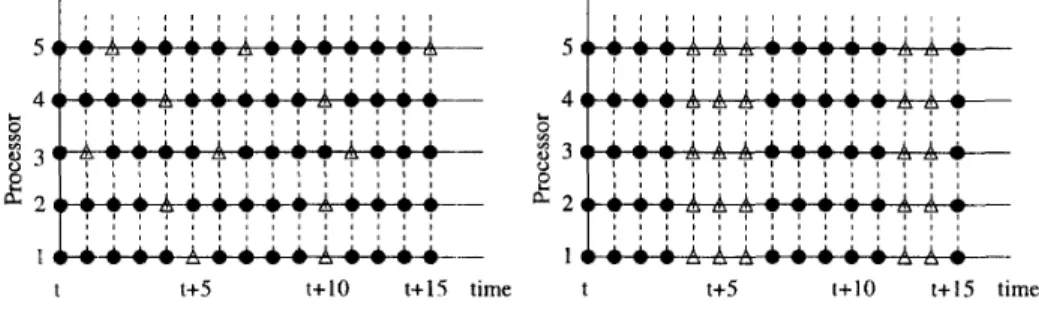
Wunderload}.

More sophisticated invocation policies were discussed in [lo, 21. Figure 1 presents an illustration of these two implementation models in a system of five processors. The dots and the triangles represent the computation operation and balancing operation, respectively.

3 The dimension exchange versus the

diffusion methods

This section briefly describe of the dimension ex- change and the diffusion methods. Both of them are parameterized algorithms. We present several instances of these two methods based on different choices of values for their parameters.

3.1

The dimension exchange method

With the dimension exchange method, any processor which invokes a load balancing operation balances its workload with its neighbors successively. I'or a proces- sor i, it works in the following way that

where j , E d(i), and 0

<

X

<

1, called the dimension exchange parameter, is preset t o determine the fraction of excess workload to be migrated between a. pair of pro- cessors. The formula tells that a balancing operation in the dimension exchange method comprises d ( i ) pairwise balancing steps for processor i . At each step, processor i balances its workload with one of its neighbors, and uses the new result for the subsequent balancing. It is because of the sequential nature in the sequence of bal- ancing steps, a load balancing operation requires d ( i )

communication steps in both the all-port and the one- port communication models.

The efficiency of the DE method is determined by the dimension exchange parameter. A DE operation with different choices of the parameter will reduce the

5 5 4 4 c L si 2 3 3 I --- 1 % 8 3 E 2 a 2 I , , , , , , , , , t t+5 t+10 t+lS time t t+5 t+10 t+15 time

(a) Asynchronous implementation (b) Synchronous implementation Figure 1: An illustration of generic models of load balancing

imbalance factor of a system state t y different factors. In t,he following, we present two choices of the parameter which have been suggested as rat,ional choices in the litcrature

I Average damenbzon erthange ( A D E ) equally splits the total workload of a pair 01 processors by the choice X

= 1 / 2 It is

a straightforward choice for local balancing at each pairwise operation, and has been favored in hypercuhe netucrrks [3]

2 Optamally-funned dinif nsaon exchange (ODE) is a new variant of the DE method, which takes certain specific parameter values that have the effect of maximizing efficiency i n global balancing [ll]. The optimal parameter depends on the topology and the size of underlying coinmunic ation network Let k

=

max{k,, 1

5

i

5

n } in the

k~

x x C, mesh and torus 'Then, their optimal parameter values were shown, in [ l l ] , as

0 X

=

1/( 1

+

sin(ir/k)) in the mesh, 0 X = I / ( 1

+

h i n / h / k ) ) in the toriis 3.2

The diffusion method

With the diffusion mrbthod, any processor which in- vokes a load balancing operation compares its workload with those of its nearest neighbors, and then gives away o r takes in certain airioiint of workload with respect, to rac h nearest neighbor. The diffusion operator in a pro- cessor i can be written in the form that

workload Iwi - wj

I

t o processor j if wi

>

wj

,

or fetches some workload from processor j otherwise. Clearly, a load balancing operation with the I > F method requires only one communication step in t,he all-port, communi- cation model, but d ( i ) steps in the one-port. communi- cation model.

As in the DE method, the efficiency of the D F method is determined by the diffusion parameter. Following are two common choices of the parameter.

1 . Local average dzflusion (ADF) takes an average of workload of neighboring processors by setting a" z J

-

- [12, 131. The torus is regular in t,hat

processors have the same degree. The mesh is ap- proximately regular when i t is in large size. For simpIicit.y, we nse a single value cr =

&

to cover all communication channels in the mesh and the torus.

2 . Opiimally-tuned dzflusion (ODF) is ii new vari-

ant of the DF method, which takes certain spe- cific parameter values for maximizing efficiency in global balancing [3]. As in the DE method, the optimal diffusion parameter depends on the topol- ogy and the size of underlying networks. Let

k

=

max{ IC1 , k 2 , .

.

. ,

k,}

in the IC1 x kz x I

.

kn mesh and torus. Then, their optimal choices were shown, in [3, 141, as

0 LY = 1/2n in the mesh,

0 CY = l / ( 2 n

+

1

-

c o s ( 2 7 r / k ) ) in thc torus, 0 a

=

l / ( n

+

1) in the n-D hypercube.

where 0

<

cyzJ

<

1 , called the diffusion parameter, is

prt,defined t o dictate the portion to be migrated be- t,wchen any two processors. I'rocessor i apportions excess

Assume t = 0 when processors invoke a synchronous or asynchronous load balancing procedure. We are con- cerned with subsequent workload distributions resulting

from different load balancing algorithms. Denote the overall workload distribution a t certain time t by a vec- tor W t

=

(tu;, wi,. .,U$,,). Denote its corresponding uniform distribution by a vector

p t

=

(E',

z', .

' , G'),

where E'

=

CL,

wi/IV. We define a concept of system ambulance factor, denoted by u t , as the deviation of W t from

W'.

That is, vt

=

~ [ W t - ~ t ~ ~ '

=

E?

a = ]

( ~ 1 U f - - ~

w

1

.

The system imbalance factor reflects the variance of pro- cessors' workloads at a given point in time.

With the system imbalance factor u t l we define the efficiency of a load balancing algorithm, denoted by T ,

a5the number of load balancing steps required to re-

duce the imbalance factor of the initial state t o a toler- able level in the static situation; and define the balance quality as the bound for imbalancr factors which is t o

br guaranteed by the load balancing procedure III the

d j namic situation. Load balancing algorithms will be compared with each other in terms of these two rnea- stires under the following assumptions. Throughout the section,

E[.]

denotes the expected value of a random variable.

Assumption 4.1 A t initial time, processors' work-

loads wp, 1

5

i

5

N , are N andepen,dent and identically distributed 6.i.d.) random variables with expectation ,UO

and variance U:. A t any t i m e t ,

t

2

0 , processors' work-

load generation/'con~surription rataos

&,

1

5

i

<

N , are

zero in the static situation or i.i.d. random variables wrth expectation ,U and variance U' zn the dynamic sit-

u tit ion.

4.1 Asynchronous implementations

In an asynchronous implementation of load balanc- ing, processors perform load balancing operations dis- cretely based on their own local workload distributions and invocation policies. Since load balancing algorithms can be treated as orthogonal t o their invocation policies, w e consider the load balancing operations of processors in one time step so as to isolate their effects on the sjstem imbalance factor from the effects of invocation policies. We focus OIL the static situation of load balanc-

ing in which the underlying computation in a processor

i:, suspended while the processor is performing load bal-

aiicing operations. The dynamic situation makes only a few differences to the analysis of the effects of load halancing.

Let uo be the original system imbalance factor when

t

=

0, and U' be the system imbalance factor when

t = 1. Our comparison will be made between

vider u i d f , and uidj which are resulting from various load balancing Operations

Theorem 4.1 Suppose processors are running an asynchronous load balancing process under Assump- tion 4.1. Then, E[uAde]

5

E[ufif] in the one-port com- munication model, while E[uLtf]

5

E[uide] En the all-port communzcation model. Moreover, E [ u i d f ]

5

E[uidf] in the chain and the rang networks but E[u,',,]

5

E[v&]

in two- or higher- dimensional meshes and tori. I n ad- dition, E[uide]

<

E[u,lde] 2n the all-port cornmunicataon model.

The comparison is based on a lemma concerning the sample variance of a combination of random variables in a sample set. We present it without proof. It can be easily shown using fundamental statistical theories. Lemma 4.1 Suppose that (1 ( 2 , . .

. ,

( N are N i.i.d random variables with vanance U', and

<

=

CE,(i.

Then,

1 . for any k , 15 k

<

N ,

where 0

<

a;

<

1 satisfying

variance is minimized at ai = l / k f o r a given

k.

ai = 1 ; and the

2. f o r any kl and k2 and 1

<

k1

5

k2

5

N ,

where 0

<

ai

<

1 satisfying bi

<

1 satisfying

a; = 1 and 0

<

b j

=

1 .

Proof sketch of Theorem 4.1 At certain time in an

asynchronous load balancing process, there might be more than one processor which are invoking load bal- ajcing within their neighborhoods simultaneously. Let d ( i )

=

{i}

U d(i) denote the balancing domain of an invoker processor i . The balancing domains of concur- rent invokers may be overlapping or separated with each other. As a whole, those processors which are running load balancing processes are partitioned into a number of separated spheres, some of which are singular balanc- ing domains and some of which are unions of overlap- ping domains. Processors in different spheres perform load balancing operations independently, while proces- sors in the same sphere perform load balancing in a synchronous manner.

Suppose initially there are m independent balanc- ing spheres in the system, denoted by

B1

,

B2,

. . . ,

Bm.

Then, by the definition of the system imbalance factor

v , we have

N N

The last term is a constant for a given number of pro- wssors in load balancing and independent of the topo- logical relationships among the processors in load bal- ancing. The first term is due to load balancing oper- ations in all separated balancing spheres. It is a sim- ple arithmetic sum of imbalance factors of each sphere,

~ ~ : r E B J E(lwf

--

GII')). As a whole, E[v'] implies that the expected value of the system imbalance factor is influenced independently by load balancing operations within different balancing spheres Therefore, it suf- fices t o compare the effects of load balancing algorithms within different spheres using Lemma 4.1 Owing to the limitation of space thc remainder of the proof is omit- ted here.

This theorern says that the dimmsion exchange and the diffusion methods are suitable for the one-port and the all-port communication models, respectively. More specifically, it reveals that the ODF algorithm outper- forms the ADE' algorithm in higher dimensional meshes arid tori although the ODF was originally proposed for iise in synchronous global balancing

4.2 Synchronous implementations

In a synchronous implementation of load balancing, processors perform load halancing operations concur- rently and continuously for a timc: period in order to achieve a global balanced state in the state situation or t(J keep the varying system imbalance factor bounded in the dynamic situation. From Eq. (2) and (3), it is kiiown that both t h e balancing operators,

ti(.),

of the DE and the DF methods are linear iterative operators. Hence, the synchronous implementation of Eq (1) can

t l t b modeled by the equation

Wt+' = FWt

+

@*, ₍₆₎

where F is either a IIE or a DF matrix defined by Eq. (2) or (3), respectively The features of synchronous imple- mentations of the DE or DF methods are therefore fully captured by the iterative process governed by F.

In the static situation, cpt = 0. According to funda- mental iterative theoritas, we then have

?'= 0 ( 1 / I n y ( F ) ) , (7)

where y ( F ) is the subdominant eigenvalue of F in mod- ulus. The closed expressions of y(F) are readily avail- able in [12, 111 when the DE and the DF methods are applied in the mesh and the torus networks. Substi- tuting them in Eq.(7), we obtain the efficiencies of the DE and the DF methods in both one-port and all-port communication models, as presented in Table 1.

The entries of the table show that both the ADE

and the ODE algorithms converge asymptotically faster than the diffusion method in the one-port communi- cation model; and that in the all-port communication model, the ODE algorithm converges also faster than other three algorithms by a factor of

k.

In the dynamic situation, Eq.(7) leads to that E [ d ] = E(IIWt

-

Wf112)

-

-

E ( ( p W t - 1

-

V y )

+

E ( p t

-

(a"12) = E ( ( ( F f + l W "

-

t + CE(((p@+1-i

-

$ + I - i = O

From Lemma 4.1, we then obtain that with the DE method in the one-port model,

where b = ( l - X ) 2 + X 2 a n d s = 1 + b + b 2 + . . . + b d - l ; and with the DF method in the all-port model,

1

--

at+l I - U

E [ 4 ] = (U"".;

+

-

a 2 ) N

-

( t

+

l ) a 2

-

U ; ,

where U = (1 - da)'

+

do2. Easily, we come to the following theorem.

Theorem 4.2 Suppose processors are running syn-

chronous DE and DF load balancing processes under Assumption 4.1. Then, E[.:&]

5

E [ Y : ~ ~ ] , E [ v : ~ ~ ]

5

E[v:dj], and E[&]

5

E[&j] in both one-port and ail- port communication models.

5

Experimental results

In the preceding section, we explored a number of relationships between the dimension exchange and the diffusion methods with respect to their efficiencies and balancing qualities. In order to obtain an idea of the magnitude of their differencies, we conducted a statis- tical simulation of these load balancing algorithms on various topologies and sizes of communication networks and on synthetic workload distributions. The experi- mental results also serve to verify the theoretical results.

Table 1: Efficiencies of load balancing algorithms in the mesh and torus networks, where k is the maximum number of nodes over all dimensions in an n-D network and

*

- port means the all-port communication model

ADE ODE ADF ODF

torus mesh

I n the simulation, the initial workload distribution

W

is assumed t o be a random vector, each element w of which is drawn independently from an idmtical uni- form distribution in [0, l O O O ] Each d at a point obtained in the experiment is the average of 20 runs, using dilfer-

mi random initial workload distributions and different workload generation ratios We also assume t h r un- derlying system is in all port communication model so that a DE balancing operation takes the time of 2 n DF opt rations in the n-1) niesh and t h e n - D torus. A DF optaration is taken as a b m i c time step in a load balanc ing process.

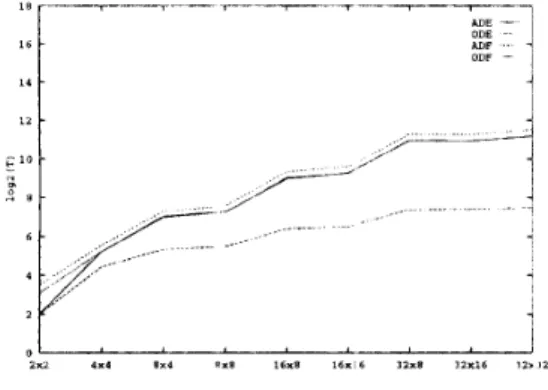
‘The first experiment IS a simulittton of ss nchronous load balancing in the static behailor of workloads. In thc simulation, we measure the riuntber of cornrniini- cation steps, denoted by Z’, necess,try for arriving a t a tlobal balanced state We define the global balance s t d e as the state in which system imbalance factor is less than or equal to one Figure 2 plots the experiinen- tal results from different load balancing algorithms in thfl 2-D mesh of’ various sims from 2 Y 2 to 32 x 32

I

1--port8 *-port 1-port *-port 1-port *-port 1-port *-port

O ( n k 2 ) O ( n k 2 ) O(nk) O(nk) O(n2k2) O ( n k z ) 0 ( n 2 k 2 ) O ( n k 2 ) O ( n k 2 ) O ( n k 2 ) O(nk) O(nk) O(n2k2) O(nk2) O ( n 2 k 2 ) O(nk2)

change method out performs the diffusion ntethod even in the all-port communication model. In ptuticular, it is seen that the ODE algorithm accelerates the DE load balancing process significantly. In Figure 2, we also see that the number of communicatioii steps

r

in a 2-D niesh is dependent only on the size of it,s 1ii.rge dimen- sion and insensitive to the size of its small dimension. This observation was proved to be true in both the mesh and the torus in [l 11.

The second experiment is a simulation of asyn- chronous load balancing in the dynamic situation of ran- dom workload gent:rations/consumptions. In the sim- ulation, we assume the expected workload generation ratio of a processor at each time step is 100 with the variance of 30 and the consumption ratio is a constant

LOO. In the simulat,ion of asynchronous load balancing,

we use a simple invocation policy that once a processor’s workload drops or rises beyond a pair of preset bounds, ‘LOO and 800, the processor then activates a load balanc- ing operation. Figure 3 plot,s the system iml)alance fac- tors resulting from different load balancing algorithms in a mesh of size 16 x 16.

0

0 0 100 I50

Figure 2: The number of necessary communication steps during a statically synchronous load balancing process in the 2-D mesh of various sizes from 2 x 2 to 32 x 32

This figure clearly indicates that t.he dimension ex-

0

Figure 3 : Change of the system imbalance factor in the first 200 steps of a dynamically asynchronous load balancing process in the rnesh of size 16 x 16

duces the initial system imbalance factor more rapidly than the diffusion method and keeps it bounded in a much lower level. It can also be observed that both the ODE and the ODF algorithms, the optimally tuned al- gorithms for global synchronous load balancing, do not gain significant benefits in asynchronous implementa- tions.

6

Conclusions

In this paper, we made a comparison between two classes of nearest neighbor load balancing algorithms, tht. dimension exchange (DE) and the diffusion (DF) mcthods, with respect to their efficiency in driving any initial workload distribution t o a uniform distri- bill ion and their ability in controlling the growth of variance among processors' workloads. We focused on thvir four instances -the ADE, the ODE. the ADF ant1 the ODF--which are the most common versions in practice. The comparison was made comprehensively in both one- port and all- 11 or t com mimic a t ion models

with consideration of various implementation strate- gieli: synchronous/asynchrorious invocation policies and stnticldynamic random workload behaviors.

We showed that the DE method outperforms the DF method in rhe one-port, communication model. In particular, the ODE algorithm is best suited for syn- chronous implementation in the static situation. We also revealed of the superiority of the DE method in synchronous load balancing even in the all-port conimu- nication model. The strength of the diffusion method is i n asynchronous implementation in the all-port com- inunication model. The OIIF algorithm performs hest in high dimensional networks in that case.

'I'he comparative study not only provides an insight into nearest neighbor load balancing algorithms, but also offers practical guidelines t o system developers in designing load balancing a1 chitectures for various par- allc 1 computational paradigms.

References

[ k J V. Kumar, A. Y. Grama, and N R. Vempaty. Scal-

able load balancing techniques for parallel comput- ers. Journal of Parallel and Dastrzbuted Computmg, 22(1):60-79, July 1994.

[2\ M . Willebeek-LeMair and A. P. Reeves. Strategies for dynamic load balancing on highly parallel com- puters. IEEE Transactzons on Parallel and Das-

trzbuted Systems, 4(9):!279-993, September 1993.

[3] G. Cybenko. Load balancing for distributed mem- ory multiprocessors. Journal of Parallel and

Dis-

tributed Computing, 7:279-301, 1989.

[4] D. P. Bertsekas and J . N . Tsitsiklis. Parallel and distributed computation: Numerical methods, Prentice-Hall Inc., 1989.

[5] B. Ghosh and S. Muthukrishnan. Dynamic load balancing in distributed networks by random matchings. In Proceedings of 6th ACM Symposium on Parallel Algorithms and Architectures, 1994. [6] C.-Z. Xu and F.C.M. Lau. Analysis of the gen-

eralized dimension exchange method for dynamic load balancing. Journal of Parallel and Distributed Computing, 16(4):385-393, December 1992. [7] S . L. Johnsson and C.-T. Ho. Spanning graphs

for optimum broadcasting and personalized com- munication in hypercubes. IEEE Transactions on Comput ers, 38( 9) : 1249- 1268, Septembt :r 1989. [8] L. M. Ni and P. K . McKinley. A survey of worm-

hole routing techniques in direct networks. IEEE

Computer, 26:62-76, February 1993.

[9] D. M. Nicol and P. F. Reynolds. Optimal dynamic remapping of data parallel computation. IEEE

Transactions o n Computers, 39(2):206-- 219, Febru- ary 1990.

[lo] R. Liiling and B. Monien. A dynamic distributed load balancing algorithm with provable good per- formance. In Proceedings of 5th A C M Symposium on Parallel Algorithms and Architectures, pages 164-172, 1993.

[ l l ] C.-Z. Xu and F M . Lau. The generalized dimen- sion exchange method for load balancing in %-ary n-cubes and variants. Journal of Pa.rallel and Dis- tributed Computing, 21( 1):72-85, January 1995. [I21 J . B. Boillat. Load balancing and poisscm equation

in a graph. Concurrency: Practice and Experience, 2(4):289--313, December 1990.

[13] X . 3 . Qian and Q. Yang. Load balancing on gen- eralized hypercube and mesh multiprocessors with lal. In Proceedings of 11th International Conference on Distribuied Comp,uting Systems, pages 402-409, 1991.

[14] C.-Z. Xu and F.C.M. Lau. Optimal parameters for load balancing with the diffusion method in mesh networks. Parallel Processing Letlers, 4(2):139- 147, June 1994.