IOWA STATE UNIVERSITY
Department of Economics
Working Papers Series
Ames, Iowa 50011
Iowa State University does not discriminate on the basis of race, color, age, religion, national origin, sexual orientation, gender identity, sex, marital status, disability, or status as a U.S. veteran. Inquiries can be directed to the Director of Equal Opportunity and Diversity, 3680 Beardshear Hall, (515) 294-7612.
Termination of Dynamic Contracts in an Equilibrium Labor Market Model (2008 update)
Cheng Wang
July 2005
Termination of Dynamic Contracts
in an Equilibrium Labor Market Model
Cheng Wang
∗Earlier versions: 2004, 2005, 2006, 2007
This version: July 2008
Abstract
In an equilibrium model of the labor market, workers and firms enter into dynamic contracts that can potentially last forever, but are subject to optimal terminations. Upon termination, the firm hires a new worker, and the worker who is terminated receives a termination contract from the firm and is then free to go back to the labor market to seek new employment opportunities and enter into new dynamic contracts. The model permits only two types of equilibrium terminations that resemble, respectively, the two kinds of labor market separa-tions that are typically observed in practice: involuntary layoffs and voluntary retirements. The model allows for the simultaneous determination of a large set of important labor market variables including equilibrium unemployment and labor force participation. An algorithm is formulated for computing the model’s equilibria. I then simulate the model to show quantitatively that the model is consistent with a set of important stylized facts of the labor market. Keywords: dynamic contract, termination, labor market equilibrium
JEL Codes: E2, J41, J63
∗Department of Economics, Iowa State University, Ames, IA 50011, U.S.A. Email:
1
Introduction
In an equilibrium model of the labor market, jobs are dynamic contracts, job sep-arations are terminations of dynamic contracts. Matched workers and firms enter into dynamic contracts that can potentially last forever, but are subject to optimal terminations. Moral hazard is the information friction, that contracts are dynamic and terminations are part of the optimal contract are both motivated by incentive considerations. Upon termination, the firm hires a new worker, the terminated worker receives a termination compensation contract from the firm, and is then free to go back to the labor market to seek new matches and enter into a new contract, or to stay temporarily or permanently out of the labor market.
The model thus allows for the simultaneous determination of the size and com-position of the economy’s equilibrium employment, unemployment, and retirement. Most existing equilibrium models of the labor market focus on the interaction between employment and unemployment, without modelling explicitly the state of not-in-the-labor-force and hence the size of the labor market. 1 Also endogenously determined in the model is the economy’s equilibrium labor turnover (flows between employment and unemployment, and the flow into retirement), as well as a set of other impor-tant labor market variables, including the dynamics and distribution of wages and expected utilities of employed workers, the distribution retired workers, the starting expected utility of newly hired workers, and the equilibrium expected utility of the new labor market entrants.
Despite potentially complicated dynamics that may arise in the model environ-ment, the equilibrium of the economy has a simple structure regarding termination. Specifically, the model permits only two types of equilibrium terminations that re-semble, respectively, the two kinds of labor market separations that are typically observed in practice: involuntary layoffs and voluntary retirements. When an invol-untary layoff occurs, the firm promises no future payments to the worker, and the expected utility of the worker is strictly lower than that of the new worker the firm hires to replace him. When a voluntary retirement occurs, the worker leaves the firm with a termination compensation that is equal to a sequence of constant payments, and he never goes back to the labor market to seek new employment again.
Unemployment is involuntary in my model, as in the models of efficiency wages ( e.g., Shapiro and Stiglitz, 1984; MacLeod and Malcomson, 1989). Compared to the
1For example, Mortensen and Pissarides (1997), Shimer (2005), Moscarini (2005), Nagypal (2005).
Sun-Bin Kim (2001) and Moscarini (2003) are exceptions. In both papers though, an additional source of worker heterogeneity is introduced into the Mortensen-Pissarises framework in order to generate flows into retirement. In Moscarini (2003) for example, the productivity of a match depends on a match specific variable, as well as a non-match-specific variable that captures the ability of the worker. The values of both variables are learned during a match, workers whose non-match-specific variable are learned to be sufficiently low choose to withdraw from the labor market. In my model, the simultaneous modelling of the three states of the labor market is based on a single information friction.
efficiency wage models, my model offers at least three advantages. First, efficiency wage models are often criticized because the employment contracts in these models are not fully optimal (Carmichael, 1985). In Shapiro and Stiglitz, for example, because wages are constant, termination (lay-off) is the only incentive device that firms have available to prevent workers from shirking. 2 In my model, workers and firms enter into explicit and fully optimal dynamic contracts where wages vary optimally with the worker’s performance history. Second, in the existing models of efficiency wages, in equilibriumnoworkers are actually fired. The contract makes effort-making incen-tive compatible so no one shirks, and the unemployed are a rotating pool of workers who quit for reasons that are exogenous to the model. In the model here, workers are actually fired involuntarily from their jobs: firing is part of the model’s equilib-rium path. Third, my model permits simultaneously involuntary unemployment and voluntary retirement as its equilibrium outcome.
The economic logic for the equilibrium voluntary retirement in my model is in-tuitive. Because of the worker’s decreasing marginal utility of consumption, the cost of compensating the worker for a given amount of effort is higher as the worker’s expected utility increases. On the other hand, the way that incentives are provided optimally in this environment requires that each time the worker produces a high out-put, he is rewarded with a higher expected utility. Imagine now the worker produces a sequence of high outputs to make his expected utility sufficiently high. Then it will become too expensive for the firm to compensate for the worker’s efforts, and the firm will then find it efficient to replace the worker with an unemployed worker whose efforts are less expensive. The worker leaves the firm voluntarily, for his expected utility is not reduced upon termination. The worker will not go back to the labor market after termination, because other firms also would find him too expensive to employ.
In the model, retirement is optimal and determined by the worker’s history of performance and the cost of the new worker that the firm could hire to replace him. Retirement is an incentive and compensation consideration. It occurs as a conse-quence of firms efficiently motivating and compensating their workers. Retirement is not a life-cycle consideration, as the workers are “perpetually” young (they die with a constant probability) in my model. Retirement does not depend on the worker’s tenure per se, although it does depend indirectly on the worker’s tenure because it takes time before the worker’s expected utility becomes sufficiently high to justify retirement. There is not a unique retirement date in my model. There is a set of performance histories that can all lead to voluntary retirement. This property of my model differentiates it from Lazear’s (1979) theory of mandatory retirement, which is based mainly on job tenure. In Lazear, it is imposed that there is a deterministic date
T after which the worker’s reservation wage exceeds his value of marginal product,
2MacLeod and Malcomson (1989) avoids this critique by modelling employment as a repeated
and T is the retirement date. 3
This paper offers an alternative to the existing theories of equilibrium worker turnover (job separation). Existing models of equilibrium turnover are built around a key variable: the productivity or quality of the job match. In the existing models, it is the evolution of the true or perceived quality of the current job match that provides an engine for job separation. In Jovanovic (1979) and Moscarini (2005), turnover occurs after the firm and the worker have learned enough about the true quality of the current job match. In Hopenhayn and Rogerson (1993) and Mortensen and Pissarides (1994), separation occurs after a stochastic but exogenous process takes the productivity of the current match to a sufficiently low level. In the models of on-the-job-search, matches dissolve after the arrival of new matches with a higher level of productivity.4 I take a dynamic contract point of view to modelling equilibrium worker turnover in this paper. Worker turnover is motivated by the provision of dynamic incentives and risk sharing. Workers and firms are homogeneous in my model, and all matches are identical: they operate the same production function in all periods. Termination occurs not because the technology of the current match has evolved to be sufficiently poor as in Mortensen and Pissarides (1994), or it is found out to be sufficiently bad as in Jovanovic (1979) and Moscarini (2005), or the arrival of a new match that is more productive. Termination occurs because the economic relationship that evolved endogenously around the fixed match technology has become too costly for the parties to maintain.
Existing theories of equilibrium turnover typically generate only flows into un-employment. In my model, the same information friction that motivates separations that generate flows from employment to unemployment also generates flows from employment to retirement. On at least one dimension then, my approach to equilib-rium turnover is more powerful in accounting for labor market activity than existing models.
This paper also extends the existing theories of dynamic contract that follow Green (1987) and Spear and Srivastava (1987). What I do in this paper is to put fully dy-namic contracts with endogenous termination into an equilibrium framework to allow agents to enter and exit contracting relationships multiple times. Equilibrium tran-sitions between dynamic contracts have not been modelled in the existing literature.
3Lazear (1979) illustrates an environment where there is a fixed date T of separation which is
independent of the labor contract. In order to prevent both the worker and the firm from cheating, especially unilateral termination beforeT arrives, it is optimal to make the wage scheme back-loaded. The firm then fires the worker after some exogenously given dateT which corresponds to the efficient separation. The logic of my story is quite different. In my model, the expected utility of the worker moves up and down to provide incentives for efforts, but if it goes to high, then the worker should be terminated. The optimal date of termination and the optimal compensation contract are solved jointly.
4See Burdett (1978), Pissarides (1994), Burdett and Mortensen (1998), Shimer (2006). Nagypal
(2004) combines the mechanism in Mortensen and Pissarides (1994) and that in the search models of job turnover.
Models of dynamic contracts with limited commitment5 model opportunities that are offered outside the dynamic contract, but the modelling strategy that has been taken in that literature is to include a self-enforcing condition in the constraint set for the optimal contract. This self-enforcing condition ensures that the agent never has incentives to leave the existing contract, and hence the contractual relationship never comes to an end. I take a very different modelling approach. I explicitly model termination as part of the optimal contract, and allow agents to transition from one dynamic contract to another, or to stay out of any contracts. Thus a dynamic con-tract in my paper is an open rather than closed process that makes optimal use of available outside opportunities, instead of building a defence against them.
At the heart of my analysis is a termination mechanism that is built on Spear and Wang (2005), otherwise standard model of repeated moral hazard. This external labor market allows the firm to terminate the existing worker and replace him with a new worker. Spear and Wang then show that optimal termination occurs when the worker is either too poor or too rich to motivate. 6 Spear and Wang is a partial model where terminated workers are never employed again, and the workers’ reserva-tion utility must then be exogenously fixed. That framework is not suitable for the discussion of the distinction between involuntary layoffs and voluntary retirements. Since retirement is a decision to quit the labor market, in order to model it explicitly, the agent must be given the choice between staying in or leaving the labor market. In the current paper, workers who are terminated are allowed to go back to the labor market to seek new employment opportunities, and the model makes clear predictions about who actually choose to go back to the labor market and who choose to stay out of the labor market.
An important feature of the dynamic contracts in this paper is that they are required to be renegotiation proof. This not only makes economic sense, but also helps to simplify the model’s equilibrium structure. Specifically, that the contracts must be renegotiation proof implies that, in a forward looking sense, all unemployed workers are identical. This helps me to avoid dealing with a non-degenerate distribution of unemployed workers, offering analytical tractability for the characterization of the model’s equilibria. Since workers are homogeneous in ability, that contracts must be renegotiation proof implies that the termination compensation of an involuntarily
5For example, Thomas and Worrall (1990), Kocherlatota (1996), Phelan (1995), Krueger and
Uhlig (2006).
6Stiglitz and Weiss (1983) was the first to model termination as an incentive device in a repeated
labor market environment where there is a single worker and one firm, and the terminated worker is not replaced. Termination of dynamic contract as an incentive device is also studied by DeMarzo and Fishman (2003) in a partial equilibrium model of financial lending with privately observed cash flows. In a continuous-time model of dynamic moral hazard, Sannikov (2007) also obtains the result that optimal replacement occurs when the agent’s continuation value is either too low or too high. He also shows that termination depends on other parameters of the contracting environment, including the relative time preferences of the principal and the agent. Like other models in the related literature, Sannikov (2007) also studies a partial equilibrium environment.
terminated worker (who after termination goes back to the labor market to seek new employment) must be zero. Otherwise, the firm and the worker can always renegotiate to make both parties strictly better off. The renegotiation simply requires that the worker gives back the termination compensation and the firm hires back the worker. Long-run consumption and utility distributions have been a major focus of in-terest in the dynamic contracting literature. Green(1987) and Atkeson and Lucas (1992,1995) show that optimal dynamic incentives could induce degenerate consump-tion and wealth distribuconsump-tions with consumpconsump-tion and wealth inequality growing with-out limit among ex ante identical agents. Termination is not necessary for obtaining a non-degenerate long-run distribution in models of dynamic private information with many agents, as the literature has shown. 7 But, as this paper shows, termination does affect distribution. Termination limits the scope of incentive-induced inequality by putting an upper bound on the set of equilibrium utilities of the workers, employed and non-employed. This upper bound is endogenous to the model, and depends on the curvature of the worker’s utility function, or how fast the worker’s marginal utility decreases with consumption. The faster marginal utility decreases with consumption, the faster the firm’s cost of compensating for the worker’s effort increases with the worker’s expected utility, the sooner the worker should be terminated, and hence the lower the upper bound on the worker’s utility.
That termination can play an important role in the determination of inequality has not been studied in the literature. And the insight that the curvature of the worker’s utility function is important for determining consumption and wealth in-equality through its effects on termination has not been discussed in the literature either.
Finally, an algorithm is developed to numerically compute the equilibrium of the model. I show that the model can be reasonably well calibrated to the U.S. data. The calibrated model exhibits a positive wage-tenure relationship as in the data, it also shows a much larger equilibrium wage dispersion than the equilibrium search-matching models. These findings provide further confirmation that the model might indeed be useful for theoretical and quantitative analysis of the labor market.
Section 2 describes the model. Section 3 defines the contracts and labor market equilibrium. Section 4 characterizes voluntary retirement and involuntary layoffs. In Section 5, I develop an algorithm for computing the model’s equilibria. Section 6 concludes the paper. The proofs are included in the Appendix.
2
Model
Time is discrete and lasts forever. There is one perishable consumption good in each period. The economy is populated by a sequence of overlapping generations, each of
7See for example Atkeson and Lucas (1995), Wang (1995), Kahn and Ravikumar (2002), Phelan
which contains a continuum of workers. The total measure of workers in the economy is equal to one. Each worker faces a time-invariant probability ∆ of surviving into the next period. Each new generation has measure 1−∆, so the number of births and the number of deaths are equal in each period. 8An individual who is born at time τ has the following preferences:
Eτ−0
∞ X
t=τ
(β∆)t−τ[v(ct)−φ(at)],
where Eτ−0 denotes the expectation taken at the beginning of period τ, β ∈[0,1) is the discount factor,v(ct) is the individual’s utility from consumption in periodt, with
ct denoting consumption, φ(at) is the individual’s disutility from efforts in period t,
withatdenoting efforts. Assumec∈R+. That is, consumption must be non-negative. Assume a∈A, where A⊆R+ is the individual’s compact set of feasible effort levels when he is employed. The individual’s effort is 0 if he is not employed, and 0 ∈ A. The worker’s utility v(c) is strictly increasing and concave inc, and satisfies the Inada condition v0(0) = ∞. Finally, the worker’s disutility φ(a) is strictly increasing in a
with φ(0) = 0.
There are η∈(0,1) units of firms in the model. Firms live forever and maximize expected discounted net profits. For convenience, I assume in each period, each firm needs to employ only one worker. 9 The worker’s effort is the only input in the firm’s production function. There is moral hazard: the worker’s effort is observed by himself only. By choosing effort at in period t, the worker produces a random
output in period t that is a function of at. Let θt denote the realization of this
random output. Assume θt ∈ Θ, where Θ = {θ
1, θ2, ..., θn} with θi < θj for i < j.
Let Xi(a) = P rob{θt = θi|at = a}, for all θi ∈ Θ, all a ∈ A and all t. The output
realization θt is a publicly observed variable.
Workers are allocated to firms through a competitive labor market where unem-ployed workers are randomly matched with vacant firms. The firm and a newly hired worker can enter into an employment contract that is fully dynamic. This contract can potentially last forever, but a component of this contract is a history dependent plan that specifies whether the worker is terminated at the end of each date (or the beginning of the next date). If the worker is terminated, he is free to go immediately back to the labor market to seek new employment opportunities, and the firm then hires a new worker to replace him. For convenience I assume the process of termina-tion and replacement involves no physical costs to both the firm and the worker. An extension of the current work is to study the effects of a cost of termination which may be imposed by a policy maker.
8The OLG structure is needed here in order for me to model stationary equilibria with voluntary
retirements.
9It would not make a difference if I allow firms to employ more workers, as long as they operate
As part of the model’s physical environment, I make three assumptions about the contracts that are feasible between the worker and the firm. First, contracts are subject to a non-negativity constraint that requires that all compensation payments to the worker be non-negative. This assumption is important for generating involuntary terminations, by making it difficult for the firm to provide downward incentives to a worker who is promised a level of expected utility that is sufficiently low.
Second, contracts are subject to renegotiations, provided that the renegotiations are mutually beneficial and strictly beneficial to the firm. This assumption puts an additional restriction on the structure of the dynamic contract that can be signed between the firm and the worker: the contract must be renegotiation-proof (RP). Note that in order for renegotiations to take place, I require that they be strictly
beneficial to the firm. That is, the firm can commit to the continuation of a dynamic contract if a renegotiation can benefit the worker while leaving the firm indifferent. As will become clear in the analysis of the model, since workers are identical, the requirement that the firm be strictly better off in a renegotiation is needed in order to make involuntary terminations part of the equilibrium contract. 10
Third, it is feasible for the firm to continue to make compensation payments to the worker after the worker is terminated (i.e., he is replaced by a new worker), but there is a restriction. Post-termination compensations cannot be contingent on the worker’s performance and compensation in the firms that work for in the future, although these compensations can be made a function of the worker’s future employment status. 11 I conclude this section with a summary of the model’s key assumptions and the roles they play in the model. Repeated moral hazard and risk aversion motivate the need for dynamic contracting. Risk aversion also implies a lower marginal utility of consumption for the “richer” workers, this in turn motivates the voluntary retirements in the model. The assumption that the worker’s consumption must be non-negative is needed to generate involuntary layoffs of the “poorer” workers. Finally, as already mentioned in the introduction, that contracts must be RP is a natural assumption that simplifies the structure of the model’s equilibrium and makes the analysis more trackable.
3
Contracts and Equilibrium
In this section, I define and characterize a sub-game perfect Nash equilibrium of the environment I have just described. I take a guess-and-verify approach to finding this equilibrium. Specifically, I begin with a conjecture about the equilibrium market
en-10See Wang (2000), Zhao (2004), and Quadrini (2004) for the existing analysis of
renegotiation-proof contracts in dynamic moral hazard. In Zhao (2004), a RP contract under the qualification that renegotiations must be strictly beneficial to the principal is called a principal RP contract. Zhao used this concept for a different purpose than mine
11This assumption allows me to avoid the difficulty of modelling a potentially complicated dynamic
vironment in which contracting takes place. I then define an optimal contract, taking as given that an individual contract must operate in the conjectured contracting envi-ronment. Last, I verify that the conjectured structure of the equilibrium is consistent with the optimal behavior of the firms and workers induced by the optimal contract.
3.1
Equilibrium Conjectured
The conjectured equilibrium of the market for contracts has the property that the unemployed workers (those who are not employed and actively looking for jobs) were either never employed-including the new labor market entrants, or entitled to zero post termination compensations from former employers.
This conjectured property of the labor market equilibrium implies the following. First, an unemployed worker’s compensation from his current employer is his total compensation. Second, all unemployed workers are identical in all forward looking senses: They each have zero assets, facing the same probability of obtaining employ-ment, and would be offered the same contract upon obtaining a new job.
Given the above, I can now define the equilibriummarket, which individual firms take as given when they solve their optimal contracting problems, as a tuple (π, V , V∗),
where π denotes the probability with which an unemployed worker is matched with a hiring firm in equilibrium, V denotes the expected utility that a new job offers in equilibrium, and finally, V∗ denotes the beginning of period expected utility of the
unemployed workers in equilibrium .
3.2
Contracts
I now proceed to define a dynamic contract, taking as given that it operates in a labor market that has the conjectured property I have just described. I follow Green (1987) and Spear and Srivastava (1987) to use the worker’s expected utility as a state variable to summarize the history of the worker’s output. This allows me to write a dynamic contract σ as σ = Φ = ΦrSΦf (a(V), ci(V), Vi(V)), ∀V ∈Φr g(V),∀V ∈Φf ,
where V denotes the worker’s expected utility at the beginning of a period: the state variable. The set Φ = Φr
S
Φf ⊆ [Vmin, Vmax) is the domain of V, the state space,
where Vmin ≡ v(0)−φ(0) 1−β∆ , Vmax = v(∞)−φ(0) 1−β∆ .
Obviously, Vmin is the minimum expected utility of a worker that is feasible in the
model, for the worker is free to choose to stay out of the labor market, or to be employed but make effort 0, to obtain Vmin.
The state space Φ is partitioned into two subsets, Φr and Φf, with Φr∩Φf = ∅.
This defines the contract’s termination rule: IfV ∈Φf,then the worker is terminated;
if V ∈Φr, the worker is retained. Now if the worker is terminated, g(V) denotes the
termination contract he receives from the firm in the termination stateV ∈Φf. If the
worker is retained, that is, if V ∈ Φr, then a(V) denotes the worker’s recommended
effort in the current period; ci(V) denotes the worker’s compensation in the current
period if his output is θi; and finally, Vi(V) denotes the worker’s expected utility at
the beginning of the next period, conditional on his output being θi in the current
period.
The contract σ is said to be feasible if for all V ∈ Φr, a(V) ∈ A, ci(V) ≥ 0,
Vi(V) ∈ Φ; and for all V ∈ Φf, all post termination compensation payments to
the worker that are dictated by the termination contract g(V) are non-negative. Remember a termination contract must be a step function of the worker’s employment status after termination. Let G denote the set of all feasible termination contracts.
The contractσmust satisfy a promise-keeping constraint. This constraint requires that the structure of σ be consistent with the definition of V being the worker’s expected utility at the beginning of a given period, for all V ∈ Φ. In particular, the termination contract g(V) must be designed to guarantee that the worker who leaves the firm with an expected utility entitlement V is indeed to receive expected utility equal toV. That is, giveng(V), and given what the market has to offer to the worker after termination, the worker’s expected utility must be equal to V when he leaves the firm. Formally, the promise-keeping constraint can be formulated as:
V =X
i
Xi(a(V))[v(ci(V))−φ(a(V)) +β∆Vi(V)], ∀V ∈Φr, (1)
M[g(V)] =V, ∀V ∈Φf, (2)
where equation (1) is familiar from the literature, (2) is not. In equation (1), given that I take as given that the worker was not entitled to any post termination compen-sation from any previous employers, ci(V) is just the worker’s current consumption.
In equation (2), I use M(x) to denote the value of the expected utility that an ar-bitrary feasible termination contract x∈ G delivers to the worker, given the market that x takes as given. That is, the worker’s expected utility is M(x) if he leaves the firm with termination contract x. At this stage, I take the termination value function
M :G →R as given. I will later specify the form ofM. A contract σ is called incentive compatible if
X i Xi(a(V))[v(ci(V))−φ(a(V)) +β∆Vi(V)] ≥X i Xi(a0)[v(ci(V))−φ(a0) +β∆Vi(V)], ∀V ∈Φr, ∀a0 ∈A. (3)
Notice that the promise-keeping constraint is defined for all V ∈ Φ, whereas the incentive constraint need only be defined for all V ∈Φr.
Given σ, and given the market(where the worker goes back to after termination) that the contract must take as given, I can calculate the firm’s expected utility U(V) for each V ∈ Φ. I then refer to U : Φ → R as the value function generated by the contract σ (again, conditional on the market thatσ takes as given).
3.3
Renegotiation-Proof Contracts
I will call a contract σ renegotiation-proof (RP) if it supports a value function that is RP. Note that, as is the definition of the contract σ, the definition of the RP-ness of σ is also conditional on the market that σ takes as given. In the following, I first define what it means to say that a value function is RP. I then define what it means to say that a contract supports a RP value function.
A RP value function will be defined as a fixed point of an operator on the functional space
B≡ {U : Φr∪Φf →R|Φr,Φf ⊆[Vmin, Vmax), Φr∩Φf =∅}.
The set B includes all the value functions I need to consider. These value functions each have two components to its domain: one associated with continuation (Φr), one
associated with termination (Φf). I say that two value functions inBare equal if they
have the same Φr and Φf and the same values for eachV ∈ΦrSΦf. Value functions
that have the same graph but not the same domain partition are considered different value functions. In the following, I will use U(Φr,Φf) to denote a value function in
B whose domain is partitioned into Φr and Φf.
LetC :G →R+, where for eachg ∈ G, C(g) denotes the cost of the termination contract g to the firm: the expected discounted payments that the firm makes to the worker after termination. Given that compensation payments must be non-negative, I have
C(g)≥0, ∀g ∈ G.
I now consider the firm’s optimization problem, taking a dynamic programing approach. At the beginning of period, the firm takes its value functionU(Φr,Φf)∈B
as given, when making choices for the current period. At the beginning of the period, the firm also takes as given the expected utility of the worker, V. The firm has two choices: to retain the worker, or to terminate him. If the firm retains the worker, its value is determined by Ur(V)≡ max {a,ci,Vi} X i Xi(a)[θi−ci+β∆U(Vi)] +β(1−∆) max V0∈Φ r,V0≥V∗ U(V0) (4) subject to a∈A; ci ≥0, Vi ∈Φr [ Φf, ∀i, (5)
Vi ≥V∗, ∀i, (6) X i Xi(a)[v(ci)−φ(a) +β∆Vi]≥ X i Xi(a0)[v(ci)−φ(a0) +β∆Vi], ∀a0 ∈A, (7) V =X i Xi(a)[v(ci)−φ(a) +β∆Vi]. (8)
That is,Ur(V) gives the value of the firm conditional on retaining the current worker.
Equation (5) is a self-enforcing constraint: in any ex post state of the world, the worker is weakly better off staying in with the contract than leaving the contract. Obviously, if the worker quits the contract unilaterally, then he would not receive any compensation from the firm, as it is not optimal for the firm. This then implies that any worker who quits an ongoing contract would receive expected utility V∗. 12
Equation (7) is the incentive constraint, requiring that the worker is weakly better off making the required effort. Equation (8) is the promise-keeping constraint. Equation (4) reflects the fact that with probability (1 −∆) the existing worker will die, in which case the firm must go back to the labor market to hire a new worker, and then chooses an optimal starting expected utility V0 ∈Φr for the new worker to maximize
the value of the firm. This new worker has areservation utility V∗.
Obviously, Ur(V) is not well defined for all V. Let ˜Φr be the set of all Vs such
that there exists {a,(ci, Vi)} that satisfies the constraints (6)-(9). Then Ur : ˜Φ→ R
gives the firm’s value function conditional on retaining the worker.
I next consider what happens if the firm terminates the worker. Remember a terminated worker receives a termination contractgfrom the firm. To obtain promise-keeping, the value ofg to the terminated worker must be equal to V. That is, it must hold that M(g) = V.
Notice first that if V < V∗, then because compensation must be non-negative,
there is no g ∈ G that could deliver V to the terminated worker. I therefore must consider only the case of V ∈[V∗, Vmax).
Lemma 1 For all V ∈ [V∗, Vmax), there exists a termination compensation contract
g ∈ G such that M(g) =V.
With this lemma, for all V ∈[V∗, Vmax), the firm’s value is given by
Uf(V)≡max g∈G −C(g) + max V0∈Φ r, V0≥V∗ Ur(V0) (9) subject to M(g) =V. (10)
12A specially case here is V
i = V∗. In this case the worker is indifferent between staying in or
The function Uf(·) gives the values of the firm conditional on terminating the worker.
Given the values Ur(V) and Uf(V), the firm makes the optimal choice between
retaining and terminating the working by determining
T U(V) = max{Ur(V), Uf(V)}, (11)
the firm’s value after optimizing between retention and termination.
Since Ur(·) and Uf(·) don’t have the same domains, I must be careful about the
domain of T U(·). Let Φ0 = ΦerS[V∗, Vmax). Extend Ur(·) from Φer to Φ0 by letting
Ur(V) = −∞ for all V ∈ Φ0 −Φer. Extend Uf(·) from [V∗, Vmax) to Φ0 by letting
Uf(V) =−∞ for all V ∈Φ0−[V∗, Vmax). Then, for each V ∈Φ0, the function T U(·)
is defined.
Next, in order to think ofT U(·) as an element in the spaceB, I must partition the domain of T U(·) into two subsets, Φ0r and Φ0f, the former associated with retention, the latter with termination. This is given by
Φ0r ={V ∈Φ0 : Ur(V)≥Uf(V)}, (12)
Φ0f ={V ∈Φ0 : Ur(V)< Uf(V)}. (13)
I have now finished formulating the firm’s optimization problem.
Since the firm’s value function will be required to be renegotiation-proof, I now define an the operator on B that describes the procedure of obtaining renegotiation-proof values from a given value function inB. This operator is denotedP. Again, let
U(Φr,Φf)∈B. Then P U : Φ0r S Φ0f →R is defined by Φ0k ={V ∈Φk :6 ∃V0 ∈Φ such thatV0 ≥V, U(V0)> U(V)}, k =r, f;13 and P U(V) =U(V), ∀V ∈Φ0r[Φ0f.
Thus the operatorP basically takes away the Pareto dominated utility pairs from the graph of U.
I am now ready to formally define a renegotiation-proof value function.
Definition 2 Let U(Φr,Φf) ∈ B. U is said to be (internally) renegotiation-proof if it satisfies the following functional equation:
U =P T U, (14)
where T and P are both operators on B, as defined in the above.
13I will use the following notation in the remainder of the paper. I say that a pair of expected
utilities (V, Z) is Pareto dominated by another pair of expected utilities (V0, Z0), denoted (V0, Z0)>p
(V, Z), if and only if V0 ≥V, Z0 > Z. Here, V and V0 denote expected utilities of the worker, Z
Definition 2 is in the spirit of Ray (1994), where the operator T gives the set of all optimal expected utility pairs that are generated by U, and the operator P then gives the subset of the graph of T U such that each utility pair in this subset is not Pareto dominated by any other utility pair in the graph of T U. 14
The following characterization for the optimal termination contractg(V) is straight-forward to see.
Lemma 3 C(g(V∗)) = 0 and C(g(V))>0 for all V > V∗.
The first part of Lemma 3 holds because the contractg that solves problem (10)-(11) for V = V∗ must have C(g) = 0. The second part of the lemma holds because,
if C(g) = 0, then M(g) =V∗ < V. Let V ≡arg max V0∈Φ r, V0≥V∗ Ur(V0). (15)
That is, V achieves the highest value of Ur(V). In other words, suppose the firm has
just hired a new worker and is free to choose a level of starting expected utility for this new worker to maximize the value of the firm, subject to the participation of the worker. Then the new worker’s starting expected utility should be V. 15
With the definition ofV, Lemma 3 implies
Uf(V∗) =Ur(V). (16)
The equation says that at any ex post date, the firm is indifferent between firing a worker at V∗ and retaining him at V. Remember I assumed in Section 2 that in this
situation the firm can commit to an ex ante decision to fire the worker, rather than renegotiating the contract and moving the worker from V∗ to V. This assumption
can be justified, for otherwise the worker’s ex ante incentives would be distorted, the firm would not be able to obtain U(V) ex ante, while the firm is not strictly better off ex post either.
I now proceed to characterize the set Φ, the state space of the dynamic contract.
Lemma 4 With a RP value function it holds that (i) Φer= [v(0)−φ(0) +β∆V∗, Vmax).
(ii) Φ = {V∗}S[V , Vmax).
14There are several other ways to define the sets of renegotiation-proof payoffs for infinitely
re-peated games. Ray’s is a natural extension of the concept of renegotiation-proof payoff sets in finitely repeated games to infinitely repeated games. Ray’s concept was used by Zhao (2004) to study renegotiation-proof dynamic contracts with moral hazard.
15Note that in equation (15) I am implicitly assuming thatV is uniquely determined, for technical
convenience. The case of a non-uniqueV can be explicitly treated, by assuming that the firm would give the worker the highest expected utility that attains the maximum firm value.
NoteV ≥V∗. IfV∗ < V, then Φ is not convex: any expected utility that is strictly
between V∗ and V is not RP.
Definition 5 Let U(Φr ∪Φf) ∈ B be a RP value function. I say that a contract
σ ={(a(V), ci(V), Vi(V)), V ∈ Φr; g(V), V ∈ Φf} supports U(Φr,Φr), and is hence
RP, if
(i) {a(V), ci(V), Vi(V)} is a solution to the maximization problem (5)-(9) for all
V ∈Φr, andg(V)is a solution to the maximization problem (10)-(11) for allV ∈Φf; and
(ii) V ∈Φr if and only if Ur(V)≥Uf(V).
Obviously, for any RP value function, there is at least one RP contract that supports it. Also, by definition, if a value function is RP, then it is weakly decreasing.
3.4
Equilibrium
Workers in the model are divided into three groups at the beginning of any period: those who are currently employed; those who are unemployed (not employed and looking for employment, including the new labor market entrants); and those who are not in the labor force (not employed and not looking for employment). As the economy moves into the middle of the period (that is, after the labor market is closed), some of the unemployed will become employed as they match with vacant firms. When the period ends, a fraction of the employed workers will be terminated, among them a fraction become unemployed, looking actively for employment, the rest decide to stay out of the labor market, either temporarily or permanently.16
Terminations are divided into two types. I call a termination involuntary if the worker’s expected utility is strictly below V upon termination, i.e., V ∈ Φf and
V < V. A termination is called voluntary if it is not involuntary, that is, V ∈ Φf
and V > V. Notice that by the definition of V, V 6∈ Φf. Thus, if an involuntary
termination occurs, the terminated worker would like to work for an expected utility that is lower than what is offered to the new worker the firm hires. This is not the case in a voluntary termination.
Proposition 6 If V ∈Φf and V < V, then C[g(V)] = 0.
This is easy to show. SupposeC[g(V)]>0 for someV that satisfies V ∈Φf and
V < V . Then the optimal contract has
U(V) =Uf(V) = Ur(V)−C[g(V)]< Ur(V). (17)
This implies (V , Ur(V))>p (V, U(V)) and so the contract is not renegotiation-proof.
A contradiction.
Note that in equation (17), the left hand side of the inequality is the value of the firm if the worker is terminated; the right hand side the value of the firm if the firm retains the worker, promising him expected utilityV, and taking back his termination contract g(V). So the firm and the worker can both do strictly better by moving the worker’s utility from V to V. Thus the contract is not RP.
Because all termination contracts must specify non-negative payments from the firm to the workers in all periods,C[g(V)] = 0 holds if and only if the worker receives zero payments from the firm in all periods after termination. In turn, this implies that upon an involuntary termination, the worker’s utility must be equal to V∗. This
property of the equilibrium contract is included in my next proposition, Proposition 7, which also shows that, with the equilibrium contract, as long as the worker remains employed, his expected utility will be greater than his starting expected utility V. Now suppose V∗ < V, as will be shown to be true later in the paper. Then only in
the case of an involuntary termination, the worker’s expected utility is strictly below
V.
Proposition 7 The following holds with the equilibrium contract.
(i) V ≥V for all V ∈Φr.
(ii) Suppose V∗ < V. Then V∗ ∈ Φf; Moreover, if V ∈ Φf and V < V, then
V =V∗.
So far I have confirmed the conjecture that in equilibrium, all workers who are involuntarily terminated are entitled to zero compensation payments (current and future) as long as they remain unemployed. Thus in the forward looking sense, all workers who are involuntarily unemployed at the beginning of a period (including the new labor market entrants, workers who were never employed, and workers who were involuntarily terminated) are essentially identical. They each have expected utility
V∗, would like to obtain employment, and will be employed in any given period with
the same probability and with the same contract.
Let π ∈ [0,1] denote the equilibrium probability with which a worker who is unemployed at the beginning of a period becomes employed during the period (the rate of hiring out of unemployment). So if π < 1, then in equilibrium some workers will remain unemployed throughout the period.
Proposition 8 Suppose π < 1. Then voluntarily terminated workers are never re-employed.
So once terminated voluntarily, the worker will never go back to the labor market. He is retired, out of the labor force permanently.
Propositions 5-7 greatly simplify the structure of the termination contract. Sup-pose π < 1. Since a voluntarily terminated worker is never reemployed, the ter-mination contract g(V) is simply a sequence of constant compensation equal to
v−1[(1−β∆)V] paid to the worker until he dies. This implies the following equi-librium termination conditions for the firm:
If V ∈Φf, thenU(V) = Uf(V) =Ur(V)−C[g(V)], (18) where C[g(V)] = ( 0, V =V∗, v−1[(1−β∆)V] 1−β∆ , V > V . (19) Notice Uf(·) is strictly decreasing over the interval [V , Vmax).
Note that by Lemma 4, anyV that falls in the interval (V∗, V) is not an element in
the state space of the equilibrium contract, Φr∪Φf. I will leave the
off-equilibrium-path portion of the cost function C(g(V)) : V ∈ (V∗, V) unspecified. This does not
affect the analysis, what matters is C(g(V))>0 for all V ∈(V∗, V), which I already
know.
Propositions 6-8 also allow me to specify the worker’s termination value function
M(g). By the propositions, I need only focus on termination contracts that take the form of a constant stream of compensation pay after termination, denote this stream by {cg}for a given termination contract g. Then I have
M(g) = ( V∗, cg = 0, v(cg)−φ(0) 1−β∆ , cg >0. (20) Notice that for all V ∈ Φf with V < V, Uf(V) = Ur(V). That is, each time a
worker is involuntarily terminated, the firm is indifferent between firing him (so the worker will receive expected utility of V∗) and retaining him and to restart him with
the promised utility V. This is the reason the model requires that renegotiations be strictly beneficial to the firm in order for them to happen. Otherwise, the firm would face a dilemma which is beyond what I can address in the current paper. Note that this is not a problem in the case of a voluntary termination, where the firm is always strictly better off ex post to start with a new worker than to stay with the old.
To summarize, if a worker is terminated involuntarily, then he will receive no payments from the firm after termination and hence his expected utility must be equal to V∗. If the termination is voluntary, then the worker will receive in each
future period from the firm a constant payment equal to v−1[(1 −β∆)V] and he never goes back to the market again. Moreover, if π < 1, then all new hires will start with the same expected utility V. These results greatly simplify the structure of the market for contracts, making it ready now for me to formulate the definition of equilibrium.
I will focus on the model’s stationary equilibria in this paper. The first equilibrium condition is the following stationarity condition for V∗:
or
V∗ =
πV + (1−π)[v(0)−φ(0)]
1−(1−π)β∆ (21)
Since voluntarily terminated workers are never re-employed, I will call them retired workers. Let µV denote the measure of the retired workers at the beginning of each
period. Since retired workers do not participate in the labor market, this number is constant before and right after the labor market is closed.
LetµI denote the measure of the unemployed workers at the beginning of a period
but after the labor market is closed. This includes workers who have never been employed and workers who were terminated in a previous period with C[g(V)] = 0. Each of these workers have expected utility V∗.
Finally, let µE : Φr → [0,1] denote the distribution of the expected utilities of
the employed workers after the labor market is closed but before production occurs:
R
ΦrdµE(V) = 1. Note the total number of these workers is η.
Letξdenote the aggregate turnover rate: the fraction of employed workers (those with V ∈Φr) to flow into unemployment or retirement (V0 ∈Φf) each period:
ξ ≡ Z Φr X {i:θi∈Ω(V)} Xi(a(V))dµE(V),
where for each V ∈Φr,
Ω(V)≡ {θi : Vi(V)∈Φf}
is the set of all realizations of the current state of the worker’s output θ in which the worker with expected utility V will be terminated. Therefore, the aggregate labor market turnover is ξη. This is also the number of newly employed workers in each period (the flow from unemployment to employment).
In addition, for all V ∈Φr, I let
ΩI(V) = {θi : Vi(V)∈Φf, Vi(V)< V}
and
ΩV(V) ={θi : Vi(V)∈Φf, Vi(V)≥V}.
So ΩI(V) is the set of the realizations of θ for which the worker is terminated
in-voluntarily, conditional on the worker’s beginning-of-period expected utility beingV; and ΩV(V) is the set of the realizations of θ upon which the worker is terminated
voluntarily. Obviously, the intersection of the two sets is empty. Finally, let ξI ≡ Z Φr X {i:θi∈ΩI(V)} Xi(a(V))dµE(V), (22)
ξV ≡ Z Φr X {i:θi∈ΩV(V)} Xi(a(V))dµE(V). (23)
That is, ξI is the fraction of the employed workers to transition to involuntary
unem-ployment each period, and ξV is the fraction of the employed workers to transition to
retirement each period. Clearly, ξI, ξV ≥0 and ξ =ξI+ξV.
Definition 9 A stationary equilibrium with unemployment is a vector
{π, V∗, V , σ∗, (ξI, ξV), (µE, µV, µI)} where
(i) Given π, V∗, V , and (µE, µV, µI), σ∗ is an optimal contract;
(ii) V is given by (15); (iii) V∗ is given by (21); (iv) π= η[(1−∆) + ∆ξI+ ∆ξV] (1−∆) + ∆µI+ ∆ηξI <1;
(v) ξI and ξV are given by (22) and (23);
(vi) µE, µV and µI satisfy the following stationarity conditions:
µI = (1−π)[(1−∆) + ∆µI + ∆ηξI], (24)
µV = ∆µV + ∆ηξV, (25)
µE = Γ(µE), (26)
where the operator Γ maps the distribution of the expected utilities of the employed
workers in the current period into that in the next period, as dictated by the law of
motion for V ∈ Φr (i.e.,{Vi∗(V), V ∈ Φr}), the equilibrium starting expected utility
V, and the survival rate ∆.
Note thatµI is the model’s equilibrium unemployment measured in the middle of
the period, after the labor market closes and before production ends. The model’s unemployment measured at the beginning of the period and before the labor market opens should then be equal to (1−∆) + ∆µI+ ∆ηξI.And, at the beginning of period,
the economy’s total number of vacant jobs is η[(1−∆) + ∆ξI + ∆ξV].By definition
then, µI must be the difference between the number of unemployed workers and the
number of vacant jobs; this gives
µI = (1−η)−
η∆
This condition of identity can be used in Definition 9 to reduce the number of en-dogenous variables by one.
By definition, µI >0 if and only if π < 1. With µI > 0, the number of workers
looking for jobs is greater than the number of vacant jobs, giving the hiring firms an upper hand in the market. Although I will not discuss the case of µI = 0 in this
paper, it should be clear from (27) that for η sufficiently small, µI > 0 and π < 1
must hold in any equilibrium of the model.
I now conclude this section with a remark. The variables that are endogenously de-termined in the model’s equilibrium include the economy’s aggregate unemployment (µI) and aggregate retirement (µV), the unemployed workers’ job finding probability
(π), the aggregate labor turnover (ξη), the flow from employment to unemployment (ξIη), the flow from employment to retirement (ξVη), the economy’s labor force
par-ticipation rate (1−µV), the distribution of expected utilities of the retired workers,
the distribution of current wages and expected utilities of the employed workers, the expected utility of the unemployed workers (V∗), and the starting expected utility of
newly hired workers (V). These include the majority the labor market variables that are commonly viewed as important. This is a significant advantage my model offers, especially given the model’s tight setup which assumes fixed numbers of homogeneous workers and firms.
4
Voluntary and Involuntary Terminations
A necessary condition for the existence of equilibrium involuntary termination and involuntary unemployment is V∗ < V. In addition, if this condition holds, then all
the unemployed (if any) are involuntarily unemployed. Notice that if the economy has no unemployment, that is, π = 1, then V =V∗ by equation (19).
Proposition 10 Suppose in equilibrium there is unemployment (i.e., π <1).Suppose the equilibrium is not degenerate. That is, suppose the employed worker’s efforts are positive in at least some states of the world with the equilibrium contract. Then
V > V∗.
Because the expected utilities of all unemployed workers are equal to V∗,
Propo-sition 10 says that if the equilibrium is not degenerate, then all unemployment is involuntary.
I now proceed to show that involuntary termination does occur in equilibrium. More specifically, Proposition 13 shows that in the case of two output and two effort levels, the equilibrium contract has V1∗(V) = V∗. That is, the newly hired worker is
terminated immediately after he produces a low output. I start with a definition and then a lemma.
Definition 11 Let U : Φ(= ΦrSΦf)→ R be a value function. A utility pair (V, Z)
and Z =X i Xi(a)[θi−ci+β∆U(Vi)] +β(1−∆) max V0∈Φ r U(V0); (28)
or there exists g ∈ G that satisfies equation (11) and
Z =−C(g) + max
V0∈Φ
r
U(V0).
In the following, I will letG(U) denote the set of all utility pairs (V, Z) generated by U. I will letGraph(U) denote the graph of value functionU. By definition then,
Graph(T U)⊆G(U).
Lemma 12 Let U : Φ → R. If there exists (V, Z) ∈ G(U) such that (V, Z) 6∈
Graph(U) and (V, Z) is not Pareto dominated by any (V0, Z0) ∈ Graph(U), then U
is not RP.
Lemma 12 provides a necessary condition for the RP-ness of a contract. In order to show that a value function is not RP, I need only construct an utility pair (V, Z) that is generated by U but not Pareto dominated by any utility pair that belongs to the graph of U. 17
Proposition 13 Let Θ ={θ1, θ2}and A={aL, aH} withaL< aH. Assume with the
optimal contracta(V) =aH, and assume the firm’s value functionUr(V)is concave.18
Then ΩI(V) ={θ1}:The newly hired worker is terminated immediately if he produces
a low output.
It is tempting to extend Proposition 13 to the more general case of arbitrarily many output and effort levels. The difficulty lies in the fact that with more than two output and effort levels, it is much more difficult to evaluate the changes in the values of the firm and the worker due to a change in compensation or termination strategy. In the numerical example in Section 5 where the model is calibrated to the U.S. data, the worker’s effort is allowed to take any non-negative real value, and the computed optimal termination policy is consistent with the prediction of Proposition 3.
My next proposition gives a sufficient condition for voluntary termination. It states that voluntary termination must occur if the worker’s expected utility is suf-ficiently high. The logic is rather simple. The risk averse worker has decreasing
17Note that Lemma 12 is perhaps more than just being useful for the proof a specific result in this
model. The logic behind Lemma 12 is a general one and does not depend on the specific structure of the contract I study in this paper. However, to elaborate on the significance of Lemma 12 is obviously beyond the scope of this paper.
18This can always be obtained by allowing the firm to randomize over two employment contracts
marginal utility of consumption. His effort thus becomes increasingly more expensive for the firm to compensate for when his expected utility increases (he gets “richer”). When the worker’s utility becomes sufficiently high, the firm is better off replacing this worker with a new worker whose utility is lower and so his efforts are less ex-pensive. Mathematically, this can be illustrated in a static compensation problem with no uncertainties. Imagine a firm offers a worker compensation c to make effort
a(>0). Suppose the worker is endowed with consumption c0. For the worker to be fully compensated, c must satisfy
v(c0+c)−v(c0) = φ(a)−φ(0).
The right hand side of this equation is constant while the left hand side is increasing in c but decreasing in c0. So c increases as c0 increases. Moreover, given that v is concave, c must be convex inc0.
Proposition 14 Assume (v−1)0(x) → ∞ as x → v(∞). Assume with the optimal
contract the worker’s effort a(V) is bounded from below by some a > 0. 19 Then
V ∈Φf for all V ≥V∗, where V∗ ∈(V , Vmax) solves
v−1[(1−β∆)V +φ(a)]−v−1[(1−β∆)V] =C, (29)
where C is a constant in V.
So in equilibrium the employed worker’s expected utility is bounded from above by V∗. This, together with the fact V ≥V for all V ∈Φr from Proposition 7, gives
Corollary 15 Φr ⊆[V , V∗].
Equation (29) shows that V∗ depends critically on the curvature of the inverse of worker’s utility function v, v−1. Other parameters of the model fixed,V∗ is lower if (v−1)0 is higher. This is consistent with the intuition I illustrated before I stated
the proposition. The function (v−1)0 measures how fast the cost of compensating the
worker’s effort increases with the worker’s expected utility. Therefore a steeper (v−1) implies a worker whose expected utility has been increasing should be terminated sooner-at a lower expected utility.
Long-run consumption and utility distributions have been a major focus of interest in the literature of dynamic contracting with private information. In Green(1987) and Atkeson and Lucas (1992), optimal dynamic incentives imply inequality grows over time without bound. Other authors (Atkeson and Lucas, 1995; Wang, 1995; Kahn and Ravikumar, 2002; Smith and Wang, 2006; Phelan, 2006) have shown that efficient dynamic incentives do not necessarily imply unlimited inequality. This paper
19Alternatively, I could directly assume that the employed worker’s effort is bounded from below
contributes to the literature by showing that incentive-induced inequality can be bounded by optimal termination. This is done in a model of decentralized market for dynamic contracts, and the bounds on the distribution of expected utilities are endogenously determined. Moreover, a specific upper bound of the employed worker’s utility is derived analytically, and is shown to depend on the curvature of the worker’s utility function.
5
Algorithm and Simulation
5.1
Algorithm
Notice that the only interaction between an individual RP contract and the labor market is through V∗, the expected utility of unemployed workers. Notice also that
once the RP contract is given, the equilibrium measures and distributions, and hence
V∗, are determined. Given these observations, I now construct an algorithm, which
is based on an iteration procedure on V∗, for computing an equilibrium of the model
economy.
Algorithm 16 Step 1. For each x ∈[Vmin, Vmax), replace the constraint V0 ≥V∗ by
V0 ≥ x in the firm’s optimization problem (5)-(11), solve the Bellman equation for
the RP contract, denote it σ(x).
Step 2. For each given x, useσ(x) to compute the optimal starting expected utility
V(x) for the newly hired worker. Compute the stationary measures and distributions
σ(x) induces. In particular, let π(x) denote the stationary probability of obtaining
employment for the unemployed.
Step 3. For each x, compute the value of
f(x) =π(x)V(x) + (1−π(x))[v(0)−φ(0) +β∆x]. (30)
Step 4. Find V∗ such that f(V∗) = V∗.
Lemma 17 f(Vmin)−Vmin >0.
Lemma 18 V(x) =x for x sufficiently close to Vmax.
Lemma 19 For x sufficiently close to Vmax it holds that
f(x)−x≤0. (31)
Proposition 20 A stationary equilibrium of the model exists and can be computed
5.2
Simulation
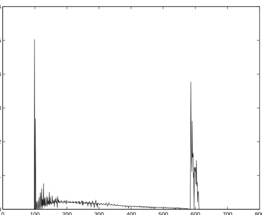
In this section, I calibrate the model to the U.S. data. I let a period be a quarter. I set β = 0.99 so that the annual interest rate is roughly 5%. I set the worker survival rate to be ∆ = 0.995, implying an expected worker life of 50 years. I let v(c)− φ(a) = log(c0 +c)− a0a2, where c, a ≥ 0, and a0 and c0 are positive constants. I assume two output levels so Θ = {θ1, θ2}. I assume X1(a) = exp(−ψa) and X2(a) = 1−exp(−ψa), where ψ > 0. This gives me the following set of free parameters of the model: a0, c0, θ1, θ2, ψ, η. Normalization allows me to set ψ = 1 and θ1 = 0. I set η = 0.6336 so that 63.36% of the population is employed in the model, similar to that in the U.S. data. 20 I then choose a0, c0 and θ2 to target a measure of unemployment of 0.0342 and of a measure of not-in-the-labor-force equal to 0.332. Specifically, by setting a0 = 2.5, c0 = 0.65, and θ2 = 2.75, the model gives a measure of unemployed workers of 0.05031, and the measure of not-in-the-labor-force of 0.31609. In the simulated model, the equilibrium starting expected utility, V, is equal to −0.32932, strictly greater than the worker’s reservation utility
V∗ =−0.33237, as Proposition 10 predicts.
Figure 1 shows the value functions Ur(V) and Uf(V), where the horizontal axis
represents V, the plus signs represent Uf(V) and the dots represent Ur(V). Notice
the worker is terminated (Uf(V) > Ur(V)) if and only V is sufficiently low or it is
sufficiently high. Figure 2 shows the law of motion for the worker’s promised utility
{Vi(V)} where the horizontal axis represents V, the lower curve is V1(V) and the higher curve V2(V). Figures 1 and 2 together indicate that the worker is terminated with probability one after either a sufficiently large number of high outputs or a sufficiently large number of low outputs, regardless of where the employed worker is initially.
Figure 3 shows the worker’s current compensation as a function of his expected utility V and output θ, where the plus signs represent c1(V) and the dots represent
c2(V). Figure 4 shows the worker’s effort as a function of V. Notice the inverted U shape. This is consistent with the idea that the worker is more difficult to motivate when he is too rich or too poor.
For each worker, in the long-run, termination occurs with probability one. This implies an ergodic distribution of promised utilities over a bounded range, following immediately from the fact that the sequence of promised utilities lies in a compact set, so that the cluster points of the sequence constitute the support of the ergodic distri-bution, while the relative frequencies with which each cluster point is hit constitute the ergodic probabilities. One can also establish this result directly by noting that the incentive mechanism constitutes a random walk with reflecting barriers. Figure 5, where the horizontal axis represents the worker’s expected utility, shows the
station-20The Current Population Survey provides monthly data on employment, unemployment and
not-in-the-labor-force, for the period between January 1994 and December 2003. The computed average measures of employment, unemployment, and not-in-the-labor-force are 0.6336, 0.0342, and 0.332, respectively.
ary distribution of the workers: the employed workers in the middle, the unemployed in the left, and the retired in the right.
Consider a new worker starts out with the equilibrium starting expected utility
V. If he produces a low output in the first period, then he is fired immediately. If he produces a high output in the first period, then his current compensation is positive, he is retained and promised a utility strictly higher than V. Suppose in the following periods the worker continues to produce high outputs. Then his expected utility continues to rise, current compensation increases, and he eventually retires with a termination contract that is equivalent to a stream of constant compensation payments. On the other hand, suppose we follow a worker who starts with a relatively high expected utility and produces a sequence of low outputs. Then in each of the following periods, his current compensation is lower, and his expected utility declines, and he is eventually laid off involuntarily.
Consider the relationship between the worker’s wage and his tenure with the firm in the model. From the law of motion for the employed worker’s expected utility that Figure 2 depicts, conditional on a longer tenure at the firm, on average the workers’ expected utility should be higher. As higher expected utilities translate into higher compensations, there is therefore a positive relationship between wage and tenure in the simulated model. The existing literature has provided interesting theories for explaining the observed positive wage-tenure relationship (e.g., Jovanovic 1979; Lazear 1979; Burdett and Coles, 2003; Moscarini, 2005). Unlike mine, these theories are not based on dynamic incentives under private information.
A newer worker faces a higher probability of involuntary lay off than an older worker. Specifically, a fresh new worker is laid off immediately after one low output, as Proposition 13 predicts; whereas it can take many periods of low output before an old worker is fired, depending on where his expected utility is initially. On the other hand, a worker with a longer tenure with the firm (whose promised expected utility is likely to be higher than that of a worker with a shorter tenure) on average has a higher probability to retire and leave the labor force.
Figures 3 and 5 indicate large wage and utility dispersions across employed workers that the model can generate. The stochastic production technology, combined with the mechanism of dynamic incentives and risk sharing, implies that homogeneous workers that start with the same expected utility tend to fan out over time in utility and compensation. This mechanism for generating equilibrium wage dispersion is different from that of the equilibrium search-matching models (e.g., Burdett and Mortensen, 1998; Moscarini, 2003). Hornstein, Krusell and Violante (2006) argue that standard search-matching models can generate only a very small, 3.6%, differential between the average wage and the lowest wage paid in the labor market. 21 This numerical exercise shows that our model has the potential of providing an alternative equilibrium framework for accounting for the observed large wage dispersion.
21The observed Mm ratio–the ratio between the average wage and lowest wage paid– is at least
6
Conclusion
I have constructed and studied an equilibrium model of the labor market where contracts are fully dynamic, job turnover is endogenous, workers terminated from their current jobs are free to go back to the labor market to look for new employment or to stay out of the labor market. The center of the model is an optimal termination mechanism that governs the timing and type of the separation of workers and firms. In equilibrium, this optimal termination mechanism appears in two different faces, involuntary layoff and voluntary retirement.
Compared to the models of efficiency wages and the models of equilibrium search and matching, this paper offers an alternative framework for equilibrium labor market analysis. The contribution to the theory of dynamic contracting is that I model equilibrium multiple transitions between dynamic contracts. An important insight is that termination limits incentive induced inequality.
For my purpose in this paper, I have constructed the model to have a fixed number of jobs. This implies that the demand for labor is fixed in my model. 22 An extension of the model is to endogenize the demand for labor. This can be done by assuming a competitive supply of firms who are free to enter and exit the market, subject to a non-negative cost of staying in operation, as in for example Mortensen and Pissarides (1994); the model is then closed by imposing that the value of entering the market is zero. Obviously, such an extension is not essential for my purpose in this paper. It would not alter any of the qualitative characterizations of the labor market I have presented. In fact, one could simply think of the analysis in this paper as being conditional on the equiliberium number of firms in the more general model with free entry and exit of firms. But such an extension would certainly make the computation and calibration of the model more involved, as well as making the model a better vehicle for quantitative analysis.
7
Appendix
P roof of Lemma1.
For all c ≥ 0, let g[c] denote the termination contract that pays the worker c
units of compensation as long as the worker remains non-employed, and zero once the worker is reemployed. Under this contract, the terminated worker will choose to stay in the labor market if and only if
v(c)−φ(0) 1−β∆ < V ,
22There is also a fixed number of workers in my model, but since the non-employed workers are
allowed to choose whether or not to participate in the labor market, the supply of labor is endogenous in my model.
or c is sufficiently small; otherwise, he will choose to quit the labor market perma-nently. Let cdenote the cut-off level of c that satisfies
v(c)−φ(0) 1−β∆ =V .
Suppose he stays in the labor market, that is, suppose c < c. Then the expected utility he receives from g[c], M(g[c]), is equal to ˆM(g[c]) which solves
ˆ
M(g[c]) =u(c)−φ(0) +β∆(πV + (1−π) ˆM(g[c])).
where remember π(0,1) denotes the probability with which an unemployed worker is matched with a hiring firm, V is the equilibrium starting expected utility of a new worker. Or,
ˆ
M(g[c]) = u(c)−φ(0) +β∆πV 1−β∆(1−π) .
Suppose the worker chooses to quit the labor market, that is, suppose c≥c, then
˜
M(g[c]) = u(c)−φ(0) 1−β∆ . It is straightforward to verify that
ˆ
M(g[c]) = ˜M(g[c]).
Therefore M(g[c]) is well defined, strictly increasing in c with M(g[0]) = V∗ and M(g[∞]) =Vmax. So for anyV ∈[V∗, Vmax) there existsc≥0 such thatM(g[c]) =V.
Q.E.D.
P roof of Lemma 4.
Observe first thatu(0)−φ(0) +β∆V∗ ≤V∗.
I first showV∗ ∈Φ. Notice first thatT U(V) is well defined atV =V∗ becauseUf(·)
is. Second, there cannot be aV such that (V, T U(V)) Pareto dominates (V∗, T U(V∗)),
because T U(V∗)≥Uf(V∗) = maxV0∈Φ
r, V0≥V∗Ur(V
0)≥T U(V), ∀V.
I now prove (i). Let V ∈ [v(0) −φ(0) +β∆V∗, Vmax). Since V∗ ∈ Φ, I can set Vi =V∗ for all i. I then set a = 0, and set ci =c for all i, where c ≥ 0 is chosen to
satisfy the promise-keeping constraint (9). Such chosen{a, ci, Vi}satisfies constraints
(6)-(9). This proves (i).
I now prove (ii). Notice first that V ≥ V∗. Since Ur(·) is concave, (V , Ur(V)) >p
(V, Ur(V)) for all V ∈ [v(0) −φ(0) + β∆V∗, V). Next, by Lemma 3 and equation
(15), I have (V , Ur(V)) >p (V, Uf(V)) for all V ∈ (V∗, V). I therefore have: if V ∈
[v(0) − φ(0) + β∆V∗, V) but 6= V∗, then V 6∈ Φ. To prove the lemma then, it is