Estimation and Control of a Multi-Vehicle Testbed Using GPS Doppler Sensing. Nicholas A. Pohlman

(1)

Estimation and Control of a Multi-Vehicle Testbed

Using GPS Doppler Sensing

by

Nicholas A. Pohlman

Bachelor of Mechanical Engineering, University of Dayton, May 2000

Submitted to the Department of Aeronautics and Astronautics

in partial fulﬁllment of the requirements for the degree of

Master of Science in Aeronautics and Astronautics

at the

MASSACHUSETTS INSTITUTE OF TECHNOLOGY

September 2002

c

The author hereby grants to MIT permission to reproduce and

distribute publicly paper and electronic copies of this thesis document

in whole or in part.

Author . . . .

Department of Aeronautics and Astronautics

September 1, 2002

Certiﬁed by . . . .

Jonathan P. How

Associate Professor

Thesis Supervisor

Accepted by . . . .

Edward M. Greitzer

Professor of Aeronautics and Astronautics

Chair, Committee on Graduate Students

(2)

(3)

Estimation and Control of a Multi-Vehicle Testbed Using

GPS Doppler Sensing

by

Nicholas A. Pohlman

Submitted to the Department of Aeronautics and Astronautics on September 1, 2002, in partial fulﬁllment of the

requirements for the degree of

Master of Science in Aeronautics and Astronautics

Abstract

This thesis presents estimation and control algorithms used to coordinate a multi-vehicle testbed. A total sensor package using the Global Positioning System as the primary sensor with secondary inertial sensors for when GPS is not available and a single point position fix measurement is designed. A new method of integrated velocity estimation is presented using only the Doppler measurements provided by the GPS NAVSTAR constellation. This shows significant improvement on previously used velocity integration methods by elminating unmodeled sensor biases. Furthermore, the algorithm includes the ability to calibrate inertial sensor biases in real-time, which are then used when observability to the constellation is blocked. The single point position fix is able to determine the initial position of the estimation or reset position estimation error drift. Methods are also presented for doing the low-level velocity and heading control of the test vehicle as well as nonlinear closed-loop path following control. Results of multiple estimation algorithms are presented showing that position accuracy with integrated velocity from a coupled GPS/INS/postion fix package is on the order of 10–30 cm over elapsed time of 2–3 minutes. While these errors are larger than CDGPS, the values are lower than typically available from absolute or differential Code phase, and this approach does not have the additional complexity of solving the CDGPS biases. Experiments also demonstrate the robustness and reliability of the path following algorithm. The designed testbed therefore has the necessary estimation and control capability to complete hardware-in-the-loop path following experiments.

Thesis Supervisor: Jonathan P. How Title: Associate Professor

(4)

(5)

Acknowledgments

I would like to thank many people who have helped make this research work a reality. First, to my research advisor Professor Jonathan How, whose insight in both estima-tion and control techniques have helped solve many problems. I appreciate the eﬀort and support to making the testbed work such that it can support future research.

I would also like to thank the many people at MIT who have made this experience educational and enjoyable - Chanwoo Park for initially introducing me to the GPS work and its applications; Many theoretical and social discussions were enjoyed with Arthur Richards, Philip Ferguson, Franz Busse, John Bellingham, Michael Tillerson, and Zachary Traina. I appreciate everyone’s help in carrying equipment back and forth to the outdoor test area.

Lastly, I would like to thank my family for their continuous support. Without their initial push, I would not have enjoyed the academic experience as much as I have. Especially, I would like to thank my wife, Melaine. Through all of the technical detail problems during the research, she helped me keep focused and driven to complete this body of work - forever I am grateful.

(6)

(7)

List of Figures

2-1 Generic GPS receiver tracking loop block diagram [50] . . . 21

2-2 Integer bias between receivers tracking the same transmitter signal . . 24

2-3 Laser position set-up for single point position ﬁx . . . 30

2-4 Rigid body motion of Ellis bicycle model . . . 34

2-5 Cascaded ﬁlters indicated measurements and control inputs to each . 37 3-1 Speed closed-loop control block diagram . . . 44

3-2 Speed closed-loop control response . . . 44

3-3 Heading closed-loop control response . . . 46

3-4 Ground vehicle closed-loop position control . . . 47

3-5 Proportional control model . . . 49

3-6 Autopilot ground track control model . . . 50

4-1 Tamiya Mammoth Dump Truck with electronics payload . . . 58

4-2 Hardware connections for individual truck components . . . 61

4-3 DGPS Velocity Measurements of a Stationary Antenna . . . 62

4-4 Velocity comparison of GPS WLS Doppler solution versus Pendulum speed . . . 63

4-5 Integrated GPS velocity from diﬀerential Doppler measurements . . . 65

4-6 Close-up of start/end of ﬁgure 4-5 . . . 65

4-7 Position results of GPS and Coupled EKF - Run 33 . . . 67

4-8 Area around GPS signal loss and reacq uisition . . . 67

4-9 Close-up of area around single point position ﬁx measurement . . . . 70

(10)

4-14 Multiple autonomous control runs . . . 74

4-15 Final position of control experiments . . . 76

4-16 Final position of control experiment with rotated reference frame . . 76

4-17 Control error of ﬁnal position . . . 77

4-18 Two trucks trading places while avoiding obstacles and collision with one another . . . 78 4-19 Test of dynamic planning algorithm that adjusts plan while maneuvering 79

(11)

List of Tables

1.1 Function of individual measurement device in sensor package . . . 14

2.1 Laser Positioning Error Expectations . . . 32

4.1 Estimation Error Results (m) . . . 73

A.1 Testbed hardware list for ground vehicle . . . 85

A.2 Testbed hardware list for base station . . . 86

A.3 Function keys to change display screen . . . 86

(12)

(13)

Chapter 1

Introduction

This thesis demonstrates the development of a new sensor package and associated estimator incorporating GPS Doppler, inertial navigation sensors (INS) and a single point position ﬁx. The estimation approach will be beneﬁcial for robust high-precision state determination, such as racecar tracking. A new ground vehicle testbed has been created to demonstrate these estimation techniques. This thesis discusses the hard-ware selection for the testbed and presents the low-level control algorithms developed. The overall objective of the constructed testbed is for validation of hardware-in-the-loop advance path planning techniques [53, 55, 56]. Most planning applications are for Unmanned Air Vehicles or autonomous spacecraft maneuvers. The testbed presents a low-cost method for validation. The following subsections discuss each aspect of estimation and control in detail providing motivation and previous research work.

1.1

Precise Estimation

This research investigates the beneﬁts of coupling three measurement systems:

1. GPS Doppler measurements;

2. Onboard vehicle speed and heading measurements; and

(14)

Problem Measurement Device INS GPS Position Fix Integration Drift √ Initial Condition √ Occlusions √

Sensor Biases √

Table 1.1: Function of individual measurement device in sensor package; √ denotes component solving problem

to produce a robust sensor package providing good estimation accuracy with contin-uous updates even with short losses to the precise GPS measurements. Integrating GPS velocity results provides the required position estimation accuracy if continu-ous visibility to signals is maintained. To compensate for signal occlusions due to the environment, an INS system is used to provide measurements when GPS is not available. The coupled filter can use simultaneous GPS/INS measurements to correct the inertial sensor bias errors such that better INS performance is achieved during GPS outages. However, since the filter is based on velocity measurements, there is no direct observation of the position state. The initial position is unknown and the position error drifts during the integration. The addition of a single-point position fix remedies both problems. Table 1.1 shows the components of the sensor package and contribution to the overall filter performance.

During the 1970’s, the United States Air Force began to design a system for a worldwide, all weather navigation system for military maneuvers. After many years of testing and validation, the Global Positioning System (GPS) was oﬃcially activated for civilian use on April 27, 1995 [33]. Using a unique method for signal conditioning, the Navigation Satellite Timing and Ranging (NAVSTAR) constellation accurately provides the measurements necessary for determining precise state estimation.

The purpose of the Global Positioning System is to provide precise navigation solutions in a worldwide reference frame with an accuracy of 1–2 meters [50]. Many applications require more precise state knowledge but in much smaller localized re-gions. Indoor testbeds have been created using specialized local ranging devices [1, 52] such as pseudolites or electromagnetic techniques. The applications of this research

(15)

require larger operating regions than these approaches provide.

Research has shown hardware-in-the-loop precise relative estimation using differ-ential GPS (DGPS) methods [41]. This allows expansion of the operating region for large scale experiments and added precision by eliminating common mode errors in the GPS measurements. But, using carrier-phase differential GPS (CDGPS) can maintain a robust estimation solution only in environments in which full NAVSTAR visibility is continuous [42]. Robustness can be added by using different aspects of the GPS signals, such as differential Code Phase, but the new measurements have significantly higher noise, which degrades the estimation accuracy.

To add robustness to state estimation, backup inertial sensors are included to provide measurements when the GPS signals are unavailable [30, 25]. Previous work has shown simple estimation methods using only INS causes significant state esti-mation error. Typical speed and turning rate integration methods over short time periods (≈ 2 minutes) resulted in 50–100 m position error [10]. Two contributing sources cause the large estimation error. First, measurements from the sensors could simply be wrong due to improper assumptions, such as lateral accelerometers mea-suring gravity when the vehicle is pitched in a turn or wrong wheel radius adding a bias offset to axle encoders. The second significant error source is due to the iner-tial measurements determining states in localized vehicle reference frame. Any error associating the inertial measurement to an external reference frame is unobservable with a stand-alone INS system. Other research uses complementary measurement methods to couple the absolute reference frame measurements (GPS) to those from individual vehicles (INS) thereby reducing overall estimation error [24, 27]. The cur-rent research uses similar coupling methods, however the primary GPS measurement is from Doppler rather than the carrier-phase eliminating solution delay to solve for the CDGPS integer biases.

Many applications may beneﬁt from this robust and precise estimation method. For example, racecar drivers are focused on completing a single lap in the shortest possible time. GPS receivers have shown the capability to solve rapid solutions even in such highly dynamic environments [21]. Accurate tracking of vehicle path enables

(16)

layover comparisons of vehicle performance [16]. By comparing similar instances, vehicle response with respect to input control could be used to compare driving line performance to help train new drivers [15]. Gross errors produced by inexperienced drivers are easily observable with simple sensors. However with precise estimates, enhancements in professional driver performance can be observed therefore oﬀering suggestions for improvement. Additional applications to systems requiring precise state estimation for path control are discussed in the next section.

1.2

Path Following Control

The resulting estimator is used to perform path following closed-loop control. Given the desired state information for steps along the path, the methods presented in this thesis use appropriate controllers to move the vehicle along the path. A nested-loop design is implemented such that low-level controllers complete feedback con-trol on state elements for speed and heading. Outer-loop designs are identified to complete closed-loop position control of individual vehicles. Other work suggests leader/follower fleet path control algorithms such that each vehicle within the fleet was required to continuously follow a manually controlled leader [18]. Closed-loop control in this research can follow a general path provided by any planning algo-rithm. This design enables rapid changes in vehicles or path planning algorithms to validate real-time receding horizon control.

The motivation for the control development is to complete testbed autonomous control maneuvers regardless of the method for path planning. Other applications include precision farming [4], autonomous aircraft landing [12], and Unmanned Air Vehicle maneuvering [45]. In particular, the testbed control can validate high-level control algorithms. Such algorithms have been developed for optimization of vehicle performance [17] and UAV ﬂeet coordination.

(17)

1.3

Hardware Selection

This thesis identifies the components selected for fabrication of the multi-vehicle testbed. Similar testbeds have been developed in the past to test estimation and fleet coordination experiments. For the three-dimensional testbed using blimps [1], experiments were limited to indoor testing facilities, eliminating the possibility of us-ing actual GPS satellite measurements. An outdoor ground testbed usus-ing real GPS equipment was constructed [44], however significant payload weight overloaded the vehicle suspension severely altering the test vehicle dynamic capability. Experimental results were obtained, but reliability of vehicle performance was not acceptable. In this research, a more robust transportation device was selected allowing all of the necessary payload for coordination control experiments to be carried without degrad-ing the vehicle performance. Payload components necessary for sensor measurements, remote control and communication are identified.

1.4

Outline

The following chapters indicate the design and algorithms used to meet the desired objectives of the multi-vehicle testbed. Chapter 2 derives the extended Kalman ﬁl-ter used to produce the reliable and robust estimation algorithm using all available sensors. Control of all aspects of the vehicle, low-level speed and heading as well as path following algorithms, are presented in Chapter 3. The results of many experi-ments of both the estimation and control methods are given in Chapter 4. Finally, Chapter 5 concludes the research objectives achieved in the design and operation of the multi-vehicle testbed and presents future work that can help improve aspects of the new research testbed.

(18)

(19)

Chapter 2

Measurements & State Estimation

This chapter designs the extended Kalman filter used for the vehicle state estimation. Before formulating the specific Kalman filter equations, aspects of the measurement and process model are first introduced.

2.1

Measurement Concepts

This section reviews the construction of GPS signals and presents previous research showing how the signals have be used in similar estimation and control applications. Additionally, the design of the inertial sensors as well as the single position mea-surement system is introduced. Problems of individual systems are identiﬁed and explanations given for how the coupled GPS/INS estimator overcomes these short-comings.

2.1.1

GPS

The original intent of the Global Positioning System was to create a robust naviga-tion tool that could be used to ﬁnd an absolute posinaviga-tion in the worldwide reference frame [33]. Determining position with GPS is done by ranging to separate loca-tions. Consider a range measurement_ρbetween a ﬁxed transmitter _tand user_uwith position vectors being measured from the origin of a coordinate frame, ρt and ρ_u,

(20)

respectively

ρ = ρt−ρ_u (2.1) If the transmitter locations are known, only three measurements are required for a position solution. This section explains how GPS signals are formulated to provide range measurements and transmitter locations thus making it possible to estimate position and/or velocity for any user.

Signal Construction

The GPS signal is a high-frequency, low-power electromagnetic waveform that is being transmitted by the 24 NAVSTAR satellites simultaneously. A standard, inexpensive GPS receiver tracks the repeating Clear/Acquisition Code (C/A-Code), frequency 1.023MHz, being transmitted at the nominal carrier frequency of 1575.42MHz, also known as the L1 band. Signals are also being transmitted for the Precision Code (P-Code) on both L1 and the L2 band, which is at 1227.60MHz. The P-Code has been reserved for military use only, however the C/A-Code and its L1 carrier have proven to be useful for precise relative measurements [33, 34].

The C/A-Code is generated by a pseudorandom number (PRN) digital Code cho-sen from a select number of “Gold Codes” described in Ref. [48]. The 32 particular Codes were selected for GPS use because they have good auto-correlation properties and minimal cross-correlation, both of which are necessary for tracking and locking onto the GPS signal. The PRN Code is then combined with the satellite data mes-sage and the L1 carrier signal to be transmitted. Since each satellite has a unique PRN Code to transmit data, all signals can operate at the same frequency without interfering with one another.

In order to track the signal, the GPS receiver must be able to raise the transmitted signal out of the thermal noise ﬂoor at the L1 frequency. This is accomplished by using the tracking loop diagram shown in ﬁgure 2-1 from Ref. [50]. As shown at the left portion of the tracking loop, replica carrier signal waveforms are generated

(21)

Doppler Measurement

Figure 2-1: Generic GPS receiver tracking loop block diagram [50]

from the onboard oscillator, which then demodulate the input RF signal thereby isolating the PRN Code. Given the speciﬁed 32 PRN codes [35], GPS receivers can replicate the C/A-Code for all transmitting satellites. The receiver quickly slews the current PRN replica across the received signal. Since the cross-correlation of the Gold Codes is very minimal, and the auto-correlation very high, it is easily observed when the two are perfectly correlated. When the peak correlation between signal and replica is found, the receiver can then close the loop to maintain tracking of the C/A-Code. The real-time frequency control to maintain tracking lock on the PRN is the controllable input parameter, more often referred to as Doppler because of the frequency shifting. At a minimum, a GPS receiver reports the replicated Code Phase for all tracked signals as measured on GPS time. Receivers with more advanced communication also provide the carrier phase cycles measured from the beginning of signal acquisition and the Doppler values used in the correlator closed-loop control. It is this Doppler measurement from the GPS receiver that provides very precise velocity measurements for the new estimation method.

Range Measurements

This section discusses the principles for GPS range measurement and discusses why that they are not suitable for our application. The distance between a receiver and the _ith transmitter is calculated by determining the transmission time of the GPS

(22)

signal, commonly referred to as pseudorange (_pr), with the simple model [34]

pri = _c(ˆ_t_k−_t_{satellite transmission})

= ρi −ρ_u+_cτ₀ (2.2) where_cis the speed of light; ˆ_t_k, the receivers current estimate of GPS time;_t_sat_._trans_. is the time tag when the signal left the satellite. For equation 2.2, the range is from equation 2.1 and _τ₀ is the error in the receivers estimate of GPS time. The outgoing satellite signal is synchronized to a standardized NAVSTAR system time determined from very stable onboard atomic clocks. Measuring the elapsed time is a function of distance as well as the accuracy of estimated time onboard the receiver.

Because the waveforms are continuously repeating, the actual measurements pro-vided by the receiver are the accumulated phases _φof the signal. The phase quantity plus the integer number of wavelengths is the actual range between transmitter and receiver. If the integer _β₀ is separated from the total range and included in the mea-surement model, the phase equation, including error sources, for both the Code and carrier phase from the _ith GPS satellite is expressed as [34]

φi = 1 λ (_xi −_x₎2 _{+ (}_yi−_y₎2_{+ (}_zi−_z₎2_/₊ _(2.3) c λ(τ i₋_τ R) +β0i +atmospheric+ν where:

xi, yi, zi = Position coordinates of_ith GPS satellite in an ECEF reference frame

x, y, z = Position coordinates of the receiver in an ECEF reference frame

c = Speed of light

τi = Clock bias of the _ith GPS satellite to actual GPS time

τR = Clock bias of the receiver to actual GPS time

β0 = Integer number of wavelengths between GPS satellite and user at

(23)

= Pseudorange transmission delays due to atmospheric disturbances

λ = Wavelength of tracked signal; 300 km for Code waveform and 19 cm for carrier

ν = Noise on the carrier phase measurement

To maintain the integrity of the system, the satellite locations (_xi_{, y}i_{, z}i_{) and}

indi-vidual clock drifts _τi are precisely monitored and updated by the GPS control center stationed in Colorado Springs and other tracking stations in the global network. To solve for the three elements of the absolute navigation solution as well as receiver clock bias, phase measurements are required from four unique satellites [33].

The accuracy of this absolute position estimation is approximately 1–2 meters when Selective Availability (SA) if oﬀ [50]. (SA was the degradation of GPS time purposely added in order to reduce position accuracy; It was removed from the GPS signals May 1, 2000) [49]. The inaccuracy of the absolute estimate can be traced back to the measurements used to compute the navigation solution. First, errors included in the measurements, such as satellite clock bias and atmospheric delays, are not observable and therefore cannot be eliminated in the estimation ﬁlter. Second, all absolute solutions must use the Code phase measurements rather than the carrier phase, due to the integer bias term _β₀i in equation 2.3. Because Code phase has a much longer wavelength than carrier phase, fewer combinations of the _βi

0 must be

searched to determine the integer wavelengths between the user and transmitting satellite. With the short wavelength of the carrier wave, the carrier bias is impossible to solve in an absolute sense. The Code phase measurement noise is based on the ability to track the 1023 binary chips in the PRN Code. The wavelength of a single chip is ≈300 m thus with 0_.1% tracking accuracy, there is ≈30 cm of noise on each measurement, resulting in the limited navigation accuracy. Conversely, if the carrier phase is tracked with 10% phase accuracy the measurement noise will be ≈ 2 cm making it a better tool for precise estimation.

Because of the short wavelength, carrier phase absolute estimation is nearly impos-sible, thus methods have been developed to use the precise carrier phase for relative estimation. Carrier-Phase Diﬀerential GPS (CDGPS) is formed by taking the single

(24)

x,y,z

x0,y0,z0

Figure 2-2: Integer bias between receivers tracking the same transmitter signal

difference between common satellite phase measurements of two receivers [34]. Differ-ential GPS attempts to eliminate linear common mode errors, such as satellite clock drift and atmospheric delay, from the measurement equation. The differential phase measurement is a function of relative position states and clock biases between two receivers ∆_φi = 1 λ ∆_x2 + ∆_y2+ ∆_z2+ c λ∆τR+β i₊_ν _(2.4)

where (∆_x,∆_y,∆_z) is the relative position vector of the antennas and ∆_τ_R is the relative clock bias between the receivers estimate of time. Note that in equation 2.4, there is a bias term,_βi_{similar to}_βi

0in equation 2.3, representing the integer ambiguity

present in the relative range measurement of the carrier frequency wave, shown in ﬁgure 2-2. The single diﬀerence equation is valid for Code phase measurements as well, thereby improving upon the absolute navigation accuracy, however the large phase measurement noise is still present.

The primary diﬃculty of CDGPS is in that the bias must be re-initialized each time a new measurement is acquired, even after only a brief loss of tracking. Previous research has shown many ways to estimate the measurement integer ambiguity [14]. If the relative position is known exactly, the biases can be determined immediately.

(25)

But, any error introduced by the initial guess causes a slow drift of the position estimation error due to the motion of the GPS constellation. Furthermore, once displacement from the origin occurs, exact bias estimates of newly acquired signals or signals blocked for any period of time cannot be solved. Initializing the carrier phase biases using the initial position method is limited to very short-term applications that maintain continuous sky visibility. Another method to find the ambiguity precisely is to keep all antennas stationary and record the raw tracking data. As the satellites continue on their orbit, the angle of the line-of-sights will change making the integer values observable. The bias is then solved by finding the integer combination that best matches all of the measurements. However, a time delay of 20–40 minutes is often required in order to obtain a sufficient rotation of the NAVSTAR satellites. If a fixed baseline distance between antennas is maintained, the ambiguity can be determined by rotating the antennas to switch locations of the base and remote receivers [5]. Otherwise if the fixed baseline distance is known, a fast integer combination search can be conducted [6]. The benefit of fixed baseline CDGPS estimation is the ability to determine the rigid body attitude in the reference frame. Given the CDGPS solution in the GPS frame, Wahba’s problem [11] can be solved to determine the body frame rotation.

Since most dynamic applications required faster start-up, instantaneous on-the-fly (OTF) procedures have also been developed. Two means for OTF initialization are augmenting the GPS system with a local ranging device or having the receiver track the L2 GPS frequency. Note that both methods typically require a significant increase in equipment costs. Pseudolites that generate exact replicas of the GPS Code can be mounted around the area of use, thereby giving local range measurements without having to add any additional sensing hardware [2, 4, 12]. Rapid changes in the local line-of-sight to the nearby pseudolite can be used to quickly determine the integer biases. Because the pseudolite signal does not contain the standard GPS data messages, the receiver tracking algorithm must be modified to create accurate local ranging measurements. Furthermore, the signal power of the pseudolite must be tuned in order not to inhibit the signals of the GPS satellites from being observable

(26)

to the receiver RF [2]. Also, far ﬁeld assumptions for parallel lines-of-sight are no longer valid and adjustments must be made for the nonlinear eﬀects of the local range measurements for short path initialization [3].

Another option is to use a dual frequency receiver that tracks the L2 band at 1227.60MHz as well as L1. The widelaning technique produces Real-Time Kine-matic (RTK) relative position solutions by measuring the phase of the beat frequency (347.82MHz) of the two bands. This new measurement has a wavelength of≈86 cm, which signiﬁcantly decreases the required integer search space, thus the ambiguity can be solved almost instantaneously [13]. While this method proves to be quick and robust, it typically requires a signiﬁcantly more expensive GPS receiver.

Research has improved methods for integer bias acquisition of L1 band carrier, and once determined, the measurement can provide useful and accurate range information to the estimator. Yet, it has still proven to be difficult when GPS signals are not continuously tracked [42]. Differential Code phase does not have the delayed integer bias acquisition problem, however the pseudorange accuracy is insufficient due to the longer wavelength. Therefore, other available measurements from the Global Position System were considered for the estimator development.

Range Rate Measurements

Rather than focus on new methods for solving integer ambiguity in environments without continuous visibility, this research explores ways to use the Doppler infor-mation to obtain a precise estimate of the velocity of the vehicle. Using the Doppler measurements enables precise estimation immediately after signal lock, thereby elim-inating the delay of integer ambiguity computation. Future sections present methods to create continuous state estimation even during signal occlusion by incorporating backup inertial sensors.

(27)

model to the _ith GPS satellite [41] ˙ φi = 1 λ      ( ˙_xi₋_x_˙₎ ( ˙_yi−_y_˙₎ ( ˙_zi₋_z_˙₎      T       (xi−x) √ (xi−x)2+(yi−y)2+(zi−z)2 (yi−y) √ (xi−x)2+(yi−y)2+(zi−z)2 (zi−z) √ (xi−x)2+(yi−y)2+(zi−z)2      + (2.5) c λ( ˙τ S ₋_τ_˙ R) + ˙+ ˙ν

Equation 2.5 represents the projection (scalar product) of the relative velocity vector between receiver and transmitter (transposed vector on left) onto the vector connect-ing the user to the satellite, more commonly referred to as the line-of-sight (los). The remaining variables, other than position of satellite and user, are the rates of the terms in equation 2.3. The line-of-sight is a unit vector pointing from the absolute position of the user receiver to the absolute position of the tracked satellite. Since the absolute user position is typically available from the pseudorange solution and the ephemeris information of each satellite is transmitted in the GPS data message, the los can easily be formed. Errors of the absolute position solution contribute negligible error to the los calculation. The signiﬁcant diﬀerence that must be noted between equations 2.3 and 2.5 is the elimination of the bias term _βi. Without the delay to determine the bias term, estimation can begin using Doppler measurements immediately after Code phase lock.

In order to reduce common mode errors, diﬀerential Doppler GPS creates the single diﬀerence between two phase rate measurements, user _j and base station_b, to the _ith _{satellite forming}

∆ ˙_φi_j = losi_j•x˙_j,_GPS−losi_b •x˙_b,_GPS+ ∆ ˙_τ + ˙_ν (2.6) where ∆ ˙_τ is the relative clock drift between receivers and x˙ is the vector of velocity components. As indicated previously, the measurement itself is provided from the instantaneous state in the correlator tracking loop ﬁlter. Since typical noise values on these measurements are 0_.5−1_.0 mm/s and primarily white (see discussion in

(28)

Chap-ter 4) a properly formulated ﬁlChap-ter will produce highly accurate velocity estimates with small levels of noise that are primarily white. Given the initial location, the velocity can be integrated for position estimation. A random walk for the position estimation error is generated due to the near-white noise embedded in the velocity estimate. Experiments have shown that, even with the position error drift, estimation using only Doppler measurements provides immediate short-term full state estima-tion with greater accuracy achievable than from diﬀerential Code phase estimaestima-tion. Assuming Code phase accuracy of 1−2 meters and Doppler position estimation drift

≈ 2 mm/s, the Doppler solution will have better performance for up to 10 minutes before reaching diﬀerential Code phase accuracy.

2.1.2

Inertial Systems

In order to add continuous measurement capability to the system, back-up sensors can be included on the test vehicle to provide information when the GPS Doppler measurements are unavailable [30, 28]. Typically, in aerospace applications, these devices have a higher fidelity resulting in significant cost. Research has shown that even low cost sensors can be incorporated into a GPS/INS system to achieve accurate estimation results [25]. This section introduces different inertial measurement sensors and potential errors that contribute to estimation inaccuracy. By using simultaneous measurements from separate devices, estimates of the sensor error can be determined thereby improving the accuracy of the overall system [27].

A wide range of potential sensors such as wheel speed encoders, lateral accelerome-ters, and turning rate gyros could be used to measure variables on the ground-vehicle. In each of the example sensors, the measured quantity is a function of the rates of position or heading. As stated, the motivation for this research is primarily to cre-ate precise position estimation. Previous research has shown that simple integration of these rate measurements over time results in signiﬁcant position estimation error (50–100m) [10]. The current method uses the precise GPS velocity estimate to deter-mine INS sensor errors such that inertial measurements can be improved for operation during short-term GPS signal losses.

(29)

The estimate from GPS sensing solves the relative velocity vector of the user. Therefore, a similar result of measuring speed and heading was desired from the set of INS sensors. The sensor package design was augmented with a wheel axle encoder and a magnetic compass. Assumptions were made about sources contributing to measurement error of the speed and heading. For example, the wheel speed encoder can only be attached to one drive shaft and is affected by tire slip and additional rotation due to the tire having a lateral offset from the center of gravity. Similarly, the compass can be effected by magnetics in the ground vehicle drive motor. Rather than assuming complex measurement models, all errors in the inertial sensors are modeled as additive bias terms. In the filter, the bias states are modeled as integrators driven by zero mean white noise. An estimation scheme that appropriately couples the two measurement capabilities of GPS and inertial sensor is able to determine the steady-state biases in real-time producing a continuous, robust capability while still providing accurate results.

2.1.3

Single Point Position Fix

Accuracy of velocity integration techniques is a function of the precision of the initial position supplied to the system as well as the error drift caused by velocity noise. Ap-plications where similar paths must be compared (i.e. racecar performance) provide a natural position update at the start/ﬁnish line. A limitation is produced, however in that the lateral position of the vehicle cannot be directly determined by breaking a single line. A technique was devised to use two non-parallel laser beams to produce a single point position measurement that can start the integration method or possibly allow a reset of a slowly diverging estimator.

The set-up consists of two transmitting lasers, in our case pen lights, with optical receivers across the path the vehicle traverses. Figure 2-3 shows a schematic indicating the geometric set-up used to determine a single position. The transmitter and receiver locations are denoted by Tand R, respectively. Each time the vehicle breaks a laser beam, the velocity state information (V_1,V₂) from the estimator is stored as well as the elapsed time between beams (∆_T). If a linear change of velocity is assumed

(30)

T

1

T

2

R

V

1

V

2

ρ

₁

ρ

₂ y x +θ

Figure 2-3: Laser position set-up for single point position ﬁx

between the beams, an analytical function can be written for the velocity vector while traveling through the beams

V(_t) = (V2−V1)

∆_T t+V1 (2.7)

where_tis the elapsed time between breaking the two laser beams. When equation 2.7 is integrated from 0 to ∆_T to solve for the traveled path, a constant of integration is introduced S(_t) = V(_t) d_t (2.8) = (V2−V1) 2∆_T t 2₊_V_1t₊_C _(2.9)

The vector constant C is the two-dimensional vehicle position when the ﬁrst laser is broken and located somewhere along the vector connecting the transmitter and receiver. The value of _ρ₁ is the percentage along the vector T₁ −R that the vehicle breaks the beam, hence the initial condition can be produced and substituted into

(31)

equation 2.9 S(0) = _ρ₁(T₁−R) +R (2.10) S(_t) = (V2−V1) 2∆_T t 2₊_V_1t₊_ρ 1(T1−R) +R (2.11)

To solve for the unknown parameter _ρ₁, the terminal condition upon hitting the second beam after an elapsed time of ∆_T must be included

S(∆_T) = _ρ₂(T₂−R) +R

= (V2+V1)

2 ∆T +ρ1(T1−R) +R (2.12)

The resulting vector equation has two unknown parameters,_ρ₁ and_ρ₂. If the receiver locations are set at the origin (R= (0_,0)) and one beam is aligned horizontal to the reference frame (T₁ = (_T₁_,x_,0)) as shown in ﬁgure 2-3, the solution for _ρ₂ collapses to

ρ2 = V2,y+V1,y

2_T₂_,y ∆T (2.13) which can then be substituted into the ﬁnal position constraint in equation 2.12 to determine the positions

  x y   = V2,y+V1,y 2_T₂_,y ∆T(T2) (2.14) If the location of T₂ is created by setting the angle between beams, equation 2.14 can be rewritten as

x = V2,y+V1,y

2 tan_θ_T₂ ∆T (2.15)

y = V2,y+V1,y 2 ∆T

(32)

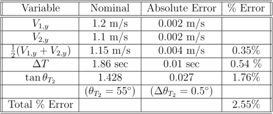
Table 2.1: Laser Positioning Error Expectations Variable Nominal Absolute Error % Error

V1,y 1.2 m/s 0.002 m/s V2,y 1.1 m/s 0.002 m/s 1 2(V1,y+V2,y) 1.15 m/s 0.004 m/s 0.35% ∆_T 1.86 sec 0.01 sec 0.54 % tan_θ_T₂ 1.428 0.027 1.76% (_θ_T₂ = 55◦) (∆_θ_T₂ = 0_.5◦) Total % Error 2.55%

reference frame, the precision of this position update is a function of the accuracy of the velocity estimate at the time of breaking the beam, the accuracy to which ∆_T can be measured and the angle _θ_T₂ between the beam vectors. If the angle of separation is small (_<35◦), the lateral position along the beam vector results in a signiﬁcantly large position measurement error. However, span angles that are too large introduce error in the linear velocity change assumption. Table 2.1 indicates individual variable contributions from equation 2.15 to the position measurement error expected from a typical set-up. The Total % Error can be multiplied by the distance from the receivers that a beam is broken to determine the position accuracy. For cases where the path is less than 1.2 meters away from R, the position error is approximately 3 cm. This expected error can be included in the measurement noise model for the position update so that the ﬁlter does not assume a perfect measurement.

Note, the best position measurement accuracy is achieved closest toR, where the two laser beams meet. If a receiver is created for each transmitter, the lines connecting

T₁-R and T₂-R can be extended to the left such that an × is formed by the laser lines. This enables the area around the intersection to provide greatest position measurement accuracy. The error analysis veriﬁes the expectation of_θ_T₂ to dominate component error contribution to the total error percentage. For improvement of position accuracy, work should focus on methods to improve the knowledge of_θ_T₂.

(33)

2.2

The Extended Kalman Filter

For linear systems, the Kalman Filter produces the optimal recursive ﬁlter for full-state estimation [37, 36]. Updates to the full-state estimate are based on measurements, which often may not provide full state observability, as well as an expected state model. Given a model of the nonlinear vehicle dynamics, expected measurement values can be compared with actual sensor feedback providing a recursive estimate on the full state. An extended Kalman Filter (EKF) is required when propagation and measurement models have nonlinear representation. The models are then linearized when calculating parameters for the Kalman gain and covariance propagation.

The state vector of the designed estimator includes components for position, head-ing, and velocity in a two-dimensional frame relative to a base station reference

x =               N E θ ˙ N ˙ E β               (2.16)

The ﬁrst two elements, (_{N, E}), indicated the north and east positions respectively (with ( ˙_{N ,}_E˙) representing the rates); _θ is the current heading of the rigid body; The

β term indicates those parts of the state vector necessary for measurement model memory, such as previous positions, sensor biases or GPS parameters. Future com-putations will require only the velocity elements of the state vector, therefore the velocity vector V is deﬁned

V =   N˙ ˙ E   (2.17)

(34)

N E L δ +θ V Vehicle Frame longitudinal lateral

Figure 2-4: Rigid body motion of Ellis bicycle model with identiﬁed parameters

2.2.1

Time Propagation

Using a dynamics model, each element of the state can be propagated with a nonlinear function,f, from the previous time step (_k−1) to thea priori estimate at the current time (_k) using the previous statex_k₋₁ and inputs to the system u_k

ˆ

x−_k = f(ˆx_k₋₁_,u_k) (2.18) For rigid body motion of the test vehicle dynamics, the Ellis bicycle model [40] shown in Figure 2-4 was used for the land vehicle with no modeled side-slip. Since our initial application would only be operating at relatively slow speeds, this assumption does not introduce signiﬁcant errors. Individual components of the velocity were created by multiplying the speed by the appropriate trigonometric function of heading

˙

Nk+1 = (V+ ∆uv) cosθ (2.19)

˙

Ek+1 = (V+ ∆uv) sinθ (2.20)

where ∆_u_v is the input parameter for the requested change in longitudinal speed. The value of _θ is zero when aligned with the north vector and increases to _π/2 when aligned directly east creating a North-East-Down reference frame.

(35)

The rate of change of the vehicle heading was modeled by

˙

θk =

V

L tanδ (2.21)

where_Lis the wheel base length of the vehicle and _δ is the turning angle of the front wheels with respect to the vehicle frame, a controllable input.

In order to interpret position information from primarily velocity measurements, a ﬁrst-order Forward Euler integration scheme was used

Nk+1 = Nk+ ˙Nk∆T (2.22)

Ek+1 = Ek+ ˙Ek∆T (2.23)

where ∆_T is the change in discrete time between updates. The covariance matrix _P, an indicator of the reliability of the particular state estimate, is propagated to the a priori value at the current time _P_k− from a linearized calculation

P_k− = _A_k_P_k₋₁_AT_k +_Q_k₋₁ (2.24) where _P_k₋₁ is the covariance from the previous time step and _Q_k₋₁ is the assumed process noise eﬀecting the state. The matrix _A_k is the linear element of the Taylor series expansion of the state propagation equations about the current estimate of the state, x_k Ak = ∂ f(x) ∂x ˆxk (2.25)

The estimator begins with an initial position guess that typically is started from the origin, a surveyed location, or with an erroneous guess to be followed immedi-ately by a position measurement update. Given the testbed vehicle dynamics model, estimates can then be made of the expected measurements from the sensor package and a state update from measurements can be produced.

(36)

2.2.2

Measurement Update

The remaining step of the Kalman ﬁlter is to incorporate the sensor measurements into the current estimate. The set of mathematical equations, h, are a function of state vector elements that create expected sensor measurements

ˆz_k=h(x−_k) (2.26) where ˆz_k is the vector of measurement estimates and x−_k is the a priori estimate from the time update step. Assumptions regarding state element contributions and error sources have been deﬁned and the math models for each of the measurements available from the new GPS/INS sensor package are explained in further detail in future sections.

To create the linear measurement contribution to the Kalman gain _K_k, the vector

h is linearized via the Taylor series expansion to form _H_k

Hk = ∂ h(x) ∂x x−_k (2.27)

Using _H_k, Kalman ﬁlter gain is computed

Kk = Pk−HkT(HkPk−HkT +Rk)−1 (2.28)

where _P_k− is the a priori time updated covariance of the state vector and _R_k the measurement covariance matrix (_R_k = _E[_ννT_{]). Given the} _{a priori} _{state estimate}

ˆ

x−_k, actual measurementsz_k, the expected nonlinear measurementsˆz_kand the Kalman gain _K_k the measurement update of the state can be completed

ˆ

x_k = ˆx−_k +_K_k(z_k−ˆz) (2.29) as well as the necessary state covariance updates from the current measurements

(37)

GPS

EKF

Coupled

EKF

N,E,

θ

∆Φ

u

_k

z

_INS

x

Figure 2-5: Cascaded ﬁlters indicated measurements and control inputs to each

The accuracy of the sensors as well as the measurement models eﬀect the results of the extended Kalman Filter.

Note, to make the measurements of the velocity vector and heading from GPS available for comparison with the INS measurements, two filters were cascaded using synchronized measurements but the same time propagation equations. A schematic of the estimator design is shown in figure 2-5. The control inputs, _u_k are supplied to the time propagator of each filter. The GPS EKF uses all of the available differential Doppler measurements, ∆ ˙Φ, from the GPS receivers. The Coupled EKF uses INS measurements, _z_INS, and GPS velocity results, ˙_{N ,}_{E, θ}˙ , to continuously compute a state estimate,xˆ. Separate filters enabled a comparison of GPS methods alone, GPS methods with backup INS measurements and INS methods alone. The following sections identify the measurement models used for each filter.

GPS Measurement Model

Recall that for diﬀerential Doppler methods, the relative velocity between two users (_j and _b) is a measure of the projected velocity vector of each user onto their respective

los vectors to the _ith common satellite

∆ ˙_φi_j = losi_j•x˙_j,_GPS−losi_b •x˙_b,_GPS+ ∆ ˙_τ + ˙_ν

If it is assumed that the satellites are far enough away and that the receivers are close enough together (_< 5km) that the los vectors are virtually parallel such that

(38)

equation 2.6 can be reduced to the form

∆ ˙_φi_j = losi_b•∆ ˙x_j,_GPS+ ∆ ˙_τ+ ˙_ν (2.31) The measurements are range rates in the relative reference frame. Typically, the base receiver is stationary to maintain a static reference for the Doppler measurement. Therefore, the relative measurement is a function of the actual precise velocity of the remote vehicle. Stacking _N measurements together into a single vector ∆ ˙Φ, substituting the correct elements of the state vector and creating the corresponding geometry matrix_Gfrom the transposedlosvectors forms the linear algebraic equation

∆ ˙Φ =         los1T 1 los2T 1 .. . losNT 1                 ˙ N ˙ E ˙ D ∆ ˙_τ         + ˙_ν (2.32) ≡ G 1         ˙ N ˙ E ˙ D ∆ ˙_τ         + ˙_ν

where ˙_D is the relative vertical velocity of the ground vehicle and ∆ ˙_τ is the relative clock drift rate. These two parameters are necessary to formulate the problem, but are of no interest to the current estimation result, therefore they are included as elements of the vector β in the state. In the second line of equation 2.33, the _Nx3 matrix _G is concatenated with the vector of ones on the right hand side creating the linear measurement matrix_H_{GP S}. Typically 6–10 satellites are visible from surface of the earth, each providing range rate information in the direction of the line-of-sight. After the estimate of the total velocity vector is updated, a GPS heading can be

(39)

formed by taking the four quadrant arctangent of the velocity components [7] θGP S = arctan ˙ E ˙ N (2.33)

The value _θ_{GP S} as solved from equation 2.33 follows the heading measurement con-vention of (0_,2_π) at north and increasing clockwise from above. However, the mea-surement is only useful when the vehicle is in motion.

Coupled Measurement Model

For the sensor bias estimation in the Coupled EKF, the precise North and East velocity results of the GPS estimation are supplied as measurements

z_{E,GP S}˙ = E˙ +ν_{E,GP S}˙ (2.34)

z_{N ,GP S}˙ = N˙ +ν_{N ,GP S}˙ (2.35)

The output of the GPS ﬁlter is an assumed unbiased velocity measurement in the N-E reference frame. Most linear factors that introduce errors are eliminated by using a single diﬀerence measurement.

The GPS heading measurement is supplied to the coupled ﬁlter assuming no contributing error sources besides white noise

zθ,GP S = θ+νθ,GP S (2.36)

Errors could be caused by side-slip of the ground vehicle. Research has shown that CDGPS methods with two antennas attached to a test vehicle can observe the dif-ference between vehicle heading and velocity [42]. The constructed testbed showed no side-slip eﬀects through any dynamic control therefore it was determined that the complexity of using more hardware and expanding the estimation would not be worth the beneﬁt.

(40)

constel-lation visibility and able to track at least 4 signals. If GPS velocity and heading measurements are not supplied to the coupled ﬁlter, the vector of expected measure-ments ˆz_couple and the linearized matrix _H_couple are reduced in size accordingly.

As mentioned in section 2.1.2, a compass measurement was used as the backup sensor when in a stationary position or during GPS signal occlusion. The measure-ment was assumed to include the actual value of the heading _θ as well as a constant bias due to magnetic disturbances (i.e. the drive motor on the RC truck)

zθ,IN S = θ+βθ+νθ,IN S (2.37)

The _β_θ term was added as another state vector element. During simultaneous mea-surements of GPS and the compass, the bias can be estimated and later used to correct the compass measurement at times when INS must operate alone.

To determine the path distance traveled during a time step, an encoder is attached to an axle of a rear wheel. The path divided by the wheel radius _r generates a representation of the rotation of the wheel axle

zs,IN S = (

(_N_k−_N_k₋₁)2+ (_E_k−_E_k₋₁)2+_β_s)_r−1+_ν_{s,IN S} (2.38) Because of possible error in the radius measurement and/or because the actual path was laterally offset for the rigid body center of gravity, the bias term _β_s was used to model the error of the encoder measurement. As with the compass, the bias term can be estimated during simultaneous GPS/INS measurements and can be used to correct the measurement while using INS alone. Equation 2.38 assumes a straight-line path connecting the previous position estimate, _k−1, to the current value, _k. A higher fidelity model could include a curvilinear path that uses change in heading as well as position. In the case of this research development, the measurement update periods are sufficiently short (nominally available at 5 Hz) such that the straight-line assumption appears to work well.

If the vehicle passes through the laser set-up described in section 2.1.3, a single position measurement can be input to the ﬁlter. All of the previous formulations exist

(41)

with the additional condition of the position measurement

zN = N +νN,GP S (2.39)

zE = E+νE,GP S (2.40)

It was assumed that no additional biases were observable in the position measurement and all measurement error (see table 2.1) was incorporated into the noise.

The parameters shown in the coupled measurement model equations not already present in the state vector (_N_k₋₁_{, E}_k₋₁_{, β}_θ_{, β}_s) were concatenated to become part of

β. Constants were assumed for all of the parameters therefore resulting in no changes due to dynamic propagation.

Note that the primary measurements observe the rate elements of the state vector. The measurement limitation causes the position covariance to drift to larger values as the ﬁlter progresses forward in time. When using CDGPS, the position covariance quickly converges to provide precise state estimation regardless of elapsed ﬁlter time. In the case when GPS Doppler is used, the position covariance grows very slowly. For the short term applications used in this research, the drift rates are small enough to achieve good position accuracy but any situation requiring long estimation time will have much better position error results with CDGPS.

Due to larger expected noise values of the inertial sensors, the covariance drifts much faster when only INS is available. The only improvement of position covariance is through the laser beam position update where the measurement model quickly reduces the position covariance over one step providing some increased conﬁdence in the position state estimate. Essentially, all of the previous position state information is eliminated and the measurement update causes a noticeable jump in the estimated path (see results in Chapter 4).

(42)

2.3

Estimation Conclusions

By included estimated sensor errors in the measurement model, the integrity of the total GPS/INS sensor system could be improved when GPS signals are unavailable or if blocked. If greater bandwidth is desired for dynamic observability of the overall filter, the frequency of the INS could be significantly faster than that of GPS. Updates on the bias estimation would then be limited to only those times when both measure-ment capabilities were available. For the current application, the INS measuremeasure-ment system was to be used to augment the robustness of the GPS velocity estimation algorithm. Results of the designed filter are presented in chapter 4.

(43)

Chapter 3

Vehicle Control

While the estimation methods are important for state determination, the overall ob-jective of creating an autonomous ﬂeet of roving vehicles requires development of algorithms to perform two-dimensional vehicle control. It is assumed that a set of path waypoints is supplied to each vehicle in the testbed requesting speciﬁc maneu-vers. The formulation of the path is beyond the scope of this thesis and can be found in Ref. [45]. The motivation for vehicle control is to validate hardware-in-the-loop ex-periments of real-time path planning. A nested-loop control architecture is designed. This chapter discusses the low-level control of speed and heading for the ground ve-hicle. It concludes with algorithms to create reference inputs of heading and speed to complete closed-loop path-following control.

3.1

Speed Control

The forward motion of the test vehicle hardware is driven by a digital input. This value is passed to a micro-controller which converts to a pulse width modulated (PWM) signal that drives a servo. This then turns a potentiometer arm which drives the DC motor voltage. (Actual components and manufacturers are identiﬁed in Ap-pendix A).

The closed-loop control system block diagram is shown in ﬁgure 3-1. The plant was modeled as a ﬁrst-order lag with 1–2 second time constant. A lead-lag compensator

(44)

sensor Process Noise 1 T.s+1 Plant L P Gain Measurement Noise s+2 s+5 Lead-Lag Controller 1 s Integrator V Esitmator V Constant

Figure 3-1: Speed closed-loop control block diagram

0 10 20 30 40 50 60 0 0.1 0.2 0.3 0.4 0.5 0.6 0.7 0.8 0.9 1 Time (sec) Speed (m/s) Reference Speed Measured Response

Figure 3-2: Speed closed-loop control response

with integral action is employed. The ﬁnal compensator design is a pole at -5 and a zero at -2. The overall proportional gain of the controller _L was tuned high enough to produce fast response of the system. However, consideration was taken to be sure the value was low enough that control would not request input saturation even at maximum closed-loop error.

Because the measurements are made at discrete times, the actual algorithm is pro-grammed using digital control techniques, with a zero-order hold on a 5 Hz sampling rate [38]. Figure 3-2 indicates the controller performance, ×, for a constant input reference speed (solid line). Fast response to the step input is observed with an over-shoot of speed. Some oscillation in the response is expected since the compensator design produced closed-loop poles oﬀ of the negative real axis. Longitudinal speed

(45)

disturbances are caused by side-slip of the front steering wheels and undulations in the surface. The results in ﬁgure 3-2 indicate the mean error is only 0_.036m/s with a standard deviation of 0_.069m/s. These results are satisfactory for closed-loop control of longitudinal speed for the ground vehicle testbed.

3.2

Heading Control

The rigid body heading is controlled by steering the front wheels with servos, per the Ellis bicycle model [40]. The heading rate equation 2.21 from the dynamics model in section 2.2.1 indicates the plant for heading control is nonlinear

˙

θk =

V_k

L tanδ

Another contributing factor not included in equation 3.1 is an actuation saturation limiting of _δ to ≈ ±20◦. When operating around the linearized region, the plant can be modeled as a ﬁrst-order lag. This can be stabilized by a proportional controller.

Separate control gains, _K_r and _K_l, were deﬁned for positive and negative error to compensate for the non-uniform response of the left/right turning mechanism. Similar to the speed control gain, the value was set high enough that the response time would be 1–2 seconds given a step input (∆_{θ >} 25◦). An upper limit on the gain was determined in order not to force the controller to immediately approach the mechanical saturation limits. All of the nonlinear factors contributed to a minimum turn radius of ≈2m (maximum ˙_θ≈75−85◦/s) for the ground vehicle.

Further consideration was also made for the phase-wrap of the heading that occurs at 0 and 2_π. It was assumed that the minimum and maximum bound of the heading error could be ±_π, respectively. By forcing the error bounds, diﬀerences around the nonlinear wrap point would not result in vehicle control commanding an entire circle to be traversed.

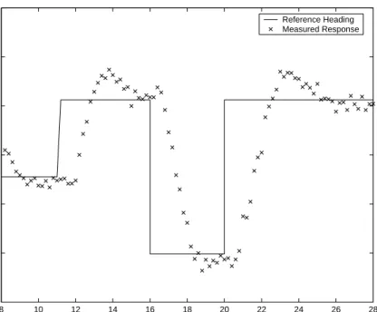
Figure 3-3 shows the performance of the closed-loop controller with large step changes of the reference heading. The response and settling time met the control

(46)

8 10 12 14 16 18 20 22 24 26 28 −1 −0.5 0 0.5 1 1.5 2 Time (sec)

Heading Angle (radians)

Reference Heading Measured Response

Figure 3-3: Heading closed-loop control response

requirements (∆_θ_ref = 45◦ at 11 s; −90◦ at 16 s; and 90◦ at 20 s). Under typical op-eration, the reference heading has a more continuous change ( ˙_{θ <}20◦/sec), resulting in better tracking of the closed-loop heading control.

3.3

Position Control

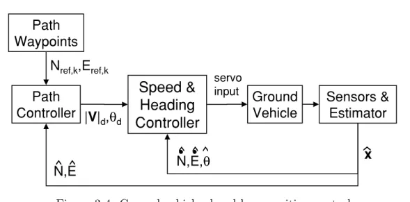
With the low-level controllers designed, an outer control loop was developed to use the two desired inputs (V_d_{, θ}_d) to create a nested-loop feedback control system, shown in ﬁgure 3-4. The outer-loop performance hinges on the satisfactory control of the speed and heading states by the low-level feedback loop. This section presents outer-loop control designs used to complete the position control requirement.

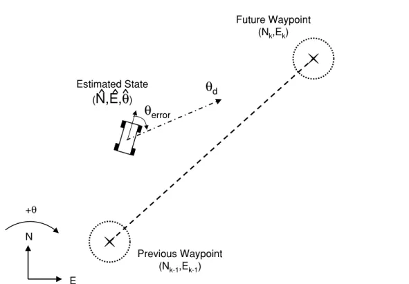
It is assumed that all planned paths supplied to the testbed provide waypoint locations, as well as all components of the state vector. The desire is not only to reach a particular location, but to reach the location with a desired heading such that a continuous smooth path may be traveled. The actual path trajectories were designed using receding horizon control with mixed-integer linear programming [45]. The path planning method is able to consider dynamic constraints such as a nominal

(47)

Path

Waypoints

x

Ground

Vehicle

Speed &

Heading

Controller

Sensors &

Estimator

Path

Controller

N,E

N,E,

θ

N

_ref,k

,E

_ref,k

|

V

|

_d

,

θ

_d servo input

Figure 3-4: Ground vehicle closed-loop position control

constant speed and minimum turn radius such that the formulated paths are within the vehicle dynamic capability. Feedback of the completed path can also be provided to the path generation algorithm to determine if a new plan must be designed and executed to meet the overall objectives.

3.3.1

Heading provided by plan

In this control scheme, the speed and heading references are taken directly from the plan synchronized to GPS time. Assuming that the low-level controllers were able to create dynamic performance equal to the model used for planning, the resulting motion would naturally generate the requested path. To maintain a smooth change in heading between waypoints, the control computer used a linear interpolation between the current heading direction and the desired future heading

θd=θk−1+ (θk−θk−1)

ˆ

t−tk−1

tk−tk−1

(3.1)

where_θ_k₋₁is the heading at the previous achieved waypoint; _θ_kis the desired heading at the next target location; ˆ_t is the current estimate of GPS time; _t_k₋₁ and _t_k are the planned times when the vehicle should be at the previous and future waypoints, respectively. Once again, care must be taken when desired headings from the plan cross the phase wrap of the vehicle heading. Nominally, the absolute diﬀerences in

(48)