DP
RIETI Discussion Paper Series 07-E-003
Estimation Procedures and TFP Analysis
of the JIP Database 2006 (Revised)
FUKAO Kyoji
RIETI
INUI Tomohiko
Nihon University
Hyeog Ug KWON
Nihon University
MIYAGAWA Tsutomu
Gakushuin University
TOKUI Joji
Shinshu University
HAMAGATA Sumio
Hitotsubashi University
ITO Keiko
Senshu University
MAKINO Tatsuji
Hitotsubashi University
NAKANISHI Yasuo
Senshu University
RIETI Discussion Paper Series 07-E-003 First draft: January 2007
Revised: June 2007
Estimation Procedures and TFP Analysis of the JIP Database 2006
Kyoji Fukao Hitotsubashi University Sumio Hamagata Hitotsubashi University Tomohiko Inui Nihon University Keiko Ito Senshu University Hyeog Ug Kwon Nihon University Tatsuji Makino Hitotsubashi University Tsutomu Miyagawa Gakushuin University Yasuo Nakanishi Senshu University Joji Tokui Shinshu University June 2007
Introduction
The purpose of this paper is to explain the preliminary version of the newly compiled Japan Industrial Productivity Database (JIP 2006) and report some results of our growth accounting analysis based on this database. The JIP 2006 contains information on 108 sectors from 1970 to 2002 that can be used for total factor productivity analyses. These sectors cover the whole Japanese economy. The JIP Database was compiled as part of the RIETI (Research Institute of Economy, Trade and Industry) research project “Study on Industry-Level and Firm-Level Productivity in Japan.” The original version of the JIP Database (ESRI/Hi-Stat JIP Database 2003) was compiled in a collaboration between ESRI (Economic and Social Research Institute, Cabinet Office, Government of Japan) as part of its research project on “Japan’s Potential Growth” and Hitotsubashi University as part of its Hi-Stat project (A 21st-Century COE Program, Research Unit for Statistical Analysis in the Social Sciences).1 The authors are grateful to ESRI and members of the Hi-Stat team for the support and cooperation provided for our present RIETI project.
At this moment, the major data available are sectoral capital service input indices and labor service input indices, including information on real capital stocks and the nominal cost of capital by type of capital and by industry, the nominal and real values of sectoral gross output and intermediate input, as well as some supplementary tables, such as statistics on trade, inward and outward FDI, and Japan’s industrial structure. All real values are based on 1995 prices. For growth accounting, nominal labor costs and nominal capital services for 108 industries are also estimated. The sum of these two values for each industry is not adjusted to be equal to the value added of that industry at factor cost base.
The final version of the JIP 2006 is scheduled to be released by August, 2006. The final version will include nominal and real annual input-output tables, detailed information on ICT capital services and some additional statistics, such as R&D stocks and capacity utilization rates at the detailed sectoral level.2
For scholars familiar with the JIP 2003, we here briefly summarize the main differences between and the main similarities of the 2006 and 2003 versions of the JIP.
1. The JIP 2003 is based on the 1968 SNA, while the JIP 2006 is based on the 1993 SNA. The capital stock of the JIP 2006 includes order-made software, plant engineering, and assets accumulated by the search for minerals. The JIP 2003 uses SNA statistics as control totals. Following Japan’s present SNA statistics, capital stock in the preliminary version of the JIP 2006
1 Details on the old version of the JIP database (JIP 2003) can be found in Fukao, Inui, Kawai, and Miyagawa (2004). The JIP 2003 is downloadable at
http://www.esri.go.jp/en/archive/bun/abstract/bun170index-e.html . 2 The present preliminary version of the JIP 2006 is available at
does not include prepackaged and in-house software. However, the final version of the JIP 2006 will include two sets of statistics, one in which capital stock does not include prepackaged and in-house software and one in which it does.
2. In the case of the JIP 2006, labor input data include detailed information on labor input cross-classified by categories of labor.
The paper is organized as follows: In the next section, we report the estimation procedures of our annual input-output tables. In Sections 2 and 3, we explain the capital service input data and the labor input data of the JIP 2006, respectively. Finally, in Section 4, we analyze Japan’s sectoral and macro TFP growth.
1. Estimation of Annual Input-Output (IO) Tables 1.1. Sectoral Classification
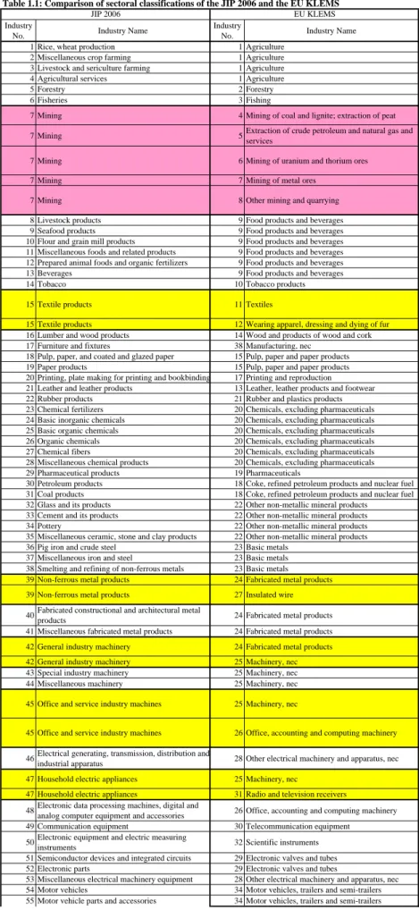
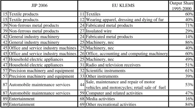
Following the principle of the IO tables of Japan’s Ministry of Internal Affairs and Communications (MIC; formerly: Management and Coordination Agency (MCA)), the sectoral classifications of the JIP 2003 and of the JIP 2006 are on an activity (commodity) basis, not on an industry basis. Compared with the JIP 2003, which classifies activities into 84 sectors, the JIP 2006 classifies activities into 108 sectors. The sectoral classification of the JIP 2006 thus is much more detailed, especially in the machinery and information service sectors. Using the 4-digit level concordance between the International Standard Industrial Classification (ISIC), Rev. 3.0, and the Standard Industrial Classification for Japan (JSIC), 2002 Revision, Table 1.1 compares the 108 sectors of the JIP 2006 with the 72 industries of the EU KLEMS project, which is on an industry basis and not on an activity basis. Table 1.2 shows the correspondence of the two classifications for selected sectors.
1.2. The Compilation Procedures of the JIP IO Tables
For the estimation of nominal and real IO tables (the latter in 1995 prices) at the most detailed level of the JIP 2006 classification, we used three types of IO tables compiled by the Japanese government.
Every five years, a relatively reliable, linked IO table is available. Therefore, we chose the years 1970, 75, 80 85, 90, 95 and 2000 as our benchmark years. Major data sources for our annual IO tables for the benchmark years are:
1970-1975-1980 Linked IO Tables, MCA; 1980-1985-1990 Linked IO Tables, MCA; 1985-1990-1995 Linked IO Tables, MIC;
1990-1995-2000 Linked IO Tables, MIC;
For other years before 1999, we used the annually compiled Extended IO Tables published by the Ministry of Economy, Trade and Industry (METI; formerly: Ministry of International Trade and Industry (MITI)). For the years after 2001, we used the annually compiled SNA IO Tables published by the Cabinet Office (CAO).
There are some differences in the concepts and methods of compilation underlying the above-mentioned IO tables and we adjusted for these. Physical capital in the lease industry, which is rented to other industries, is treated as capital input in the lease industry. The cost of R&D in each sector is included in the production cost of that industry. The JIP Database is based on the 1993 SNA. Therefore, software investment is included in investment. Depreciation of government capital is included in the consumption expenditure of the government.
Next, we constructed converters to make adjustments for changes in industry classifications over time and aggregated the IO data into our 108 sectors.
We compiled IO tables in real terms (in 1995 prices) in the following way. The 1970-1975-1980 Linked IO Tables contain real IO tables at 1980 prices. Similarly, the 1980-1985-1990 Linked IO Tables contain real IO tables at 1990 prices. We linked these two real IO tables at year 1980. The second and the third IO statistics are linked at year 1990. The third and fourth IO statistics are linked at year 1995.
As control totals of gross output and intermediate input at more aggregated sectoral classification levels, we used the Matrix on Output of Goods and Services Classified by Economic Activities (V Matrix) and the Matrix on Input of Goods and Services Classified by Economic Activities (U Matrix) of CAO.
In the future, we could use these V and U Matrices to convert the JIP 2006 IO Tables on an activity basis into EU KLEMS-type IO tables on an industry basis.
It is important to note that the values in the JIP IO tables are measured at producer prices, while the EU KLEMS IO tables are measured at basic prices. Using data on indirect taxes, subsidies and tariffs by commodity as well as the intermediate input matrix of imported commodities, the Research and Statistics Department of the Economic and Industry Policy Bureau at METI is now trying to convert the Basic Transaction Table of the 2000 IO Tables of the MIC valued at producer prices into a table at basic prices. Once we have obtained their results for 2000, we will start to do the same for other years.
2. Capital Stock Data of the JIP 2006 Database
industry and by capital good in the JIP 2006 database. We estimate the net capital stock for 1970 and use this as the benchmark figure. We then estimate capital stock for 1970 to 2002, using the perpetual inventory method. This method makes use of annual investment series by industry and by capital good and of a constant depreciation rate for each category of capital stock.
All real series are valued at 1995 prices. Our database consists of 108 industries based on Japan’s Input-Output Tables. Capital goods are classified into 39 capital goods categories in our database. We call our own classification of industries and capital goods the “JIP 2006 (Japan Industry Productivity) classification.”
Our capital stock database covers not only the private sector but also public enterprises and government services. In addition, it contains data on residential stocks.
2.1. Outline of the Construction of Capital Stock Data
We construct capital stock data following the five steps outlined below. Step 1: Choice of coverage of capital stock
Our capital stock data cover the following five sectors: (1) the private corporate sector (including personal firms); (2) the public corporate sector; (3) the non-profit organization sector; (4) the government sector (education, health, sanitary services, etc.); and (5) the household sector (owner-occupied housing).
Step 2: Classification of industries and estimation of capital formation series by industry
We distinguish 107 industries based on the Fixed Capital Formation Matrix (FCFM) of the Input-Output Tables of Japan. While the JIP 2006 database has 108 industries, we do not estimate capital formation for the last category, “activities not elsewhere classified.” Following Fukao et al. (2004), we obtain capital formation data by industry from the FCFM. Because the FCFM data are published only every five years, we estimate the data for intervening years by interpolating and using other data sources that contain annual investment data.
Step 3: Estimation of capital formation series by asset
We estimate capital formation series by asset using the method in Fukao et al. (2004). We distinguish 39 assets, following the classification of the Bureau of Economic Analysis (BEA) of the United States.
Step 4: Estimation of real capital stock by industry and by asset
Adjusting control totals in capital formation series by industry and by asset, we estimate capital formation series by industry and by asset for every year, using the RAS method. In addition, we
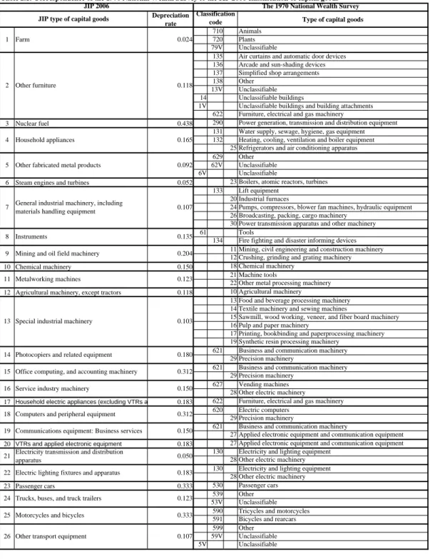
construct a benchmark capital stock matrix fromthe 1970 National Wealth Survey (1970 NWS). By using capital formation series by industry and by asset, the benchmark capital stock matrix for 1970, and investment deflators (normalized at 1995 prices) by asset, we construct capital stock series by industry and by asset from 1970 to 2002.
Step 5: Estimation of the measure of capital services
Because we construct a multi-asset capital stock database, we consider capital services as a production factor, following Jorgenson and Griliches (1967). Assuming that the marginal productivity of capital asset j is equal to the cost of capital of asset j, we construct a Divisia-index for capital services using the ratio of the value of asset j to the total asset value as a weight.
The following subsections provide a more detailed explanation of the construction of the capital stock database.
2.2. Estimation of Capital Formation Series
We estimate the capital formation series from 1970 to 2002 by industry and by asset. Classifications of industries and assets are based on the JIP 2006 classification.
2.2.1. Estimation of Capital Formation Series by Industry
Because capital formation data by industry are published every five years and we cannot construct the annual capital formation data from FCFM, we have to interpolate annual capital formation data for intervening years by using other surveys. For the manufacturing sector, we use the Census of Manufactures, which is published annually. For the non-manufacturing sector, we construct the annual capital formation data by using industry-specific surveys and balance sheet data of public enterprises. Because these data are based on sample surveys and do not cover all establishments in each industry, we estimate annual capital formation series by industry by adjusting the annual capital formation by industry to the capital formation data in the FCFM.
This is the basic procedure we have tried to follow in principle. However, for some sectors or periods, it was not possible to follow this procedure, because, especially in the 1970s, the sectoral classification of the FCFM is rougher than that of the JIP. In cases where one FCFM sector comprises several different sectors of the JIP 2006 classification, we apportion the data according to the proportion of production of each sector given in the Input-Output Tables. This is exactly the same procedure as the one we employ to calculate the 1970 benchmark stock.
2.2.2. Estimation of capital formation series by asset
We estimate the capital formation series by asset following Fukao et al. (2004). We rearrange these data using the JIP 2006 asset classification.
As for intangible assets which were not included in the JIP 2003, we note that our database covers only custom software (asset classification No. 38 of the JIP 2006) and plant engineering (asset classification No. 39 of the JIP 2006) in accordance with Japan’s 93 SNA. To estimate these investment series, we use the Survey of Selected Service Industries published by the Ministry of Economy, Trade and Industry.
2.2.3 Estimation of the fixed capital formation matrix for every year
The above-mentioned estimation procedures provide us with a capital formation matrix which is by industry and by asset. However, we have a fixed capital formation matrix only for every five years. We therefore estimate the fixed capital formation matrices for the intervening years using the FCFM and the RAS method.
2.3. Estimation of benchmark capital stock data for 1970
We construct the benchmark stock by industry and by capital good based on the 1970 National Wealth Survey (1970 NWS). In this section, we describe how we transform the original data to fit the JIP classification.
2.3.1. Outline of the 1970 National Wealth Survey
National Wealth Surveys were conducted every five years from 1955 to 1970. As the 1970 NWS is the most comprehensive and most recent survey, we use this as our starting point. The characteristics of the 1970 NWS are as follows.
First, it relies on capital asset data collected from eight types of institutions and economic agents: the central government, local governments, central government enterprises, local government enterprises, incorporated enterprises, non-profit organizations, unincorporated enterprises, and households. Second, the 1970 NWS is constructed based on the 68 SNA. Third, capital asset data for nine regional areas in Japan are available. Fourth, all capital assets are arranged in terms of their owners and users. Fifth, the 1970 NWS distinguishes between new and second-hand capital goods.
All land, natural resources, and financial assets are excluded from this survey. It covers only reproducible tangible fixed capital goods.
For the JIP 2006 database, we use all the data that are available by industry and by capital asset, except for inventory capital goods, social overhead capital and household durable goods. The dataset is on an ownership-basis, including purchases of second-hand goods.
2.3.2. Estimation of benchmark capital stock data for 1970
We construct the benchmark stock by industry and by capital asset based on the 1970 NWS. We transform the original data to fit the JIP 2006 classification using the following process:
First, because the 1970 NWS statistics are in terms of firms and organizations, while the FCFM underlying the JIP 2006 data is based on production activities, we transform the original data in the 1970 NWS into activity-based data by applying the rate of distribution of each capital good to every industry in the FCFM for 1970.
Second, we need to bring the very different sectoral and capital asset classifications of the 1970 NWS into line with those of the JIP. For example, the JIP 2006 classification system has 108 industries and 39 capital goods, while the 1970 NWS has 26 industries and 54 capital goods. We conduct our reclassification using the detailed information on output and employment from the Census of Manufactures.
Third, all capital assets, including second-hand assets, in the 1970 NWS are valued at 1970 prices. Thus, we need to rebase the original data using 1995 prices. The value of capital goods is deflated using the 1995 price indices for capital assets which are calculated following the method used by Fukao et al. (2004).
Fourth, in the 1970 NWS, the public sector is surveyed at the end of the 1970 fiscal year. We therefore convert the data on the public sector for 1970 into calendar-year data.
2.4. Construction of real net capital stock for 1970-2002
The fixed capital formation series estimated following the methodology described in Section 2.3. are in nominal terms. We convert the series from nominal to real terms using 1995 prices. We use deflators following Fukao et al. (2004).
Next, using the capital stock for 1970 as the benchmark figure, we cumulate capital stock using the perpetual inventory method. This means we have to consider the depreciation of the capital stock. To do so, we assume a constant depreciation rate for each capital good, which we take from the BEA. The depreciation rate for each capital good is shown in Table 2.1.
(Insert Table 2.1)
2.5. The construction of capital input and quality indices
Because we construct a multi-asset capital stock database, we consider capital services as a production factor. Following Jorgenson and Griliches (1967), to construct an index of capital input for sector i (Vi(t)), we assume the marginal product of capital is equal to the rental price of capital.
The translog quantity index for sector i is calculated as follows:
(
, 1)
[
ln () ln ( 1)]
) 1 ( ln ) ( lnV t − V t− =∑
S t t− Kij t − Kij t− j ij i i , (2.1)where Kij(t) stands for the capital stock of capital good j in sector i and the weights are defined as the
(
)
[
() ( 1)]
2 1 1 ,t− = S t +S t− t Sij ij ij , and∑
= j ij ij ij ij ij u t K t t K t u t S ) ( ) ( ) ( ) ( ) ( .The rental price of capital services for capital good j in sector i uij(t) is described as follows.
]
)
1
(
)
1
(
)
(
)
(
)
(
)
(
))
(
1
))(
(
1
)[(
(
)
(
1
)
(
1
)
(
j j j j i i i j i ij ijt
p
t
p
t
p
t
r
t
b
t
i
t
b
t
h
t
p
t
h
t
z
t
u
+
δ
−
−
−
−
+
−
−
−
−
=
,where pj(t) is a price of good j. hi(t) is the corporate tax rate in sector i. i(t) is nominal interest rate.
We get the data obtained from long-term bonds issued by the Japanese government. r(t) is long-term loan rate obtained from the statistics from Bank of Japan. bi(t) is the debt /asset ratio in sector i. We
get the data of bi(t)from Financial Statement Survey of Enterprises surveyed by Ministry of Finance.
δj is depreciation rate of asset j and is time-invariant. zij(t) is the present value of depreciation
deductions on investment of 1 yen and calculated as follows:
]
)
(
)
(
)
(
))
(
1
))(
(
1
[(
)
(
)
(
j i i i j i ijt
r
t
b
t
i
t
b
t
h
t
h
t
z
δ
δ
+
+
−
−
=
.Next, we define the change in the capital quality index (QiK(t)) as the difference between the
change in capital input and that in the unweighted sum of capital stock of capital good j in sector i: ) 1 ( ) ( ln ) 1 ( ) ( ln ) 1 ( ) ( ln − − − = − Z t t Z t V t V t Q t Q i i i i K i K i , (2.2) where
∑
= = 39 1 ) ( ) ( j ij i t K t Z .2.6. An Overview of Capital Stock and Quality Indices
We now look at some of the major trends in the data we constructed. Table 2.3 shows the real net capital stock by industry in Japan. The aggregated capital stock in Japan was 236 trillion yen in 1970. Since then, it has grown by 5.7 % per annum, reaching 1,483 trillion yen in 2002. The ratio of the real capital stock in manufacturing industries to that in all industries was 19.5 % in 1970. It subsequently gradually declined to 14.4 % in 1985 and in recent years has been stable at around 15 %.
Table 2.2 displays the growth rate of capital stock in each industry. It shows that the growth rate has gradually declined and was only 0.9 % in the period 2000-2002 due to the collapse of the
information and communication technology (ICT) bubble. In the manufacturing sector, the growth rate was 1.5 % for the period 1995-2000 and -0.2 % for the period 2000-2002. Capital stock grew faster in the non-manufacturing sector than in the manufacturing sector during these periods.
When we look at the growth rate of capital stock by industry, we find that the growth rate in ICT industries is relatively high. In the manufacturing sector, it was particularly high in “semiconductor devices and integrated circuits” (JIP 2006 industry classification No.51) at 10.3% per annum and in “electronic data processing machines, digital and analog computer equipment and accessories” (JIP 2006 industry classification No. 48) at 10.0 % per annum.
In the non-manufacturing sector, “rental of office equipment and goods” (JIP 2006 industry classification No. 86) and “information services and internet-based services” (JIP 2006 industry classification No. 91) displayed the highest rates of growth in capital stock with 13.9 % and 13.3 %, respectively.
(Insert Table 2.2)
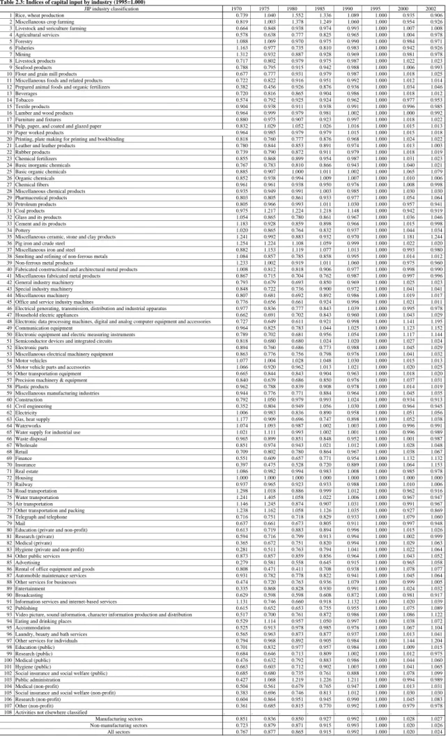
Indices of capital input by industry are shown in Table 2.3. The capital input indices of ICT industries such as “information services and internet-based services” (JIP 2006 industry classification No. 91) and “semiconductor devices and integrated circuits” (JIP 2006 industry classification No. 51), grew rapidly during the period 1980-1990. On the other hand, in the 1990s, it was non-manufacturing industries such as “advertising” (JIP 2006 industry classification No. 85) and “broadcasting” (JIP 2006 industry classification No. 90) that showed high growth rates.
(Insert Table 2.3)
2.7. Capital formation and capital stock in information and communication technology (ICT) goods
Following the guidelines of the OECD regarding information and communication capital, we select ICT capital assets from 39 assets in the JIP 2006 and construct ICT capital formation and ICT capital stock series by sector. Table 2.4 provides our classification of ICT capital assets in the JIP 2006. Because the JIP 2006 follows the coverage of Japan’s 93 SNA, own-account software and prepackaged software are not included in our definition of ICT capital assets.
(Insert Table 2.4)
Aggregate ICT investment in Japan increased by 10.0% per annum between 1970 and 2002 (Figure 2.1), substantially faster than the average growth rate of total investment (2.3%). The ratio of
ICT investment to total investment increased from 2.4% in 1970 to 23.9% in 2002.
(Insert Figure 2.1)
Figure 2.1 shows that the rapid increase in investment in computer and peripheral equipment and custom software was the main factor behind the increase in aggregate investment. One important reason for the increase in computer and peripheral equipment investment was the rapid decline in prices. In addition, growing investment in hardware, along with outsourcing by firms, contributed to the increase in software investment.
However, recent ICT investment in Japan does not show a monotonic growth trend and appears to have been cyclical. In the first half of the 1990s, aggregate ICT investment declined temporarily because investment in “other ICT tangible assets” decreased as a result of the collapse of the bubble economy. In contrast, the second half of the 1990s witnessed a veritable boom in ICT investment. However, the end of ICT boom in the U.S. induced a decline in investment in computer and peripheral equipment which contributed to the downturn in aggregate ICT investment.
The ICT capital stock also increased rapidly. In 1970, the ICT capital stock at 1995 prices was only 3 trillion yen, but this reached 128 trillion yen in 2002. As shown in Figure 2.2, the ICT capital stock grew at a rate of 12.5% per annum from 1970 to 2002. The ratio of the ICT capital stock to total capital stock increased from 1.2% in 1970 to 8.6% in 2002.
(Insert Figure 2.2)
3. Estimation of Labor Input 3.1 Overview of the estimation
We have constructed indices of labor input for each industrial sector in the Japanese economy based on the methodology developed by Gollop and Jorgenson (1980). These are Divisia-indices constructed from data on hours worked (i.e., man-hours) and labor compensation cross-classified by the sex, age, education, and employment status of workers.
Table 3.1 shows our breakdown of labor input characteristics. With respect to the employment status, workers are classified into three categories: (1) full-time wage and salary workers, (2) part-time wage and salary workers, and (3) self-employed and unpaid family workers.
An annual classification by education group consistent with our database is available only for full-time wage and salary workers. Therefore, full-time wage and salary workers for each industry are cross-classified by sex, eleven age groups, and four education groups, while other workers are cross-classified only by sex and eleven age groups.
(Insert Table 3.1)
Data on the number of workers, hours worked, and labor compensation cross-classified like this are not readily available. We have therefore combined several data sources and used the RAS method as well as other procedures to compile them.
Our data sources consist of both household surveys such as the Population Census, the Employment Status Survey, and the Labour Force Survey, and establishment surveys such as the Establishment and Enterprise Census, the Monthly Labour Survey, and the Basic Survey on Wage Structure.
When measuring the number of workers, household surveys and establishment surveys count multiple-job holders differently. While household surveys do not double-count workers even if they have a second job, establishment surveys do double-count these workers. In order to construct measures of labor input that are consistent with Japan’s SNA, we adopt the practice of double-counting workers with a second job.
In constructing the other measures of our database, such as output, intermediate input, and capital, we distinguish different activities even at the establishment-level. In order to construct labor input indices consistent with these measures, we therefore have to distinguish labor input for different activities at the establishment-level as well, since many establishments produce multiple products. To bring the labor data in line with the activity-based measures, we use the detailed V-table (the establishment-activity table) of Japan’s SNA.
3.2. The Number of Workers
We start our estimation of the number of workers using the data provided by the Population Census. Since the Population Census does not double-count second-job holders, we also use the Employment Status Survey, which asks households about household members’ work status and whether they hold second jobs. We use this information to add the number of workers with second jobs to the number of workers from the Population Census. As both of these surveys are conducted every five years, we estimate annual data of the number of workers based on the Population Census using the information of the annual Labour Force Survey, and linearly interpolate the number of workers with second jobs provided by the Employment Status Survey.
Thus, we obtain three sets of marginal totals of the number of workers cross-classified by two characteristics: (a) sex×employment status (wage and salary worker, and self-employed and unpaid family worker), (b) sex×age, and (c) sex×industry (at the one-digit industry level).
Iteratively applying the RAS method to the above three sets of marginal totals, we obtain the number of workers cross-classified by four characteristics: sex×employment status (wage and salary
worker, and self-employed and unpaid family worker)×age×industry (at the one-digit industry level). The next step is to disaggregate the number of workers by the finer industry classification. To obtain the information for this step, we rely on many different data sources: the Statistical Yearbook of the Ministry of Agriculture, Forestry and Fisheries, the Statistical Survey on Farm Management and Economy and other statistics for agriculture, the Employment Table of the Input-Output Tables for construction, the Census of Manufactures for manufacturing, and the Establishment and Enterprise Census for other industries.
To divide wage and salary workers into full-time workers and part-time workers, we define part-time workers as those whose average number of hours worked in a week is less than 35. Using the information from the Labour Force Survey, the Employment Status Survey, the Basic Survey on Wage Structure, and the Establishment and Enterprise Census, we count the number of part-time workers cross-classified by sex×age×detailed industry classification. Subtracting the number of part-time workers from that of all wage and salary workers, we obtain the number of full-time wage and salary workers.
As mentioned above, we classify full-time wage and salary workers by education group. To obtain the information on these workers’ educational background, we rely on the Basic Survey on Wage Structure.
The number of workers counted and cross-classified as above is consistent with the number of workers counted by Japan’s SNA. However, when we add up our estimated numbers to the aggregation level of the SNA, there are small but almost constant discrepancies between them. To adjust for these discrepancies, we calculate adjustment coefficients and multiply our estimated numbers by them.
3.3. Hours Worked
To measure the average hours worked by full-time wage and salary workers, we use the data from the Monthly Labour Survey as benchmark data. The data on average hours provided in the Monthly Labour Survey are the sum of both actual hours worked within scheduled hours and overtime hours worked. However, these data are available only for the low dimensional cross-classification, sex×one-digit industry classification. In order to obtain the data on average hours worked by age group, educational attainment, and detailed industry classification, we use the information from the Basic Survey on Wage Structure.
For the average hours worked by part-time wage and salary workers, we use the information on the average hours worked by female part-time wage and salary workers from the Basic Survey on Wage Structure. Since these data are classified by the relatively broadly defined one-digit industry, we assume that the average hours worked in the same broadly defined industry are not different. In addition, since we only have data on female part-time workers, we assume that the average number
of hours worked by male part-time workers is the same as that for female part-time workers.
In order to measure the average hours worked by self-employed and unpaid family workers, we use the following procedure. First we calculate the ratio of the average hours worked by self-employed workers and by full-time wage and salary workers, using the Labour Force Survey. These data are cross-classified by sex×one-digit industry classification. The average hours of full-time wage and salary workers cross-classified by age, educational attainment, and detailed industry classification are multiplied by the above ratio to obtain the average number of hours worked by self-employed and unpaid family workers cross-classified in the same way.
Since agriculture, forestry and fisheries, and government services are not covered by the Monthly Labour Survey and the Basic Survey on Wage Structure, we use the average hours worked in these industries from the Labour Force Survey as benchmark data In order to obtain data cross-classified by age and education, we calculate the average hours worked in construction, manufacturing, and transportation and communication based on the Basic Survey on Wage Structure and use this as supplementary information for agriculture, forestry and fisheries. In the same way, we use the average hours worked in service industries as supplementary information for government services.
3.4. Labor Compensation
As benchmark data for estimating the labor compensation of full-time wage and salary workers, we use the Monthly Labour Survey. Since the Monthly Labour Survey data cover only wages and salaries actually paid, we adjust them using the General Survey on Working Conditions in order to obtain labor compensation including not only cash payments but also other labor expenses. We use the Basic Survey on Wage Structure to take differences in wage rates and other labor compensation by sex, age, educational attainment, and detailed industry classification into account.
For the labor compensation of part-time wage and salary workers, we use data on female part-time workers from the Basic Survey on Wage Structure. We apply the same wage rates to both sexes and to workers in industries belonging to the same major industry.
In order to measure the labor compensation of self-employed and unpaid family workers, we adopt the following procedure. First we calculate the ratio (γi(t)) between self-employed workers’
income and wage and salary workers’ income using the Employment Status Survey, which provides data cross-classified by sex, and the broadly defined one-digit industry. The labor compensation of wage and salary workers (wiE(t)) cross-classified by age, educational attainment, and detailed
industry classification is then multiplied by the above ratio (γi(t)) to obtain the average
self-employed workers’ income (γi(t)×wiE(t)) cross-classified in the same way.
After estimating the part of a self-employed worker’s income that should be imputed to the capital share, we can subtract it from his/her total income to obtain his/her labor compensation.
Therefore, the average labor compensation of self employed worker (wiS(t)) is given by
( )
t(
( )
t)
( ) ( )
t w t w E i i i S i = 1−α* γ (3.1)where αi*(t) denotes the industry’s capital income share. On the other hand, the capital share αi*(t) is
given by the following equation:
( )
( ) ( )
( ) ( )
t K t w( ) ( )
t L t w( ) ( )
t L t u t K t u t S i S i E i E i j ij ij j ij ij i = + +∑
∑
* α (3.2)where uij(t), Kij(t), LiE(t), and LiS(t) denote the rental price of capital services, real capital stock,
man-hours of full-time and part-time workers, and man-hours of self-employed workers respectively. The above two equations have two unknown variables, wiS(t) and αi*(t). Substituting (3.1) into
(3.2), we obtain the quadratic equation of αi*(t). In case that this quadratic equation has two solutions
for αi*(t), one solution takes a value between zero and one, and the other solution is larger than one.
Hence, we can throw away the latter solution to obtain only one relevant solution, which is given by the following equation (the abbreviated symbol “t” for time is omitted in this equation):
S i E i i j ij ij S i E i i S i E i i E i E i j ij ij S i E i i E i E i j ij ij i L w K u L w L w L w K u L w L w K u γ γ γ γ α 2 4 2 *
∑
∑
∑
⎟⎟ − ⎠ ⎞ ⎜ ⎜ ⎝ ⎛ + + − + + = (3.3) Finally, by substituting the value of αi*(t) into (3.1), we get wiS(t).3.5. The Construction of Labor Input and Quality Indices
We have explained the construction of data on annual number of workers, average hours worked, and average labor compensation per hour for each industrial sector. These data are cross-classified by the sex, age, education, and employment status of workers. Following Gollop and Jorgenson (1980), in constructing the Divisia-index of labor input for sector i (Li(t)), we assume that sectoral
labor input Li(t) can be expressed as a translog function of each category’s man-hours MHij(t). The
Divisia quantity index for industrial sector i is constructed as follows:
(
, 1)
[
ln () ln ( 1)]
) 1 ( ln ) ( lnL t − L t− =∑
S t t− MHij t − MHij t− j ij i i . (3.4)In the above equation, MHij(t) stands for the man-hours of category j workerin industrial sector i at
time t and the weights are given by the average share of the labor compensation for each category j worker in the total value of sectoral labor compensation:
(
)
[
() ( 1)]
2 1 1 ,t− = S t +S t− t Sij ij ij , and∑
= j ij ij ij ij ij w t MH t t MH t w t S ) ( ) ( ) ( ) ( ) ( ,where wij(t) denotes the labor compensation for category j worker in industrial sector i at time t.
Since the labor input index Li(t) constructed as above takes the differences of compensation per
hour among workers classified in different categories into account, it reflects differences in labor quality among differently classified workers. Therefore, we can construct the labor quality index by taking the difference between the growth rate of the labor input index and that of the unweighted sum of hours worked in each industrial sector. Hence, the growth rate of the labor quality index (QiL(t)) in industrial sector i can be expressed as:
) 1 ( ) ( ln ) 1 ( ) ( ln ) 1 ( ) ( ln − − − = − MH t t MH t L t L t Q t Q i i i i L i L i , (3.5) where
∑
= =128 1 ) ( ) ( j ij i t MH t MH .3.6. Changes in Labor Input at the Sectoral Level
Average annual growth rates of sectoral labor input indices are presented in Table 3.2 for seven subperiods between 1970 and 2002 for 107 industries. Although in each decade, we find industries in which labor input increased or decreased, the increase in labor input in expanding industries in the 1990s was relatively slow when compared with the 1970s or 1980s. Another notable development is that almost all the industries in which labor input increased during the 1990s were in the service sector, which is in stark contrast with the 1980s, when many of the industries in which labor input increased hailed from the manufacturing sector.
(Insert Table 3.2)
Table 3.3 and Table 3.4 show, respectively, the average annual growth rates of sectoral man-hours and labor quality indices in the same way as Table 3.2. We can observe a gradual slowdown in the rise in labor input quality in many industries.
(Insert Tables 3.3 and 3.4)
Man-hours, labor input indices, and labor quality indices can each be aggregated into broadly defined sectors such as manufacturing, non-manufacturing, and the economy as a whole. Man-hours are simply added, while the methodology of aggregating labor input indices is described in Section
4.2.1. As for labor quality indices, we calculate the growth rate of the labor quality index by taking the differences between the growth rate of the aggregated labor input index and aggregated man-hours.
Trends in the major indicators – the number of workers, man-hours, and the labor input index – aggregated for the economy as a whole are shown in Figure 3.1. As can be seen, the number of workers only began to decrease in 1998. In contrast, man-hours already started to decline at the beginning of 1990s. The reason is the shortening of working hours promoted by the Japanese government at that time. Finally, the labor input index remained fairly stable until the mid-1990s and since then has been declining much more slowly, reflecting continuing improvements in labor quality. However, compared with the 1970s and 1980s, when the labor input index was growing much more rapidly than man-hours, improvements in labor quality also appear to have slowed down in the 1990s.
(Insert Figure 3.1)
Trends in labor input indicators for manufacturing and non-manufacturing industries are shown in Figures 3.2 and 3.3. In the manufacturing sector (Figure 3.2), labor input declined in the early 1970s, but then steadily increased again during the second half of the decade and throughout the 1980s. However, since the early 1990s, labor input in the manufacturing sector has been declining rapidly. In contrast, in the non-manufacturing sector (Figure 3.3), labor input grew steadily until the mid-1990s and has been stagnating since.
(Insert Figures 3.2 and 3.3)
A decomposition of the average annual growth rate of the labor input indices of each of the 52 manufacturing industries for the period 1970 to 2002 is provided in Figure 3.4. While there are a number of manufacturing industries in which labor input increased over these three decades, most saw a decrease. The direction of change in labor input in each industry is largely determined by the change in the number of workers, which grew in some but shrank in others. In contrast, the number of hours per worker declined across the board and to a very similar degree. On the other hand, although labor quality also increased across the board, there are considerable differences in the degree of increase. The most successful industries were the IT-related sectors, which show a relatively high increase both in the number of workers and labor quality.
Figure 3.5 provides a decomposition of the average annual growth rate of labor input indices for each of the 55 non-manufacturing industries. As illustrated in the figure, there are many service industries in which labor input increased, but also a few industries, particularly in the primary sector, where labor input diminished. Again, most of the change in labor input is explained by changes in the number of workers. Improvements in labor quality only made a small contribution to overall labor input.
(Insert Figure 3.5)
As the above considerations have shown, changes in labor quality have played only a minor (though not negligible) role in explaining changes in labor input overall. On the other hand, the changes in the labor quality index reflect changes in the composition of the different components of the labor force. Hence, we take a brief look at changes in the composition of the labor force. Notable changes in the composition of the labor force over the past three decades can be observed.
Tables 3.5, 3.6, and 3.7 show the ratio of female workers, of part-time wage and salary workers, and of workers aged over fifty-five in each of the 107 industries in the years 1970, 1980, 1990, and 2000. Looking at the trends indicated by these tables, we find that the ratio of female workers has risen gradually in many industries. Industries showing exceptions to this trend are those in the electrical machinery sector, where the ratio of female workers peaked in the mid-1980s and has been declining since. Another notable trend is the increase in the ratio of part-time wage and salary workers. In recent years, part-time wage and salary workers have come to account for more than ten percent of all workers in almost all industries. The ratio of older workers has also increased notably, reflecting the aging of Japan’s society. Workers over fifty-five now account for more than twenty percent of the work force in many industries.
(Insert Tables 3.5, 3.6, and 3.7)
4. Growth Accounting at the Sectoral and the Macro Level
In this section, we analyze the sources of sectoral and macroeconomic output growth. Moreover, we derive the growth of total factor productivity (TFP) in each industry and in the macroeconomy.
4.1. Growth Accounting at the Sectoral Level
Our methodology of decomposition is based on the economic theory of production. The economy is divided into I sectors producing I different commodities. Gross output in sector i in period t is assumed to be produced with a production function using various types of input [capital
(V1,…,Vk), labor (L1,…,Ll) and intermediate commodities (M1,…,Mm)]. Ai(t) is an indicator of the
state of technology.
( )
t A t F(
V( )
t V( ) ( )
t L t L( )
t M( )
t M( )
t)
Yi = i()⋅ 1i ,L, ki , 1i ,L, li , 1i ,L, mi (4.1)
We assume that this function is separable in such a way that the various types of capital, labor and intermediate inputs may be aggregated into indices Vi(t), Li(t) and Mi(t), respectively, so that we
may write the production function as:
( )
t A t F(
V( ) ( )
t L t M( )
t)
Yi = i()⋅ i , i , i (4.2)
The index of capital input is derived by the aggregation of several types of assets, structures, and equipment. The labor input index is an aggregate of the number of workers cross-classified by sex, age, employment status, and educational attainment. The material input index is derived by the aggregation of the 108 commodities.
We assume that the production function exhibits constant returns to scale; that firms minimize the costs of inputs, subject to the production technology shown above; and that factor input markets are competitive. Equation (2) can then be differentiated by time and manipulated as follows:
( )
t S( )
t d V( )
t S( )
t d L( )
t S d M( )
t d A( )
t Ydln i = Vi ln i + Li ln i + Mi ln i + ln i (4.3)
where dlnYi(t)=lnYi(t)-lnYi(t-1),dlnVi(t)=lnVi(t)-lnVi(t-1),dlnLi(t)=lnLi(t)-lnLi(t-1),
dlnMi(t)=lnMi(t)-lnMi(t-1), and the S
( )
t 's are the two-period average shares of the subscripted inputin the total cost.
( )
[
( )
( )
1]
21 + −
= S t S t t
SVi Vi Vi : the two-period average capital input cost share
( )
[
( )
( )
1]
21 + −
= S t S t t
SLi Li Li : the two-period average labor input cost share
( )
[
( )
( )
1]
21 + −
= S t S t t
SMi Mi Mi : the two-period average material input cost share
It is difficult to measure and observe the state of technology Ai(t) but it is easy to measure the
contribution of technological change to production in the following way:
( )
t d Y( )
t[
S( )
t d V( )
t S( )
t d L( )
t S( )
t d M( )
t]
Adln i = ln i − Vi ln i + Li ln i + Mi ln i . (4.4)
most industries experienced a slow-down in TFP growth during the 1990-2002 period when compared with earlier periods. Figure 4.1 shows each industry’s TFP growth rate in the period 1970-2002. This figure shows that there was a wide variation in TFP growth among industries.
4.2. Growth Accounting at the Semi-Macro and the Macro Level
We can also decompose output growth at a more aggregated level, such as the manufacturing sector, the non-manufacturing sector and the total economy. In order to aggregate input and output at the industry-level to the sectoral level, we apply the chain-linked or Divisia-index method as discussed below, in order to take account of yearly changes in each industry’s share in total sectoral production. In addition, we use Laspeyres-type quantity measures of output, value added and material inputs for the decomposition of output growth.
4.2.1. Aggregation of Labor Input
We define each variable as follows:
L(t): The sum of labor input indices from industry i to industry n in period t. Li(t): The labor input index in industry i in period t.
MHij(t): The total annual number of hours worked by category j worker in industry i in period t.
wij(t): The average hourly wage for category j worker in industry i in period t.
The aggregated labor input L(t) can subsequently be calculated using the following formula:
( )
−( )
− =∑
n(
−)
[
( )
−( )
−]
i i i L i t t L t L t S t L t L ln 1 , 1 ln ln 1 ln , (4.5) where( )
( )
( )
( )
∑∑
∑
= n i m j ij ij m j ij ij L i t MH t w t MH t w t S () and(
)
[
( ) ( 1)]
2 1 1 ,t− = S t +S t− t S L i L i L i .4.2.2 Aggregation of Capital Input
We define each variable as follows:
V(t): The sum of capital input indices from industry i to industry n in period t. Vi(t): The capital input index in industry i in period t.
Kij(t): The amount of capital stock of capital good j in industry i in period t.
uij(t): The capital cost for category j capital good stock in industry i in period t.
The growth rate of the aggregated capital input V(t) can then be calculated using the following formula:
( )
−( )
− =∑
n(
−)
[
( )
−( )
−]
i i i V i t t V t V t S t V t V ln 1 , 1 ln ln 1 ln , (4.6) where( ) ( )
( ) ( )
∑∑
∑
= n i m j ij ij m j ij ij V i t K t u t K t u t S ( ) and(
)
[
() ( 1)]
2 1 1 ,t− = S t +S t− t S V i V i V i .4.2.3. Divisia-Index Type of Aggregation of Real Output
We define each variable as follows:
Y(t): The sum of real gross output values from industry i to industry n in period t. Yi(t): The real gross output value of industry i in period t.
NY(t): The sum of nominal gross output values from industry i to industry j in period t. NYi(t): The nominal gross output value in industry i in period t.
The growth rate of the aggregated gross output Y(t) can then be calculated using the following formula:
( )
−( )
− =∑
n(
−)
[
( )
−( )
−]
i i i Y i t t Y t Y t S t Y t Y ln 1 , 1 ln ln 1 ln , (4.7) where(
)
( )
( )
( )
( )
⎥⎦ ⎤ ⎢ ⎣ ⎡ − − + = − 1 1 2 1 1 , t NY t NY t NY t NY t t SYi i i .4.2.4. Divisia-Index Type of Aggregation of Real Input Values
We define each variable as follows:
M(t): The sum of real material input values from industry i to industry n in period t. Mi(t): The real material input value in industry i in period t.
NM(t): The sum of nominal material input values from industry i to industry j in period t. NMi(t): The nominal material input value in industry i in period t.
The growth rate of the aggregated gross output M(t) can subsequently be calculated using the following formula:.
( )
−( )
− =∑
n(
−)
[
( )
−( )
−]
i i i M i t t M t M t S t M t M ln 1 , 1 ln ln 1 ln , (4.8) where(
)
( )
( )
( )
( )
⎥⎦ ⎤ ⎢ ⎣ ⎡ − − + = − 1 1 2 1 1 , t NM t NM t NM t NM t t SiM i i .4.2.5. Laspeyres-Type Chain-Linked Index for Real GDP
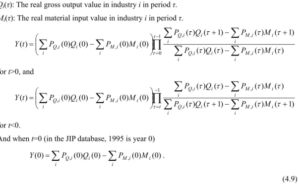
We can define real GDP as the differencebetween the Divisia-index type of aggregated gross output and that of material input as outlined above, but this method does not have additive consistency. Hence, we calculate the output of the economy as a whole (total value added) by applying a Laspeyres-type chain-linked index, as shown below.
We define each variable as follows:
Y(t): The real value added in the total economy in period t.
PQ,i(τ): The product price index of industry i in period τ (1995 prices).
PM,i(τ): The material price index of industry i in period τ (1995 prices).
Qi(τ): The real gross output value in industry i in period τ.
Mi(τ): The real material input value in industry i in period τ.
∏
∑
∑
∑
∑
∑
∑
− = − + − + ⎟⎟ ⎠ ⎞ ⎜⎜ ⎝ ⎛ − = 1 0 , , , , , , ( ) ( ) ( ) ( ) ) 1 ( ) ( ) 1 ( ) ( ) 0 ( ) 0 ( ) 0 ( ) 0 ( ) ( t i Mi i i Qi i i i i M i i i Q i Mi i i Qi i P Q P M M P Q P M P Q P t Y τ τ τ τ τ τ τ τ τ for t>0, and∏
∑
∑
∑
∑
∑
∑
− = + − + − ⎟⎟ ⎠ ⎞ ⎜⎜ ⎝ ⎛ − = 1 , , , , , , ( ) ( 1) ( ) ( 1) ) ( ) ( ) ( ) ( ) 0 ( ) 0 ( ) 0 ( ) 0 ( ) ( t i Mi i i Qi i i i i M i i i Q i Mi i i Qi i P Q P M M P Q P M P Q P t Y τ τ τ τ τ τ τ τ τ for t<0.And when t=0 (in the JIP database, 1995 is year 0)
∑
∑
− = i i i M i i i Q Q P M P Y(0) ,(0) (0) ,(0) (0). (4.9)4.2.5. Growth Accounting at the Macro and the Semi-Macro Level
Using these aggregated output and input indices, we can also decompose output growth at the aggregate sector level, such as manufacturing, non-manufacturing, and the total economy, by applying formula (4.4). The results of the decomposition using the chain-linked or Divisia-index type output and material inputs are shown in Tables 4.1, 4.2, and 4.3. Here, we further decompose the labor input and capital input growth rates into their quantity and quality growth rates. We also use Laspeyres-type quantity measures of value-added gross output and material inputs for the decomposition of output growth, and the results are displayed in Tables 4.4, 4.5 and 4.6.
Table 4.1 shows the TFP growth rate in the total economy in each sub-period. The TFP growth rate slowed down substantially in the 1990-2002 period when compared with previous periods. The
annual average TFP growth rate fell to almost zero in the 1990-1995 period, but slightly recovered to around 0.4% in the 1995-2002 period. The contribution of labor quality growth to output growth is fairly stable and positive in the whole period, but there was a large decline in the contribution of man-hour growth in the 1990-2002 period.
As can be seen in Table 4.2, the TFP growth rate in the manufacturing sector is similar in the 1970-1980 and the 1980-1990 period. However, in the 1990-2002 period, the TFP growth rate declined by 0.74 percentage points from that witnessed in the 1980-1990 period. In addition to the slowdown in TFP growth, man-hour growth and the contribution by capital input also declined in the 1990-2002 period, and all three of these factors together explain the large decline in output growth during 1990-2002.
In the non-manufacturing sector, the TFP growth rate was somewhat positive in the 1970-1980 period, but then became negative in the 1990-2002 period (see Table 4.3). As in the manufacturing sector, the slow-down in TFP growth was exacerbated by slower growth in man-hours and capital inputs, which all contributed to the slower output growth during 1990-2002.
Appendix: Supplementary Tables
The main part of the JIP 2006 consists of industry-level data on capital stock and labor input, input-output tables, etc., which can be used for total factor productivity analyses. This Appendix provides a brief explanation of supplementary tables that can be used to examine the determinants of sectoral productivity growth. The supplementary tables, which are preliminary, include the following: (1) trade in goods by industry and country; (2) inward and outward FDI; (3) regulation indices; (4) market concentration ratios; (5) the share of workers by occupation; and (6) intra-industry trade indices. In the final version of the JIP 2006, data on R&D stocks and capital utilization ratios will also be included.3 The supplementary tables can be downloaded from the RIETI website. Supplementary tables available in the tentative version of the JIP 2006 database include the following (table numbers below correspond to those of the supplementary tables uploaded at the RIETI JIP 2006 website):
Table 4.1 Exports of goods by JIP 2006 industry and partner country (nominal values): 1980, 1985, 1988-2004
Table 4.2 Imports of goods by JIP 2006 industry and partner country (nominal values): 1980, 1985, 1988-2004
3 In some supplementary tables, data for several industries, such as public services, services provided by non-profit organizations, or activities not elsewhere classified, are not available due to
Table 4.3 Inward FDI statistics by industry (Ito-Fukao Industry Classification): 1996 and 2001
Table 4.4 Outward FDI statistics by JIP 2006 industry and region: 1989-2002 Table 4.5 The JIP 2006 regulation indices: 1970-2002
(Regulated industries are those where all relevant categories are subject to regulation.)
Table 4.6 The JIP 2006 regulation indices: 1970-2002
(Regulated industries are those where some of the relevant categories are subject to regulation.)
Table 4.7 Market concentration ratios by JIP 2006 industry: 1996 and 2001 Table 4.8 Market concentration ratios by Ito-Fukao industry: 1996 and 2001 Table 4.9 Share of workers by occupation and JIP 2006 industry: 1980-2002 Table 4.11 Intra-industry trade indices: 1988-2002
A1. Trade in goods by industry and country
Data on trade in goods by industry and country are compiled using the Trade Statistics provided by the Ministry of Finance for the period from 1980 to 2004. The Ministry of Finance provides monthly trade statistics by partner country and HS 9-digit level commodity from 1988 onward on its website. The 9-digit level trade statistics are converted to JIP 2006 industry-level statistics, using two correspondence tables: a correspondence table between HS commodity classification and industry classification in the Input-Output (IO) Tables of Japan’s Ministry of Internal Affairs and Communications (MIC), and a correspondence table between the IO industry classification and the JIP 2006 industry classification. The trade data for 1980 and 1985 are constructed using the detailed trade statistics originally compiled at the Development Bank of Japan.4
Let us briefly explain how we compile the JIP trade statistics. First, for the years 1980, 85, 90, 95, and 2000, the HS 9-digit level commodity classification is converted to the IO industry classification using the correspondence table mentioned above. For years other than these benchmark years, since quite a few HS 9-digit commodity codes are changed every year, we adjust these commodity codes to those for the benchmark year and convert the HS codes to the IO classification, consulting the information contained in the Customs Tariff Schedules and the Export Statistical Schedule annually published by Japan Tariff Association. Then, the statistics based on the IO industry classification are converted to the JIP 2006 industry classification using the correspondence table between the IO industry classification and the JIP 2006 industry classification. The export and import amounts in the statistics are in nominal values.
We should note the following two issues when using the trade statistics: (1) the export and import values in the Trade Statistics provided by the Ministry of Finance include wholesale and retail trade margins while export data in the IO tables are based on the producer price and do not include the trade margins. Therefore, there are some discrepancies between the trade statistics in the JIP supplementary tables and the trade data in the IO tables published by MIC. (2) Many countries have split up or have been integrated into other countries during the period from 1980 to 2004. As a general rule, if a country has split up, we use the country name and code before the split-up, and if a country has been integrated with another one, we simply use the name and code of the country after the integration for the entire 1980-2004 period. Therefore, in the case of the Soviet Union, which collapsed in 1991, we treat all the successor countries as one country, the USSR, for the entire period. And in the case of East and West Germany which were unified in 1990, we treat them as one country, Germany, for the entire period. However, in cases where a country split up, such as the USSR and other Eastern European countries, statistics for each country after the split-up are also attached for reference.
A2. Inward and outward FDI by industry
In recent decades, worldwide foreign direct investment (FDI) has been growing very rapidly and at a much faster pace than trade in goods and services. Japanese outward FDI has also increased rapidly since the 1980s, while inward FDI has picked up considerably since the late 1990s. Despite the importance of FDI in the Japanese economy, Japan’s official statistics on FDI suffer many shortcomings, especially when compared with the statistics gathered by the United States.5 Particularly, there were no comprehensive statistics on FDI at a detailed industry level such as the JIP 2006 industry classification. In the JIP 2006 project, industry-level inward and outward FDI statistics are constructed utilizing the micro-data underlying some of the official surveys. We should note, however, that in our FDI statistics, the size of FDI is measured by the number of employees or the amount of sales of foreign affiliates, not as the amount of FDI inflows or outflows, because such FDI flow data at the detailed industry-level are not available.
(1) Inward FDI statistics
The JIP 2003 included data on the number of workers employed by foreign-owned establishments in Japan as of October 1996 at the 3-digit industry level which were originally compiled by Ito and Fukao (2001a, 2001b). The data on the number of workers employed by foreign-owned establishments as of October 2001 are newly compiled and enable us to compare the extent of activities by foreign-owned establishments in Japan in 2001 and 1996 at the 3-digit industry level. These data on the number of workers employed by foreign-owned establishments are
compiled using the micro-data underlying the Establishment and Enterprise Censuses for 1996 and 2001 conducted by the Statistics Bureau, MIC.
The Establishment and Enterprise Census is the most basic and most important survey on Japanese establishments and covers all industries. This mandatory survey collects data on both establishments and enterprises, and these two sets of data are linked. In the survey, companies are asked what percentage of their paid-in capital is owned by foreign firms. Although the Census data are ideal for a compilation of statistics on the number of workers employed by foreign-owned establishments, the data have the following shortcomings:6
(i) Information on activities. Data collected in the Census do not include basic information on activities, such as sales and profits. They include information on employment, location, and date of establishment. Therefore, we measure the extent of activities of foreign-owned firms by the number of workers.
(ii) Years covered. The question on the percentage of paid-in capital owned by foreigners was added to the survey in 1996. The same question was also included in the 2001 survey. Therefore, the only available data at present are those for 1996 and 2001.
(iii) Definition of nationality. In the survey, head offices and independent establishments are asked to indicate the percentage of paid-in capital owned by foreigners. When we set our cut-off capital participation rate at 10 percent, our data include all those affiliates in which one or several foreigners hold a total stake of at least 10 percent. In the case of the U.S. statistics on U.S. affiliates owned by foreign firms, the data include only those affiliates in which a single foreigner owns 10 percent or more (U.S. Department of Commerce, 1995a). Therefore, our definition of foreign-owned firms (10 percent foreign-owned or more) is broader than the U.S. definition of foreign-owned firms. In the case of data on affiliates owned 50 percent or more by foreign firms, there is no such gap between our statistics and the U.S. statistics (U.S. Department of Commerce, 1995b). Both sets of statistics include all affiliates in which the ownership of one or several foreigners exceeds 50 percent in total.
Because a substantial amount of shares issued by listed Japanese firms is owned by foreign institutional investors in the form of portfolio investment, our data are bound to include this form of investment if we set our cut-off ratio at 10 percent. In order to take this possibility into account, we also employ a 33.4 percent and a 50 percent cut-off ratio for our definition of foreign-owned firms. In addition, this allows us to compare our statistics with those in the Survey on Trends of Business Activities by Japanese Subsidiaries of Foreign Firms conducted
6 For about five percent of all establishments, it was impossible to link them with any head office although they replied that they were neither a head office nor an independent establishment. We treated these establishments as independent Japanese establishments. Because of this problem, our estimates on the employment accounted for by foreign-owned establishments in Japan possibly
annually by the Ministry of Economy, Trade and Industry (METI), as this survey employs the 33.4 percent cut-off ratio.
(2) Outward FDI statistics
The expansion of overseas activities by Japanese has v