Statistical modelling of road accident data via graphical models and hierarchical Bayesian models.

(1)

MX 7228164 2

Statistical Modelling of Road Accident Data

via Graphical Models and Hierarchical

Bayesian Models

A thesis stibmitted to Middlesex University

in partial fulfillment of the requirements

for the degree of Doctor of Philosophy

RADU TUNARU

Business School

Middlesex University

(2)

1

To tny wife

"Sonie mathematician, l believe. kas said that Irue pleasure lies not in the discovery of truth, but in the research for it."

(3)

A C K N O W L E D G E M E N T S

M y first thanks go to the Director of Studies and my ñrst supervisor, M r . David Jarrett, for his careful supervisión and many helpful discussions through-out the research. for his thoughtful reading of the thesis, and for drawing my attention to a new área of research based on Markov Chain Monte Cario meth-ods.

Thanks are gratefully extended to my second supervisor, Professor C . C Wright, for his clear and concise comments about the research and the thesis, and for his continuous encouragement.

[ would also like to acknowledge Middlesex University for providing a three-year studentship to support the research in this thesis.

1 also thank K e n Lupton, the research manager of Transport Management Research Centre at Middlesex University, for helping me to prepare the data. The Library of Middlesex University at Hendon supported me i n getting many articles and books needed for the research. The calculations i n the research are made on a Pentium computer provided by Middlesex University. The thesis is typed using LaTex2e.

(4)

iii A B S T R A C T

The objective of this thesis is to develop statistical models for multivari ate road accident data. Two directions of research are followed: graphical modelling for contingency tables cross-classified by accident characteristics, and hierarchical Bayesian models for multiple accident frequencies of different types modelled jointly.

Multi-dimensional tables are analysed and it is shown how to use collapsi-bility to reduce the dimensionality of the analysis without the problems of Simpson's paradox. It is revealed that accident severity and the number of casualties are associated, and that these variables are mainly influenced by the number of vehicles and speed limit. Graphical chain models allow causal hypotheses to be formulated and it is shown how they are valuable tools for empirical research about road accident characteristics.

The hierarchical Bayesian models developed combine generalized linear models with random effects. The novelty of these models consists in the joint modelling of multiple response variables. The models account for overdisper-sion and they are used for accident prediction and for ranking hazardous sites. A l l models are fully Bayesian and are fitted using Markov Chain Monte Carlo methods. It is shown that multiple response variables models are superior to separate univariate response models.

Some theoretical problems are examined regarding the m a x i m u m likelihood estimation process for the two parameters negative binomial distribution. A condition is given that is equivalent with unique maximum likelihood

(5)

estima-iv tors.

The two directions of research are connected by using graphs to describe the models. In addition, a new Bayesian mode! sélection procédure for contingency tables is proposed. This is based on Gibbs sampling and avoids problems associated vvith asymptotic tests.

The conclusions revealed here can help practitioners to design better safety policies and to spend money more wisely on sites that really are dangerous.

(6)

List of Figures

1.1 Graphical association model 8 1.2 Directed graphical model for Bayesian model spécification in

W i n B U G S 9 3.1 A simple graph, neither directed nor unclirected 62

3.2 Chain graph with dependence chain {A, B] U {(7, D] U {E} . 64 3.3 Undirected graph g = (V,E) where V = {A,B,C,D} and

E = {AB, AC, BC.BD) 74

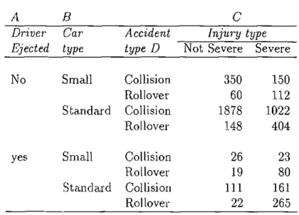
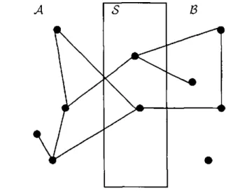
3.4 The global Markov property 75 3.5 Conditional independence graph for collision-rollover data; A is

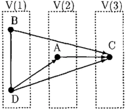
Driver ejected, B is Car type, C is ïnjury and D is Accident type 77 3.6 Chain graph with the dependence chain {A} U {B, C} U {D} . 80 3.7 Chain graph corresponding to graphical chain model for

collision-rollover data, with dependence chain {B}D} U {A} U {C} , , 81

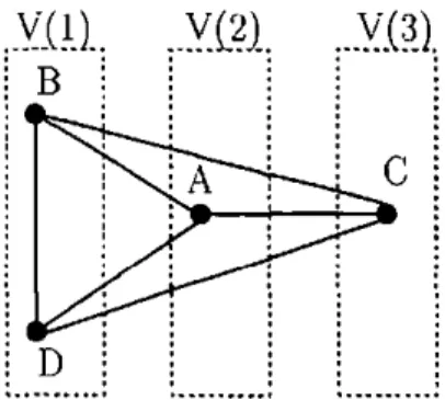
3.8 Moral graph for the chain graph corresponding to graphical chain model for collision-rollover data, with dependence chain

{B,D}U{A}U{C} 82

(13)

LIST OF FIGURES xii 3.9 Moral subgraph of {A,B,D} 83

5.1 The final graphical model for Bedfordshire data with 6 variables 112 5.2 Conditional independence graphs revealing a more detailed as

sociation structure 116 5.3 Graphical model for Bedfordshire data, chosen by Akaike

crite-rion from the minimal accepted models by Edwards-Havranek

model sélection procédure 119 5.4 Graphical chain model for Bedfordshire data with the depen

dence chain { R, £ , 7\ S] U {N} U {A} . . 121 5.5 Graphical chain model for Bedfordshire data with 10 variables 123

5.6 Graphical model for Hampshire data with 6 variables 126 5.7 A graphical non-decornposable model for Hampshire data with

6 variables 127 5.8 Graphical chain model for Bedfordshire + Hampshire data . . 129

5.9 Initial step of building the chain graph for accident data with

pedestrian casualties in Bedfordshire 1.32 5.10 First step of building the chain graph for accident data with

pedestrian casualties in Bedfordshire 133 5.11 Second step of building the chain graph for accident data with

pedestrian casualties in Bedfordshire 134 5-12 T h i r d step of building chain graph for accident data with pedes

(14)

LIST OF FIGURES xiii 5.13 Graphical chain model for Bedfordshire data; accidents with

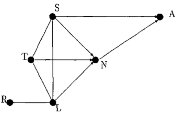
pedestrian casualties only 135 6.1 Graphical model for Bedfordshire data: A is accident severity,

S is speed limit, /V is the number of vehicles involved, T is road

type, L is lighting conditions, R is road surface 144 6.2 Probabilities that an accident on urban and rural roads in Bed

fordshire is fatal 145 6.3 Probabilities that an accident on urban and rural roads in Bed

fordshire is fatal or serious 146 6.4 Graphical chain model for Bedfordshire data with 6 variables . 154

6.5 Graphical model for Hampshire data 158 7.1 Approximate posterior means, calculated from gamma(0.58,0.02),

aga'mst the posterior means of Poisson-log normal model with

p = 2.44 and a2 = 2.45 175

7.2 Approximate posterior means, calculated from gamma(1.17,0.02), against the posterior means of Poisson-log normal model with

/i = 2.44 and a2 = 2.45 176

8.1 Directed graphical model for a mixed Poisson-log normal model 187 5.2 Directed graphical model for a mixed Poisson-gamma model . 192

8.3 Box plots for the models compared 206 5.4 Directed graphical model for Poisson-régression model with gamma

(15)

LIST OF FIGURES xW

8.5 Directed graphical model for Poisson-regression model with mul

tivariate normal random effects 216 5.6 Directed graphical model for a multivariate Poisson-log normal

model 221 9.1 Part of Kent road network 236

9.2 Directed graphical model for the hierarchical Bayesian model

with gamma random effects 242 9.3 Directed graphical model for the hierarchical Bayesian model

with log normal random effects 254 9.4 Sca.tter plots of totals for model (P-ga) 258

9.5 Scatter plots of totals for model (P-logN) 258 9.6 Ranks of means; Poisson-regression with gamma random effects

model 275 9.7 Ordered posterior medians and credible intervals of ranks; model

(P-ga) for first type of accidents 279 9.8 Ordered posterior medians and credible intervals of ranks; model

(P-ga) for second type of accidents 2S0 9.9 Ordered posterior medians and credible intervals of ranks; model

(P-ga) for third type of accidents 280 9.10 Ordered posterior medians and credible intervals of ranks; model

(P-ga) for fourth type of accidents 281 9.11 Ordered posterior medians and credible intervals of ranks; model

(16)

LIST OF FIGURES xv 9.12 Ordered posterior médians and crédible intervais of ranks; model

(P-MNre) for the second type of accidents 282 9-13 Ordered posterior médians and crédible intervais of ranks; model

(P-MNre) for the third type of accidents 282 9.14 Ordered posterior médians and crédible intervais of ranks; model

(P-MNre) for the fourth type of accidents 283 9.15 Comparison of posterior médians of ranks of residual informa

tion; fatal or serious accidents with 1 vehicle, ( P - M N r e ) against

(P-ga) 283 9.16 Comparison of posterior médians of ranks of means; fatal or

serious accidents with 2+ vehicles, ( P - M N r e ) against (P-ga) . 284 9.17 Comparison of posterior médians of ranks of means; slight ac

cidents with 1 vehicle, (P-MNre) against (P-ga) 284 9.18 Comparison of posterior médians of ranks of means; slight ac

cidents with 2+ vehicles, (P-MNre) against (P-ga) 285

C l K S I with 1 vehicle for Model 1 312 C.2 K S I with 1 vehicle for Model 2 312 C.3 K S I with 2+ vehicles for Mode) 1 313 C.4 K S I with 2+ vehicles for Mode! 2 313 C.5 S with 1 vehicle only for Model 1 313 C.6 S with 1 vehicle only for Model 2 313 C.7 S with 2+ vehicles for Model 1 314 C.8 S with 2+ vehicles for Model 2 314

(17)

List of Tables

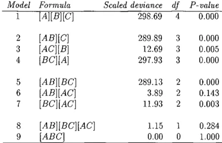
3.1 A 3-way contingency table of road accidents 55 3.2 Models fitted to the collision-rollover data 57 3.3 4-way contingency table of road accidents 58

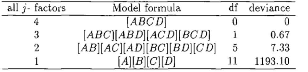
4.1 A l l j-factors models 101 4.2 Tests for Aitkin's model selection procedure 101

4.3 Models selected by Aitkin's procedure 102

4.4 Akaike's criterion values 103 4.5 Marginal and partial association tests 105

4.6 Deviance residuals for the model [ACD][BCD] 107 5.1 3-way marginal contingency table of road accidents 114

5.2 Partitioned deviance tests; the P-values are with 3 decimals . 114 5.3 M i n i m a l accepted models by Edwards-Havranek procedure . . 118

5.4 Bedfordshire 1995 ; a = 0.05 131 5.5 Bedfordshire 1995; a = 0.01 137 6.1 Observed counts for subtables B C D and A C D of collision-rollover

data 147 xvi

(18)

LIST OF TABLES xvii 6.2 Estimâtes for subtables B C D and A C D of collision-rollover data 148

7.1 Means and variances of two prior distributions 176 8.1 Posterior calculations for ail 3 models compared 204 5.2 D1C calculations for ail 3 models compared 205 8.3 Bayesian model sélection for ACD subtable 229 8.4 Bayesian model sélection for BCD subtable 230 5.5 Bayesian forward sélection for Bedfordshire data, ANS subtable 231

8.6 Bayesian backward élimination for Bedfordshire data, ANS

subtable 232 9.1 Total nurnber of accidents for each category of accidents . . . 238

9.2 Posterior means of régression coefficients for mixed

Poisson-gamma model 243 9.3 Proportional réductions in accidents when traffic flow is

re-duced, as resulted from the Poisson-regression model with gamma

random effects 249 9.4 Posterior means of régression coefficients for Poisson-regression

model 251 9.5 Réductions in accident percentages when traffic flow is reduced.

as resulted from the Poisson-regression model without random

effects 252

9.6 Posterior means for mixed Poisson-log normal régression coef

(19)

LIST OF TABLES xviii 9.7 Posterior means of regression coefficients for the Poisson-regression

model with multivariate normal random effects 261 9.S Posterior estimation of parameters of multivariate Poisson-log

normal model 264 9.9 Deviance Information Criterion calculations 26S

9.10 Ranking probabilities for K S I accidents with 1 vehicle 271 9.11 Ranking probabilities for K S I accidents with 2+ vehicles . . . 272

9.12 Ranking probabilities for slight accidents with 1 vehicle . . . . 272 9.13 Ranking probabilities for slight accidents with 2+ vehicles . . 273 B.L Accidents with pedestrian casualties in Bedfordshire, 1995; a =

0.01 309 B.2 Accidents with pedestrian casualties in Bedfordshire and Hamp

shire, 1995; a = 0.05 310 B.3 Accidents with pedestrian casualties in Bedfordshire and Hamp

shire, 1995; a = 0.01 310 B.4 Accidents without pedestrian casualties in Bedfordshire and

Hampshire, 1995; a - 0.05 311 B.5 Accidents without pedestrian casualties in Bedfordshire and

Hampshire, 1995; a = 0.01 311 G . l Estimates for mixed Poissomgamma regression model 336

(20)

Chapter 1

Introduction

1.1 Background

The cost to society of road accidents is very high. According to The Institution of C i v i l Engineers it was estimated in 1996 as being between £14 billion and «£19 billion per annum in the TJK. although it is unmeasurable in terms of human lives (Carruthers, Bulpitt, Gray. Holmes, MacKinven, Moore, Quinn, Zealley and Huxford, 1996). Since road accidents are random events, their occurrence cannot be predicted. Varions factors are thought to contribute to

the réalisation of road accidents. Valuable information can be extracted from large and complex data sets with the help of Statistical methods. Although the exact number of future accidents cannot be calculated, it is possible to predict or estimate this number and to identify some important contributing factors that can be measured and influenced if necessary. What makes ail thèse possible is Statistical modelling.

(21)

CHAPTER l. INTRODUCTION 2

After the second world war the number of accidents increased dramatically but so did the number of vehicles. Governments all over the world were fac ing a serious problem that needed major attention. Statistical methods were soon starting to be applied in this area of research too. However, the major turning point in the advance of scientific methodologies for analysing road accidents has been the development of the theory of generalized linear models (McCullagh and Nelder, 1989). This new class of models is flexible enough to allow modelling of the accident frequencies with a Poisson error. There are sta tistical methods for measuring the safety effect of engineering treatment and for taking into account the regression-to-mean effect (Hauer, 19S0; Hatter, Ng and Lovell, 1989; Hauer, 1997; Wright, Abbess and Jarrett, 1988), and for relating the number of accidents at a site to road network characteristics (Maycock and Hall, 1984; Maher and Summersgill, 1996; Mountain, Fawaz and Jarrett, 1996; Amis, 1996). Comparatively little statistical work has been done on the relationships between accident characteristics such as severity, number of vehicles, pedestrian involvement, time of day and so on. The aim of this research is to contribute to the statistical modelling of large and complex road accident data using and developing appropriate multivariate techniques.

1.1.1 Possible forms of analysis

The statistical investigation of road accident data is a non-randomized study, a kind of observational study in which there is no direct control by the inves tigator. The analyst just observes what is happening, making it very difficult

(22)

CHAPTER 1. INTRODUCTION 3 to establish causal relationships. The nature of this type of data makes im

possible any controlled randomization that would help in designing the study. This îs true for data collected for accident characteristics and summarised in contingency tables and it is also true for data collected for régression-like analyses. For the former case, the analyst takes into account the fact that the accidents already occurred so a rétrospective view is appropriate. In the latter case, the situation is somehow reversed, the task of the analysis being to pre-dict future numbers of accidents using a statistical model that hts the current set of data, again an observational study. A practitioner aims to understand why accidents occur on a road network and what can be done to reduce the number of accidents to a minimum. There are two ways of extracting valuable statistical information from road accident data and thèse perspectives divide the thesis into two parts.

First, various characteristics are recorded for ail accidents which occur in a given period of time. A t a national level this is done in U K each year in a database like S T A T S 19. Then the practitioners might attempt to understand the associations between thèse characteristics that will help them to design better safety policies. Primarily, they are interested in identifying the causes of accidents. However, they cannot analyse each accident individually so they rely on a statistical analysis to identify factors contributing to a large num ber of accidents. Then the local authorities design and implement the safety policies thought to manipula-te the identified factors in such a way to reduce the future number of accidents. It has to be remarked that in statistics the

(23)

CHAPTERL INTRODUCTION 4 word '"causal" is very often avoided in favour of a less powerful term, that

is "association". Nevertheless, studies from other areas of research and some external information may help to identify causes and effects. Maycock (1985) studied 20 variables as road accident factors. VVriting about future possible research he said :

"Fveryone knows that corrélation is not the same thing as cau-sation but the existence of corrélations demand explanations and attempting to obtain explanations would lead into différent sorts of behavioural studies, but studies which were targeted towards explanations of established accident facts,

Moreover, establishing and following up statistical associations in this way could provide fairly direct dues to the design of re médiai measures for those involved in safety législation, éducation and training and the design and administration of driving test standards."

For the analysis of accident characteristics the observational units are the accidents themselves. The variables are the characteristics of the accidents together with other more gênerai variables like road network characteristics, time spécifications and so on. They are analysed in this thesis as categorical, any continuous variables being categorised, and data is summarised in con-tingency tables. This type of data is most of the time recorded by police and it is possible to have miscategorization of some observations due to human error. As highlighted above, for this type of data, one purpose is to nnd a

(24)

CHAPTER 1. INTRODUCTION 5 model which explains how the categorical variables are interrelated. For three

variables A, B and C , if the model suggests that only the pairs A , B and S , C are related, this is formulated statistically as a conditional independence be-tween A and C given the values of B. In common language, knowing the values of variable B may provide some information about possible values of

C, and moreover., Unding out any information about A would be irrelevant for discovering more information about C other than it is already known from B.

For the first kind of data, the approach proposed i n this thesis is based on

graphical modelling and its derivative, graphical chain modelling. W i t h 6 or more road accident characteristics under study, the contingency table can be expected to be sparse. Due to the nature of the data it is a hnite population in a fïxed period of time. This particularity créâtes specific problems that are discussed i n this thesis. O n a real-world example, it is shown that relying on asymptotic inference gives différent results than exact conditional inference and the latter should ahvays be used i n such instances.

The second type of data is analysed by dividing the road network into small units, called sites, and then trying to relate the observed number of accidents to site characteristics, either environmental or socio-economical or géométrie. Depending on the results ot' the Statistical analysis, treatment policies are implemented to reduce the number of accidents. The units of the analysis are the sites and the variables are both discrète (e.g. accident frequeucies) and continuons (e.g. traffic flow).

(25)

CHAPTER!. INTRODUCTION 6 numerical random variables. The units of the statistical investigation are the

sites of the road network. The models proposed in this thesis can be used for prediction of future numbers of accidents, for describing possible correlation structures between accident frequencies of different type and for ranking the sites according to different criteria. Practical applications described here show the usefulness of the joint modelling of multiple accident counts.

Analysing multivariate counts by statistical methods has been very difficult because of the lack of well-defined parametric distributions that can explain complex correlation structures. This problem is solved in this thesis using

hierarchical Poisson multivariate models. The whole methodology used for generalized linear modelling (McCullagh and Nelder, 1989) is incorporated and models with random effects and regression structures are easily and naturally included. However, the complexity of such models makes analytical methods unfeasible. In the modelling process integrals of dimension of hundreds have to be calculated and even numerical methods are not helpful because they are not feasible for dimensions greater than 20. This major difficulty is overcome in this thesis using Markov Chain Monte Carlo ( M C M C ) methods, in particular Gibbs sampling.

The class of hierarchical Bayesian models proposed here is new to ap plied statistical modelling of road accident data because multiple responses are jointly modelled, the models are fully Bayesian in specification and they can be used to answer different questions based on the same statistical M C M C output. Although hierarchical Bayesian models have been developed for

(26)

re-CHAPTER 1. INTRODUCTION 7 peated measurements data in other areas of research, the hierarchical raodels

developed in this thesis are tailored for road accident data. The multiple re-sponses studied in this thesis represent counts of différent type of accidents, so the possible corrélation structure of the responses is not caused by studying the same model over time, like in longitudinal studies. The novel multiplica tive équations describing the models can be used by practitioners to predict changes i n accident type as well as frequency if treatment policies are imple-mented.

It is somehow regretable that the term "hierarchical" has différent mean-ings in the two parts of the thesis. In connection with a log-linear mode! for contingency tables, hierarchical means an imposed rule of model spécification, very important for the interpretability of the models. Regarding a prédictive accident model, hierarchical is again about model spécification but in a totally différent manner. The observed data is combined with a prior distribution for the model parameters; the prior also dépends on some unknown parameters which follow a hyper-prior and the spécification may continue like that on several stages. The hierarchy is ended at some stage where ail the parameters are known.

1.1.2 Graphical représentation

The two directions of research are related by the basic method of represent-ing hiérarchies, which is a graph. In the discussion of the articles given by Wermuth and Lauritzen (1990) and Edwards (1990), A . P . Dawid strongly

(27)

sup-CHAPTER 1. INTRODUCTION 8

C

Figure 1.1: Graphical association model

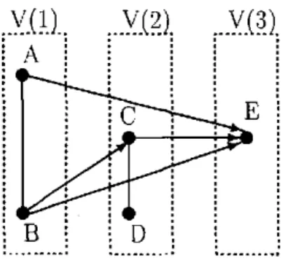
portée! the use of graphs for communicating statistical modelling ideas. In this thesis, two types of graphical models, therefoi'e of graphs, are used. The first type, like the one illustrated in Figure 1.1, has vertices associated with ob-served categorical variables representing accident characteristics. The graph synthesizes the conditional independencies revealed by the graphical model fitting the data. Similar graphs with a mixture of undirected and directed edges will be encountered in the first part of this thesis. Regardless of the nature of the edges, thèse graphs are built using observed variables.

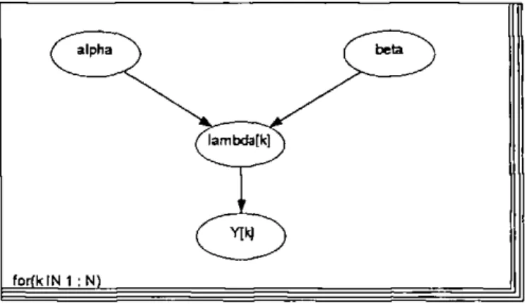
The second type of graphs are used in this thesis again for model spéc ification, more exactly for expressing conditional independencies. There are only directed edges due to the hierarchical structure of the models. T h e dif férence relative to the first type consists in having vertices for observed and unobserved quantities. À simple example is giveu in Figure 1.2. The program W i n B U G S uses such a graphical model for simulation.

In addition, there are some other links between the two main parts of the thesis. T h e analysis of the characteristics of accidents in Bedfordshire

(28)

CHAPTER1. INTRODUCTION 9

( alpha \

/^imbda[kr)

( beta ^ \

forfkIN 1 :N1

Figure 1.2: Directed graphical model for Bayesian model spécification in Win-BUGS

and Hampshire data sets reveals that the accident severity and the number of vehicles involved in the accident are directly related. This suggests that developing separate régression models for thèse two variables may give unreli-able results. The research carried out in the second part of the thesis conhrms this hypothesis and provides a feasible methodological solution. Regarding the model sélection procédures for (hierarchical) graphical models, a new method is proposed i n a Bayesian framework, ernploying similar Markov Chain Monte Carlo ideas as those used for the multiple response variables models. This method provides another link between the two parts of the thesis.

1.1.3 Data sets used

Two separate sources of data were used in this thesis. The first was the S T A T S 19 database for 1995, obtained from U K E S R C Data Archive by the

(29)

Trans-CHAPTER 1. INTRODUCTION 10 port Management Research Centre at Middlesex University. The two subsets

of data extracted from S T A T S 19 and the subset of variables analysed were the author's choice. Some of the variables, like accident severity, were used as recorded in the database but others were recategorised to have a small num ber of levels. For example, the number of vehicles involved and the number of casualties were considered with only three levels (one, two, three or more), road surface conditions with only three (dry, wet-damp, snow-ice-frost-flood). Other temporal variables were also categorised as it will be seen in later chap ters.

The set of data analysed in the second part of the thesis contains the accident frequencies on 156 single-carriageway link sites between 1984 and 1991 in Kent. The data had been provided by Kent County Council to Middlesex Univer sity's Transport Management Research Centre for a previous research project (Mountain, Jarrett and Fawaz, 1995; Mountain, Jarrett and Wright, 1994). The accident counts are known at a disaggregated level; four separate cate gorises were investigated. The disaggregation was made by the author linking the original set of data with the S T A T S 19 database. Covariate information, such as estimated traffic flow, speed limit and link length, was also available and used in the modelling process. Speed limit was considered as a binary vari able having only two levels: urban meaning 40 mph or less and rural meaning 50 mph or 60 mph.

It is well known that not all road accidents are recorded in S T A T S 19 data base (Department of Transport, 1996). The number of unreported accidents

(30)

CHAPTER I. INTRODUCTION 11 is not known and the analysts try to make the best of what is available. In this

thesis the sets of data are used without trying to account for missing records.

1.2 Aims of the thesis

The overall aim of this thesis is to contribute to the development of sound statistical techniques that can be applied to road accident data. The intention is to develop statistical methods which improve the extraction of relevant information contained in the data, information that can be used subsequently by various organisations and traffic engineers to design safety measures. If the wrong sites are selected for treatment due to bad ranking methods, or policy measures are designed to improve irrelevant (from the safety point of view) characteristics of road accidents, the loss is very high in terms of money and human life.

Graphical models and graphical chain models are described as an ex ploratory multivariate technique that can be applied to large sets of road accident data. It is intented to find out which variables, "environmental", "road user", and so on, are associated with variables representing very impor tant accident characteristics, such as accident severity, the number of vehicles involved and the number of casualties.

More specifically, the first part of the thesis has the following objectives 1. To investigate the associations and conditional independencies between

(31)

corre-CHARTER 1. INTRODUCTION 12 sponding to the counties of Bedfordshire and Hampshire, separately and

pooled together.

2. To investigate methods of reducing the analysis of large contingency ta bles to the analysis of a smaller dimensional subtables defined by subsets of variables of particular interest.

3. To investigate various model sélection procédures that can be used in practice for selecting a graphical model; to discuss their advantages and limitations.

4. To investigate the application of graphical chain models when Substan tive research hypothèses are formulated prior to the Statistical modelling process and to identify posible causal implications of such hypothèses. The research carried out in the hrst part of the thesis will use only categor-ical variables, but continuous variables such as trafhc flow are also important in the study of road accidents. The problem is that the theory of graphical models is less well developed for a mixture of discrète and continuous variables. Partly for this reason, the research continues in the second part of the thesis by separating out the individual accidents according to location, in order to relate the accidents to the road network.

In the second part of the thesis the author's aim is to propose a new class of models for différent type of accidents jointly modelled. Models including covariate information as well as models based only on parametric spécification are developed. It is shown how computational problems in developing such

(32)

CHAPTER 1. INTRODUCTION 13 comp lex mo ciels can be solved using M C M C . It is important to relate the

observed number of accidents to environmental characteristics, such as speed lim.it, link length and estimated trafhc flow and this aim will play a major rôle in this thesis in developing the hierarchical models for multiple accident frequencies. The objectives in the second part of the thesis are therefore

1. To develop hierarchical Bayesian models for multiple accident counts. 2. To discuss the problem of ranking the sites according to différent criteria

and considering multiple response variables.

3. To discuss estimation problems for Compound Poisson distributions. This research will beneht authorities in designing new measures for traf hc safety control and new methods for collecting data. A t the same time it will provide some dues and starting points for future studies. The hierar chical Bayesian models will provide a new and deeper Statistical modelling methodology for road accident data.

1.3 Overview of the thesis

This introduction is followed by a Statistical literature review, Chapter 2, where some of the Statistical problems related to the ideas developed in the thesis are defmed and the solutions known so far are illustrated. Although the applications, for which the Statistical techniques are developed, concern road accidents, the same models can be adapted for other count data. The

(33)

CHAPTER 1. INTRODUCTION 14 originality of this thesis consists in taking a multivariate approach for statisti

cal modelling, where ""multivariate" means several responses modelled jointly. Nevertheless the univariate case is also important and is better known in the literature. The role of the Chapter 2 is to review the most up to date statisti cal modelling for the univariate case and to identify potential problems worth discussing in the multivariate setting.

Chapter 3 is concerned with graphical modelling. It provides a motivation for applying graphical modelling to road accident data, describes the graph theory concepts used in the thesis, together with a short account of conditional independence, and gives a detailed description of various Markov properties necessary to develop graphical models and graphical chain models. The theory is almost everywhere accompanied by examples using road accident data.

The inference process is described in Chapter 4. The starting point of dis cussion is the class of log-linear models, a particular case of generalized linear models. When the researcher is interested in identifying conditional inde pendence relationships between the variables (or between groups of variables) under study, graphical models are proposed as one of the best solutions. The theoretical framework and the most important results are described. More over, since it is known that any log-linear model can be nested into a graphical model, it seems to be always useful to find out a graphical model fitting the data well and simply enough to assist interpretation. Various model selection procedures for log-linear models and graphical, models are reviewed and exem plified. The theoretical aspects of graphical chain models are also developed.

(34)

CHAPTER 1. INTRODUCTION 15 The data subsequently analysed in Chapter 5 are aubsets of data extracted

from the national road accident database for Great Britain. S T A T S 19. It is expected that the contingency table summarising such data will be sparse. This particular aspect makes the contingency tables more difficult to analyse. The classical tests based on asymptotic methods are not reliable so exact conditional tests, using Monte Carlo methods to overcome the computational difficulties, are described in the context of graphical models. Graphical mod-els and graphical chain modmod-els for very large sets of data are proposed and important conditional independencies between road accident characteristics are identified. A comparison of asymptotic and exact conditional methods is investigated in relation to graphical chain modelhng, for a large subset of data regarding accidents with pedestrian casualties in Bedfordshire in 1995.

Methods of reducing the dimensionality of the analysis are extremely use-ful. Collapsibility is a concept developed in the context of log-linear modelling that proves extremely belpful in reducing the amount of work necessary to ex tract reliable information from data. This is done in an applied manner in Chapter 6.

Probably the most theoretical chapter of this thesis is Chapter 7 where esti mation problems for Compound Poisson distributions are studied. Two major cases, the Poisson-gamma and Poisson-log normal distributions, are discussed in greater detail. This chapter lias a special importance since many practition-ers seem not to be aware of the difficulties presented by thèse two Compound distributions and Compound Poisson distributions in gênerai. Chapter 7

(35)

con-CHAPTER 1. INTRODUCTION 16 tinues the discussion started in Chapter 2 about empirical Bayesian modelling

but goes beyond that and opens the door to more complex and realistic models. Chapter 8 is dedicated to hierarchical Bayesian models for counts. Bayesian methods combining hierarchical models and regression techniques are devel oped to extract information from a set of road accident data. In the first section the general methodology is explained in the context of univariate mod els, thus making a straightforward connection with the second chapter of the thesis. M C M C methods are used to solve computational problems related to hierarchical models and are illustrated using two standard models. In the sec ond part of Chapter 8 several complex hierarchical models are developed. A t the same time, an attempt is made to model multiple response count mod els, based solely on the observed frequencies, using distributions such as the multivariate log-normal distribution, hierarchically specified.

A new Bayesian model selection procedure is proposed for log-linear models for contingency tables. The computational side of the new method is solved again by applying M C M C techniques and this is the main reason why this section is included in this chapter.

Given the applied character of this thesis, there is a companion Chapter 9 to Chapter S in which a complex set of accident data is investigated at a mul tiple response level. The set of data concerns accidents on 156 links in Kent between 1984 and 1991. The models analysed are fully Bayesian and range from simple log-linear regression models to mixed Poisson regression models with random effects. First, it is shown how to select a small subset of

(36)

represen-CHAPTER 1. INTRODUCTION 17 tative models (3 models are identifiée!), and then, thèse rnodels are examined

in greater detail. The sites can be ranked according to différent criteria using a single M C M C output, and the results are described and discussed towards the end of the chapter.

The last chapter summarises the conclusions of this thesis, from both theo-retical and applied points of vïew. It also contains a section proposing further research that would follow quite naturally from the results of this thesis.

(37)

Chapter 2

Statistical modelling of road

accident data

2.1 Introduction

The purpose of this chapter is to présent the framework of the thesis in terms of the assurnptions made and the problems that will be tackled, and also to review critically the contingent literature to thèse problems.

Road accidents are among the more visible conséquences of an enormous number of failures in the daily volume of interaction between the people who use the road networks and the environment in which thev travel. A n accident that is predictable is a contradiction in terms. fn other words, when we are talking about an individual accident, no matter how much knowledge we have about the possible generating mechanisms. we are unable to predict exactly where, when and to whom the next individual accident will occur. The best

(38)

CHAPTER 2. STATISTICAL MODELLING OF ROAD ACCIDENT DATA 19 that can be done is to predict their approximate number. This is simply because, although an individual accident is impossible to predict, the total number of accidents of some kind may behave with an almost constant overall frequency in the long run.

As defined in Hauer et al. (19S9) and Hauer (1997) safety is the property of some specific entity, most commonly a site of the road network. The prop erty of safety (or more exactly the non-safety) for a site is quantified as the number of accidents expected to occur per unit of time and their adverse con sequences. The important term is "expected" which makes a straightforward connection with the statistical approach. If all conditions that affect safety (traffic, weather, and so on) are frozen, expected means the "average" in the long run.

One aim of collecting and investigating road accident data is to identify significant clusters of accidents having common causal factors and to asses the expected numbers of road accidents. The list of problems includes the evaluation of safety treatments, the ranking and identification of hazardous locations, predicting the numbers of futures accidents and investigating the associations between characteristics of road accidents. The statistical mod els proposed for solving these problems can be divided into three categories: models for accident frequencies, models for type of accidents and models for both accident frequencies and type of accidents. The first category has been well investigated at univariate level and it is reviewed next.

(39)

CHAPTER 2, STATISTICAL MODELLIN G OF ROAD ACCIDENT DATA 20

2.2 Models for accident frequencies

The following methodological Framework is followed for studying accidents counts on a road network over a fixed period of time. T h e network is first divided irito units. usually cailed sites, like junctions or Stretches of the road. The Statistical unit is the road network element and the response variables are accident counts.

2.2.1 The pure Poisson Model

The main probability distribution used in modelling accident data is the Pois son distribution. Accidents occur in time. Consider a fixed site for which ac cidents are recorded i n a hxed period of time T. Partitioning the time period into n intervais of duration T/n, let YUii be the number of accidents recorded

in the i-th time interval. let Pnj — Pr(yn ] I- — 1) and let en,i ~ Pr(YnA > 2).

The following assumptions are made

1. T h e random variables Ynti, (i = 1 , 2 , . . . . n) are independent over i

2- E S ï - P » , ; -> A € (0,co) as n -» co, 3. maxi<i<n Pnj —» 0 as n —> oo,

4- en,i -* 0 as n -> oo.

Then it is shown in Durrett (1991, Theorem 6.1) that

(40)

CHAPTER 2. STATISTICAL MODELLING OF ROAD ACCIDENT DATA 21 vvhere d means that the convergence is in distribution. This justifies using the Poisson distribution for modeliing road accidents. This dérivation is concep-tually différent from the one based on a homogeneous Poisson process and the Poisson distribution that characterizes it. The assumption of a homogeneous Poisson process is not valid for road accidents since it is natural to expect great variation of accidents by time patterns.

The Poisson distribution is defined mathematically and whether a séries of events is i n agreement with it is an empirical fact. Dénote by Yk the number of accidents at site k during an observed time period Tk- The first assumption

made in modeliing accident frequencies (Nicholson, 1985) is that

Yk I mk ' ~ Pois(mA = Af cT*)

where h = 1,2, ....N and A;, is the mean accident frequency per unit time at site k. The expected number of accidents, mjt, can then be linked with a covariate vector Xk = {Xk\, Xk2t • - • > X^q)'. representing for instance traffic flows and the géométrie characteristics of the site. The connection is made via a multiplicative équation which can be transformée! into a linear équation on the logarithmic scale. The unknown coefficients are estimated by fitting the model to data and thèse will be used for statistical inference. The fitting process, under this generalized linear statistical modeliing framework. can be done in G L I M or G E N S T A T , where maximum likelihood estimâtes are obtained using an itérative weighted least squared ( W L S ) procédure. The

(41)

CHAPTER 2. STATISTICAL MODELLING OF ROAD ACCIDENT DATA 22 most common goodness-of-fit measures used are

k=N G2 X2

X ^ L l o g ^ )

(yk -mky - (yk - rnk) k=N f „ ^2 (2.1) (2.2)

where yk(k = 1 , 2 , . . . . iV) are the observed number of accidents and are the estimated means under the fitted model. The above notation for the Poisson model will be used without any index accounting for différent sites when the theoretical model in itself is the same for each site and the model is self-explanatory.

Regarding the accident frequencies observed on a fixed number of sites, there are two broad types of statistical investigations:

1. before-after studies; and

2. régression models regarding the prédiction of future number of accidents.

2.2.2 Before-after studies

A safety treatment of a site of a road network aims to reduce the number of accidents at that site. The usual way of assessing the effectiveness of a safety treatment is to compare tire accident frequency before the treatment has been implemented with that after treatment.

A réduction in accidents at the treated sites does not necessarily imply that the treatment has been successful. Three reasons may be responsible for this.

(42)

CR AFTER 2. STATISTICAL MODELLING OF R.OAD ACCIDENT DATA 23 • The number of accidents at a site may change in a random manner,

increasing or decreasing. whether or not there has been any change at the site. Statistical methods are necessarv to consider this random variation. • The mean number of accidents may decrease without any connection

vvith the treatment. In order to study these systematic factors it is important to compare treated sites with a control group of untreated sites. The confounding effects, such as time, can be overcome by selecting a control group of sites and observe the number of accidents at these sites over the same period as the treated sites. This design is called the before-after study and it uses a 2 x 2 contingency table

Control Treatment Before nn ni2

After «21 « 2 2

defined by the time dichotomy, before-after, and the control-treatment dichotomy.

• The thircL problem. is the régression-lo-mean effect, which means that for the many sites with a "low"'"' accident frequency before treatment there will be a slight rise after treatment, for the few sites with a "high" frequency a greater fall; while for all sites together, no change, (Hauer,

1980).

The first two problems can be solved by standard methods (Hauer, 1986; Hauer, 1980; Hauer, 1997). In terms of improvement due to the Statistical

(43)

CHAPTER 2. STATISTICAL MODELLING OF ROAD ACCIDENT DATA 24 analysis, the third problem is viewed as one of the most important. The regression-to-mean bias inadvertently results from the fact that only locations with a large number of accidents are generally selected for treatment, which may lead to biased conclusions. The standard solution to this problem is to use empirical Bayes ( E B ) models as developed in Abbess, Jarrett and Wright (1981), Jarrett, Abbess and Wright (1982), Brude and Larsson (1988), Mor ris, Christiansen and Pendleton (1991). Hauer (1997) is a general reference explaining empirical Bayes methods for practitioners.

The empirical Bayes ( E B ) method for estimation provides a general frame work where different distributions can be studied in order to improve the qual ity of the estimators. The compound model

Yk | ™>k l~ Pois(m/.) (2.3)

mk ~ G'(-) ke { 1 , 2 , . . . .JV}

lead to estimates of the individual parameters using information from all sites under study. In studies using E B methods the variation of rajt from site to site is regarded as purely random. Then the Yk are marginally independent.

If the unknown distribution G(-) has probability density g then the marginal density is

(44)

CHAPTER 2. STATISTICA L MODELLING OF ROAD A CCIDENT DATA 25 and the posterior density of mk is

Poi$(yk\Tnk)g(mk)

Pc(Vk) (2.4)

If g is known. meaning that its parameters are given and do not have to be estimated. then the model is called fully Bayesian; if the parameters of g have to be estimated from data then this approach is called an empirical Bayes (EB) method.

One of the first important empirical Bayes ideas for modelling counts was advocated by Robbins (1955) in a nonparametric form. For the componnd Poisson-G model described in (2.3), suppose that G is totally unknown. Under squared error loss ( S E L ) , the Bayes estimator is the posterior mean

The M L E of m is y so raB is biased. However, m is preferred because of

lower M S E . When G is known, the estimation is straightforward. For the case when G is unknown Robbins (1955) suggested to estimate pc[y) by the number of values Y in the sarnple Y\, V2, - - •, YN that are equal with Y, so

m B E(m\y) (y + l ) p g ( y + l ) Pc(y) (2.5) (2.6) mu = {y + l)

(45)

CHAPTER 2. STATISTICAL MODELLIN G OF ROAD ACCIDENT DATA 26 information from other sites as well. Although this procédure has some good asymptotic properties, it was shown that, even when the sample size is large, this method does not perform very well and a parametric approach is more suitable (Carlin and Louis, 1996).

The prior distribution g (m) is usually assumed to be of gamma form, because the gamma distribution is the conjugate distribution for the Poisson distribution (George. Makov and Smith, 1993). Thus

/ \ a a /rt -%

m ~ gamma(a, o) = gamma 7 ; — • (2-0 L6' 62

where gam.ma(x | a, b) = J ^x a-le -x b and the second parameterisation is i n

terms of the mean | and variance ^ . Then it follows from the Bayes formula in équation (2.4) that the posterior distribution of m is

p(

m

1 y) = T [ ^ y

m

°

+

" "

v ( m , m ( 2

'

8 )

The marginal distribution of Y is then

which is a negative binomial distribution NB(-j-^, a). As described by Morris in discussionof Haueret al. (1989), thewhole parametricmodellingmethodology for accident counts can be expressed in terms of a descriptive model and an

(46)

CHARTER 2. STATISTICAL MODELLING OF ROAD ACCIDENT DATA 27 distribution of the unobserved parameters. T h e descriptive model is given by

• observed data

Y ^ Pois(m) (2.10)

• unobserved parameters

m \ a, 6 ~ gamma(a, 6) = gamma a a

[V p

(2.11)

The inferential model is then • observed data Y ~ N B [ p = 1 + 6' (2.12) • unobserved parameters m | y ~ gamma(a + y, b + 1) = gamma a

+

y a

+

y . 6 + l ' ( è + l )2J (2.13)

The Bayes estimate of m for the subpopulation of those sites at which y accidents occurred is

E ( m | y) = a + y

6 + 1 (2.14)

(47)

CHAPTER 2. STATISTICAL MODELLING OF ROAD ACCIDENT DATA 28 définition is the expected percentage change in the number of accidents

R = E ( m \ y)-y x 100

n + yf_ y

b+ly x 100.

In order to calculate the régression effect R the values of pararaeters a and b need to be estimated. The values of thèse parameters can be estimated by htting the négative binornial distribution, équation (2.9). to the observed data. This can be doue in G L I M using macros or more directly in G E N S T A T . Some examples of such analyses are in Persaud (1991), .larrett et al. (1982), Hauer (1997).

The Bayes estimate mB is a convex combination of the overall expected

accident frequency /i and the observed frequency y

mB — E ( m I y) = a + y m = 6 + 1 ap + (1 - ct)y (2.15) (2.16)

where a = 7^7, ju = E ( m | a,6) = |. It is worth pointing out that a dépends on var(m) in the population of sites.

Another way of modelling the effect of a safety measure implemented at a site is to define a coefficient 0 such that

(48)

CHA PTER 2. STATISTICAL MODELLING OFROAD ACCIDENT DATA 29 where the two m values represent the expected number of accidents, before and after the implementation. If the remédiai treatment has no effect then

0 = 1. ï h e différence from this value can be interpreted as an increase or decrease by the same percentage in the expected number of accidents. The value of 0 is estimated as shown in Kulmala (1994).

There are other methods for dealing with the regression-to-mean effect, though they are more difhcult to apply i n practice (Wright et al., 1988). However, only the E B methods are important for the development of the models considered in the second part of the thesis. Wright et al. (1988) describe four main problems about the assumptions made for ail methods that need to be carefully considered.

1. The first problem is about the définition of the term "site". For treated sites this is done by local authorities and this may influence the estimate of the true accident rate for that site in future years. However. for the régression models considered i n the next subsection and later chapters, the road network is usually divided into nodes (jmictions) and links. 2. The second problem is about defining the population. For a given site,

do " a i l " the sites in the study area dehne the population or only "those" with similar physical characteristics as the treated site? The régression models allow the parameters of the gamma distribution to dépend on site characteristics, so the 'population' consists of ail sites with the same characteristics.

(49)

CHAPTER 2. STATISTICAL MODELLING OF ROAD ACCIDENT DATA 30 3. The third problem concerns the "gamma assumption". Following Abbess

et al. (1981). this means that the distribution of the true mean accident rates is gamma. This is very convenient from the mathematical point of view but it is a strong assumption. It would be very interesting to know how sensitive the results are to this assumption and whether other distributions such as log normal give satisfactory solutions. Some new approaches are described in this thesis in Chapters 7 and 9.

4. The remedial sites are chosen for treatment because they have a large number of accidents which appear to have causal factors in common. The fourth problem is whether the regression-to-mean effect can be studied in terms of the overall accident frequency at each site. A simultane ous analysis of accident frequencies of various type would certainly be more beneficial. Statistical models for doing this kind of analysis after disaggregation are developed in Chapters 8 and 9.

2.2.3 Regression models for accident frequencies

Very often, a better prediction of future number of accidents is posssible when the covariate information available is linked to the observed number of acci dents. This will help in establishing a straightforward method for prediction. Linear regression models using a normal distribution for the error term are not appropriate. Generalized linear modelling gives better modelling flexi bility and the predictive accident models developed in the last two decades are included in this general framework. This allows retention of the

(50)

Pois-CHAPTER 2. STATISTICAL MODELLING OF ROAD ACCIDENT DATA 31 son assumption. Therefore, Poisson log-linear modelling is often used for the régression models for road accident data.

A generalized linear model, McCullagh and Neider (1989), is specîfied by

Y ~ f{9,è) (2.17)

E(Y') = m (2.18)

h(m) = X'ß. (2.19)

In this, À' is a vector of explanatory variables. The relationship between the mean m and the linear predictor X'ß is modelled by the so called link function

h. This is possible as long as there is a function h* such that 0 = h*(Xfß).

When the error distribution /(0, <j>) is Poisson with mean m the canonical link

0 = log (m) = X'ß leads to the standard log-linear Poisson-régression model.

Regression models

In the literature there are studied several classes of régression models. A Poisson cla-ss of models (Miaou and L u m . 1993) assumes that

Y - Pois(m) (2.20)

m = E(Y) - v[exp(X'ß)] (2.21) where v is an exposure factor. like time for instance. The rate function is

(51)

CHAPTER 2. STATISTICAL MODELLING OFROAD ACCIDENT DATA 32 régression model, Maycock and Hall (1984), is described by

Y ~ Pois(m)

m = E ( T ) =iA[exp(X'ß)]

where the unknovvri constant ß0 rieeds to be estimated. If u is a good exposure

measure then the estimated ß0 should be close to 1.

As pointed out in Miaou and Lum (1993), the Poisson distribution is very useful not only because tests and confidence sets for the estimated régression coefficients can be calculated, but probabilistic statements can be made about

Y. This is an important point in favour of using the Poisson distribution, which is discrète. Thcre is no need to look for some other continuous distributions, like the normal that is still used, quite inappropriately, i n some investigations, for example Amis (1996).

For prédictive accident moclels traffic flow plays a major role, and should also be considered in before-after studies. Changes in trafFic flows influence changes i n accident counts between the "before" and "after" periods, and this should be accounted for before making any claims about the effectiveness of any treatment. Traffic flow is also important for estimating the expected accident numbers, and is usually included amongst the explanatory variables À'. Quite often accident rates like accidents/vehicle kilometer are used to account for changes in traffic flow as a measure of exposure. This would be correct if the expected accident frequencies like accidents/year were directly

(52)

CHAPTER2. STATISTÏCAL MODELLING OF ROAD ACCIDENT DATA 33 proportion al to traffic flow. This common belief is seldom true; the coefficient of flow is significantly différent from 1.

A further problein is that the exact values for traffic flows are not known and they are replaced by estimâtes. This may cause further problems if there are random errors in thèse estimâtes. If Q is the traffic flow count and z is the true annual average daily traffic ( A A D T ) flow. they can be modelled at the same time using the following model

Y ~ Pois(m = AT) (2.22)

Q ~ Pois(^) (2.23)

m = 71e x p [ X/^ + l o g ( z )7] . (2.24)

A n itérative procédure described in Maher and Summersgill (1996), can be used to calculate the estimâtes of the unknown parameters (/?,7).

T h e Overdispersion problem

One limitation of the Poisson-régression modelling. well documented in the literature, is that the error variance bas to be equal to the mean Ë ( K ) in équation (2.18), see Cox (1983) and Dean and Lawless (1989). However, in practice count data very often shows overdispersion: the error variance is greater than the mean. Ignoring this phenomenon can be very troublesome. Although the maximum likelihood estimators of the régression coefficients are still consistent, the variances of the estimated coefficients tend to be

(53)

underes-CHAPTER 2. STATISTICAL MODELLING OF ROAD ACCIDENT DATA 34 timated, which means that the significance levels of the estimated coefficients can be misleading. The phenomenon of overdispersion is well-known in many areas of statistics. There are several methods to overcome this difficulty but there is much research under progress searching for better solutions. Some pos sible reasons for overdispersion in prédictive accident models are commented in Maher and Summersgill (1996).

Overdispersion occurs quite often in modelling count data under a Poisson assumption. so the first attempts to solve this problem were based on making more complex distributional assumptions. One solution proposed by Wed-derbnrn (1974) to correct for overdispersion is a quasi-Poisson model (QP)-The différence from the classical Poisson model is that var(F) = r m , with the parameter r accounting for overdispersion. This parameter can. then be estimated by any of G2/{N - p), A"2/(iV - p), or G2/ E ( G2) , where N is the

number of observations and /; is the number of parameters estimated. Sim ulation studies (Maher and Summersgill, 1996) have shown that the second performs better. For the estimâtes of the régression parameters there is no différence compared to the pure Poisson model, but their standard errors are inflated by a factor of %Jr. The asymptotic i-statistic for the coefficient of régression can be improved (Agresti, 1990) by multiplying the value for the initial i-statistic, obtained from the Poisson régression model, by T ~ 2 . One may obtain the correct adjusted asymptotic standard errors by multiplying the values given by traditional generalized linear modelling software by the scaling factor y/r = JX^KN — p). The inference is then performed in the

(54)

CH AFTER 2. STATISTICAL MO DELLING OF ROAD ACCIDENT DATA 35 classical manner using thèse adjusted asymptotic standard errors. It can be immediately seen that, when r > 1. Le. there is overdispersion, the confidence intervais obtainecl after adjusting are larger than the unadjusted confidence intervais. Thus. the inferential process is improved by using the correct as ymptotic standard errors.

A n alternative is to use another discrète distribution instead of the Poisson distribution. Following a Bayesian approach as described above, it seems that the negative binomial distribution (NB) is more suitable, as it allows the variance to be greater than the mean. A third more gênerai solution is to use a more gênerai family of negative binomial distributions for which ( Q P ) and (NB) models are just two special cases (Cameron and Trivedi, 1986). This gênerai model is given by the following assumptions

Yk ~ ?o\s{\kTk), for ail A

\k ~ gamma(r?.6) = gamma

(2.25) (2.26) (2.27)

where a is a constant factor and the overall mean f_i is estimated from the data. From the model spécification it follows that

p(Yk | ß,b) = N B E(Yk\fL,b) lTk ,b + Tk var(V* 1/1,6) = E(Yk \ ^ b)b-±J± = //f, ( l + ^ ) (2.28) (2.29) (2.30)

(55)

CHAFTER 2. STATISTICAL MODELLING OFROAD ACCIDENT DATA 36 Using équation (2.27) it follovvs that b = afiJ~l, and this means that

u2~jT2

var(yf c | ii, b) = fxTk + h- k

-a

as mentioned in Mäher and Summersgill (1996). Thus, j = 0 implies that

?/ = a and this is the ciassical N B model used. If j = 1 it follovvs that n = a/j, so the shape of the gamma distribution is not constant and it dépends on its mean. In this case

var(Vf c|/i,6) = //r ^ l + ^

and if Tk = T then this model becomes a (QP) model with r = 1 + ~.

This methodology can be extended to incorporate covariate information; the parameter \i is then a function of the covariate vector X. In this family of models, for the T R L studies, like the T R L 4-arm roundabout study (Maycock

and Hall. 1984), it seems that the (NB) model is more adéquate than the (QP) model.

2.3 Selecting sites for treatment

2.3.1 Introduction

The main job of traffic safety engineers is to correct hazardous sites. First, they have to identify the risky locations, then to détermine remedial schemes and in the end to implement the best feasible treatment. Choosing the wrong sites is damaging in two ways: firstly, some hazardous sites may be left

(56)

un-CHAPTER 2. STATISTICAL MODELLING OF ROAD ACCIDENT DATA 37 treated and secondly, large amounts of public money are was ted. Ideally, sites should be ranked by the values of their true means m. These are unknown, but because of random variation, observed numbers of accidents are not en-tirely reliable. Statistical modelling is often used to improve the methodology. Similar problem s are addressed in mediane (Morris and Christiansen, 1996), where profiling hospitals lias become very important in récent years, and in éducation (Laird and Louis, 1989), where ranking schools based on pupil per formance data is required for public information and for implementation of better éducation policies.

Ranking and sélection are related to either a "relative" given set of Statisti cal units, in our case sites, and then the units are just compared to each other, or to an "absolute" standard like a given threshold and the purpose is then to identify those units that exceed the threshold. Ranking can be successfully used to indicate good or bad performance. Ranks should contain Statistical information that avoid misrepresentation of the précision of estimation. If régression methods can be used to explain the whole between-sites variation there is no basis for ranking.

Generally, sites are ranked according to some safety measure such as acci dent count or rate. Higle and Witkowski (1988) were the first to propose (EB) methods for ranking locations. The (EB) methods were used to give greater weight to those sites having greater exposure. They were not used because of sélection bias, which is not of concern here. The site estimâtes are différent in their reliability. For example, if a large number of accidents y\ is observed

(57)

CHAPTER 2. STATISTICAL MODELLING OF ROAD ACCIDENT DATA 38 at a site with a high exposure, then there is more confidence that yi is close to its true mean value than for a large number yi accidents observed at a site with low exposure.

Ranking the sites by their empirical accident frequency, without consid ering the uncertainty of each estimate, may not correctly identify the worst locations. Nothing can be said about the probability that the worst sites have been selected or about the extent to which the selected sites are really haz ardous compared with the non-selected ones. Bayesian and empirical Bayes methods have been used to overcome some of these difficulties, see Hauer (1980), Higle and Witkowski (1988), Davies (19