Semi-supervised Learning in Graphs
Alberto Bertoni, Marco Frasca, and Giorgio Valentini
DSI, Dipartimento di Scienze dell’ Informazione, Universit`a degli Studi di Milano, Via Comelico 39, 20135 Milano, Italia {bertoni,frasca,valentini}@dsi.unimi.it
Abstract. The semi-supervised problem of learning node labels in graphs consists, given a partial graph labeling, in inferring the unknown labels of the unlabeled vertices. Several machine learning algorithms have been proposed for solving this problem, including Hopfield networks and label propagation methods; however, some issues have been only par-tially considered, e.g. the preservation of the prior knowledge and the unbalance between positive and negative labels. To address these items, we propose a Hopfield-based cost sensitive neural network algorithm (COSNet). The method factorizes the solution of the problem in two parts: 1) the subnetwork composed by the labelled vertices is consid-ered, and the network parameters are estimated through a supervised algorithm; 2) the estimated parameters are extended to the subnetwork composed of the unlabeled vertices, and the attractor reached by the dy-namics of this subnetwork allows to predict the labeling of the unlabeled vertices. The proposed method embeds in the neural algorithm the “a priori” knowledge coded in the labelled part of the graph, and separates node labels and neuron states, allowing to differentially weight positive and negative node labels. Moreover,COSNetintroduces an efficient cost-sensitive strategy which allows to learn the near-optimal parameters of the network in order to take into account the unbalance between pos-itive and negative node labels. Finally, the dynamics of the network is restricted to its unlabeled part, preserving the minimization of the over-all objective function and significantly reducing the time complexity of the learning algorithm. COSNet has been applied to the genome-wide prediction of gene function in a model organism. The results, compared with those obtained by other semi-supervised label propagation algo-rithms and supervised machine learning methods, show the effectiveness of the proposed approach.
1
Introduction
The growing interest of the scientific community in methods and algorithms for learning network-structured data is motivated by emerging applications in sev-eral domains, ranging from social to economic and biological sciences [1, 2]. In
D. Gunopulos et al. (Eds.): ECML PKDD 2011, Part I, LNAI 6911, pp. 219–234, 2011. c
this context a fundamental problem is represented by the supervised or semi-supervised node classification, i.e. predicting node labels by exploiting the re-lationships between labeled and unlabeled nodes of the network. Instances are connected via a set of links, and a learner relies on the assumption that linked entities tend to be assigned to the same class label. For example, in protein-protein interaction networks genetic or physical interactions coded in the links of the network bear witness to common biological processes or molecular func-tion activities between linked proteins [3]; in social networks, people that are friends often share similar characteristics or commons interests [4]; in document classification, texts that are linked through common citations often share similar topics [5].
Several approaches have been proposed in literature to classify networked data. They usually represent data through an undirected graph G = (V, W), where nodes v ∈ V correspond to instances to be classified, and W defines the weights of the edges according to the “strength” or the evidence of the relationships between pairs of nodes.
The first and simplest algorithms proposed were based on “guilt-by-association” methods, by which unlabeled nodes are set according to the majority or the weighted majority of the labels in their neighborhoods [6, 7]. By extending this approach, nodes can “propagate” their labels to their neighbors iteratively by re-peating this “label propagation” process until convergence [8, 9]. In this context Markov Random Walks can be applied to tune the amount of propagation we allow in the graph, by setting the length of the walk across the graph [10, 11]. Other related methods are based on smoothness considerations that yields to graph regularization [12, 13], or exploit the properties of the graph Laplacian associated to the weight matrix of the network [14]. Algorithms based on the evaluation of the functional flow in graphs [3, 15], on Markov [16] and Gaussian Random Fields [17, 18] have been applied to the prediction of gene functions in biological networks. Hopfield networks [19] shares common elements with label propagation algorithms. Indeed labels are iteratively propagated across the neighbors of each node and a quadratic cost function related to the con-sistency of the labeling of the nodes w.r.t. the network topology is minimized by the network dynamics. From this standpoint Hopfield networks and most of the proposed graph-based algorithms for the prediction of node labels can be cast into a recently proposed common framework where a quadratic cost objective function is minimized [20]. Nevertheless, there are some issues that have been only partially considered in classifying networked data. Many of the graph-based approaches do not preserve prior information coded in nodes label-ing, and are unable to effectively predict node labels when data are unbalanced, e.g. when negative nodes significantly outnumber positives. This issue is par-ticularly relevant when label propagation algorithms are applied to predict the functions of genes, since positive annotations are usually much less than negative ones [18]. Despite some cost-sensitive variants of Gaussian Random fields have been proposed, they are based on simple class rescaling so that their respective weights over unlabeled examples match the prior class distribution estimated
from labeled examples [8, 18]. Finally, many approaches based on neural net-works do not distinguish between the node labels and the values of the neuron states [21], thus resulting in a lower predictive capability of the network.
To address these issues, we propose a cost-sensitive neural algorithm (COSNet), based on Hopfield networks, whose main characteristics are the following:
1. Available a priori information is embedded in the neural network and pre-served by the network dynamics.
2. Labels and neuron states are conceptually separated. In this way a class of Hopfield networks is introduced, having as parameters the values of neuron states and the neuron thresholds.
3. The parameters of the network are learned from the data through an efficient supervised algorithm, in order to take into account the unbalance between positive and negative node labels.
4. The dynamics of the network is restricted to its unlabeled part, preserving the minimization of the overall objective function and significantly reducing the time complexity of the learning algorithm.
In sect. 2 the classification of nodes in networked data is formalized as a semi-supervised learning problem. Hopfield networks and the main issues related to this type of recurrent neural network are discussed in Sect. 3 and 4. The problem of the restriction of network dynamics to a subset of nodes is analyzed in Sect 5, while the proposed neural network algorithm, COSNet (COst Sensitive neural Network), is discussed in Sect. 6. In the same section we show that COSNet
covers the main Hopfield networks learning issues, and in particular a statistical analysis highlights that the network parameters selected by COSNet lead to significantly lower values of the the energy function w.r.t. the non cost-sensitive version of the Hopfield network. In Section 7, to test the proposed algorithm on a classical unbalanced semi-supervised classification problem, we applied COS-Net to the genome-wide prediction of gene functions in a model organism, by considering about 200 different functional classes of the FunCat taxonomy [22], and five different types of biomolecular data. The conclusions end the paper.
2
Semi-supervised Learning in Graphs
Consider a weighted graphG= (V, W), whereV ={1, . . . , n} is the vertex set andW = (wij) is the symmetric weight matrix: the weightwij ∈Rdenotes a similarity index of nodei with respect to nodej. The vertices inV are labeled with{+,−}, leading to the subsetsPandNof positive and negative vertices, but the labeling is known only for a subsetS⊂V, while is unknown forU =V \S. Let be S+ =S∩P and S− = S∩N: we can refer to S+, S− and W as the
“prior information”.
The semi-supervised classification problem consists in finding a bipartition (U+, U−) of nodes inU relying on the prior information. Nodes inU+ are then
considered candidates for the classP∩U.
A reasonable measure of the “correctness” in approximatingP∩U byU+and
defined as follows: by calling false positives the vertices F P = U+∩N, false negatives F N = U−∩P and true positives T P = U+ ∩P, the F
score is the harmonic mean between precision and recall, where precision = |T P|T P|+|F P|| ,
recall= |T P|T P|+|F N|| . Note that 0Fscore1 andFscore= 1 iffU+=P∩U.
3
Hopfield Networks
By slightly generalizing the classical definition of discrete Hopfield networks (DHNs) [19], a Hopfield networkH with neurons V ={1,2, . . . , n} can be de-scribed by a tripleH = < W, γ, α >, where:
- W is an×nsymmetric matrix in whichwij ∈Ris the connection strength between neuronsiandj, withwii= 0 for eachi
- γ= (γ1, γ2, . . . , γn)∈Rn is a vector of activation thresholds
- αis a real number in [0,π2] that determines the two different values{sinα,
−cosα} for neuron states.
At each discrete timeteach neuronihas a valuexi(t)∈ {sinα,−cosα} accord-ing to the followaccord-ing dynamics:
1. At time 0 an initial valuexi(0) =ai is given for each neuroni
2. At timet+ 1 each neuron is updated asynchronously in a random order by the following activation rule
xi(t+ 1) = ⎧ ⎪ ⎪ ⎨ ⎪ ⎪ ⎩ sinα if i− 1 j=1 wijxj(t+ 1) + n k=i+1 wikxk(t)−γi>0 −cosα if i− 1 j=1 wijxj(t+ 1) + n k=i+1 wikxk(t)−γi≤0 (1)
The state of the network at timet is the vectorx(t) = (x1(t), x2(t), . . . , xn(t)).
The main feature of a Hopfield network is the existence of a quadratic state function, i.e. theenergy function:
E(x) =−1 2x
TW x+xTγ (2)
This is a non increasing function w.r.t. the evolution of the network according to the activation rules (1), i.e.
E(x(0))≥E(x(1))≥. . .≥E(x(t))≥. . .
It is easy to show that every dynamics of the network converges to an equilibrium state ˆx= (ˆx1,xˆ2, . . . ,xˆn), where, by updating each neuroni, the value ˆxidoesn’t
change for anyi∈ {1,2, . . . , n}. In this sense a DHN is a local minimizer of the energy function, and ˆxis also called “attractor” of the dynamics.
4
Learning Issues in Hopfield Networks
Hopfield networks have been used in many different applications, including content-addressable memory [23, 24, 25], discrete nonlinear optimization [26], binary classification [21]. In particular in [21] is described a binary classifier for gene function prediction, named GAIN, that exploits DHNs as semi-supervised learners. According to the semi-supervised set-up described in Section 2, GAIN considers a set V of genes divided into (U, S), together with an index wij of similarity between genes i and j, with 0 ≤ wij ≤1. Finally, S is divided into the genes with positive labelsS+ and negative labelsS−. The aim is to predict a bipartition (U+, U−) of genesU.
To solve the problem, a DHN with connection strengthwij, thresholds 0 and neuron states {1,−1} is considered; let observe that, up to the multiplicative constant √22, in our setting the neuron states correspond toα= π4. The network is initialized with the state x= (u, s) by assigning 1 to neurons in S+, -1 to
neurons inS−and a random value to those inU (subvectoru). The equilibrium state ˆx = (ˆu,ˆs) reached by the asynchronous dynamics is used to infer the bipartition (U+, U−) ofU by settingU+={i∈U |uˆ
i= 1}andU−={i∈U | ˆ
ui=−1}.
This approach leads to three main drawbacks:
1. Preservation of the prior knowledge. During the network dynamics each neu-ron is updated, and the available prior information coded in the bipartition (S+, S−) ofS may not be preserved. This happens when the reached state
ˆ
x= (ˆu,ˆs) is such that ˆs=s.
2. Limit attractors problem. By assigning the value 1 to positive labels, -1 to those negative and by setting to 0 the threshold of each neuron, when|S+|
|S−|the network is likely to converge to a trivial state: in fact, the network dynamics in this case leads to the trivial attractor (−1,−1, . . . ,−1). It is notable that this behaviour has been frequently registered in several real-world problems, e.g. the gene function prediction problem [27, 22].
3. Incoherence of the prior knowledge coding. Since the inference criterion is based on the minimization of the overall objective function, we expect that the initial states of labeled neurons is a subvector of a state (s,uˆ) “close” to a minimum of the energy function. Unfortunately, in many cases this is not true.
To address these problems, we exploit a simple property which holds for sub-networks of a DHN, and that we discuss in the next section.
5
Sub-network Property
Let be H = < W, γ, α > a network with neurons V = {1,2, . . . , n}, having the following bipartitions: (U, S) bipartition of V, where up to a permutation,
U = {1,2, . . . , h} and S = {h+ 1, h+ 2, . . . , n}; (S+, S−) bipartition of S; (U+, U−) bipartition ofU.
According to (U, S), each network state xcan be decomposed inx= (u, s), whereuand sare respectively the states of neurons inU and inS. The energy function ofH can be written by separating the contributions due toU andS:
E(u, s) =−1 2 uTW uuu+sTWsss+uTWuss+sTWusTu +uTγu+sTγs, (3) whereW = WuuWus WT usWss andγ= (γu,γs).
By setting to a given state ˜s the neurons in S, we consider the dynamics obtained by updating only neurons inU, without changing the state of neurons inS. Since E(u,s˜) =−1 2u TW uuu+uT(γu−Wuss˜)−1 2˜s TW sss˜+ ˜sTγs,
the dynamics of neurons inU is described by the subnetworkHU|s˜=< Wuu, γu−
Wuss, α >˜ . It holds the following:
Fact 5.1 (Sub-network property). If ˜s is part of a energy global minimum ofH, and ˜uis a energy global minimum of HU|˜s, then (˜u,s˜) is a energy global
minimum ofH.
In our setting, we associate the state x(S+, S−) with the given bipartition (S+, S−) ofS:
xi(S+, S−) =
sinα if i∈S+
−cosα if i∈S−
for eachi ∈ S. By the sub-network property, if x(S+, S−) is part of a energy global minimum ofH, we can predict the hidden part relative to neurons U by minimizing the energy ofHU|x(S+,S−).
6
COSNet
In this section we propose COSNet (COst-Sensitive neural Network), a semi-supervised learning algorithm whose main feature is the introduction of a super-vised learning strategy which exploits the sub-network property to automatically estimate the parametersαandγof the networkH =< W, γ, α >. The main steps ofCOSNet can be summarized as follows:
INPUT: symmetric connection matrixW :V ×V −→[0,1], bipartition (U, S) ofV and bipartition (S+, S−) ofS.
OUTPUT: bipartition (U+, U−) ofU.
Step 1. Generate an initial temporary bipartition (U+, U−) of U such that
|U+|
|U| |S
+|
|S|.
Step 2. Find the optimal parameters ( ˆα,γˆ) of the Hopfield sub-network
HS|x(U+,U−), such that the state x(S+, S−) is “as close as possible” to an
Step 3. Extend the parameters ( ˆα,γˆ) to the whole network and run the sub-networkHU|x(S+,S−) until an equilibrium state ˆuis reached. The final
solu-tion (U+, U−) is:
U+={i∈U |ˆu
i= sin ˆα}
U− ={i∈U |uˆi=−cos ˆα}. Below we explain in more details each step of the algorithm.
6.1 Generating a Temporary Solution
To build the sub-networkHS|x(U+,U−), we need to provide an initial bipartition
ofU. The adopted procedure is the following:
- generate a random numbermaccording to the binomial distributionB(|U|, |S+|
|S|)
- assign toU+ melements uniformly chosen inU
- assign toU− the setU \U+.
This bipartition criterion comes from the probabilistic model described below. Suppose that V contains some positive and negative examples, a priori un-known, and that all bipartitions (U, S) of V are equiprobable, with |U| = h. If S contains |S+| positive examples, whileU is not observed, then by setting
P(x) =P rob{|U+|=x | S contains |S+| positives}, it is easy to see that the
following equality holds:
|S+|
|S| ·h= argmaxx P(x).
In the next section we exploit this labeling ofU to estimate the parametersα andγof the network.
6.2 Finding the Optimal Parameters
By exploiting the temporary bipartition (U+, U−) ofUfound in the previous step,
we consider the sub-networkHS|x(U+,U−) =< Wss, γs−WusTx(U+, U−), α >,
whereγis=γ∈Rfor eachi∈ {h+ 1, h+ 2, . . . , n}. The aim is to find the values of the parametersαandγsuch that the statex(S+, S−) is “as close as possible”
to an equilibrium state.
For each nodekin S let defineΔ(k)≡(Δ+(k), Δ−(k)), where
Δ+(k) = j∈S+∪U+ wkj Δ−(k) = j∈S−∪U− wkj.
In this way, each element k ∈S corresponds to a point Δ(k) in the plane. In particular, let consider the setsI+={Δ(k), k∈S+}andI−={Δ(k), k∈S−}.
Fact 6.1.I+ is linearly separable fromI−if and only if there is a couple (α, γ)
such thatx(S+, S−) is an equilibrium state for the networkH
S|x(U+,U−).
This fact suggests a method to optimize the parametersαandγ. Let be fα,γ a straight line in the plane that separates the pointsI+
α,γ={Δ(k)|fα,γ(Δ(k))≥ 0} from pointsIα,γ− ={Δ(k)|fα,γ(Δ(k))<0}:
fα,γ(y, z) = cosα·y−sinα·z−γ= 0 (4) Note that we assume that the positive half-plane is “above” the linefα,γ.
To optimize the parameters (α, γ) we adopt the F-score maximization crite-rion, since it can be shown thatFscore(α, γ) = 1 iffx(S+, S−) is an equilibrium state ofHS|x(U+,U−). We obtain
( ˆα,ˆγ) = argmax
α,γ Fscore(α, γ). (5)
In order to reduce the computational complexity of this optimization, we propose a two-step approximation algorithm that at first computes the optimum line (in terms of theFscorecriterion) among the ones crossing the origin of the axes, and then computes the optimal intercept:
1.Computeαˆ. The algorithm computes the slopes of the lines crossing the origin and each point Δ(k)∈I+∪I−. Then it searches the line which maximizes theFscorecriterion by sorting the computed lines according to their slopes in an increasing order. Since all the points lie in the first quadrant, this assures that the angle ˆαrelative to the optimum line is in the interval [0,π2]. 2. Compute ˆγ. Compute the intercepts of the lines whose slope is tan ˆα and
crossing each point belonging toI+∪I−. The optimum line is identified by scanning the computed lines according to their intercept in an increasing order. Let ˆqbe the intercept of the optimum line, then we set ˆγ=−qˆcos ˆα. Both step 1 and step 2 can be computed inO(nlogn) computational time (due to the sorting), wherenis the number of points.
6.3 Network Dynamics
The optimum parameters ( ˆα,γˆ) computed in the previous step are then extended to the sub-networkHU|x(S+,S−)= < Wuu,ˆγu−WsuTx(S+, S−),α >ˆ , where ˆγiu=
ˆ
γfor eachi∈ {1,2, . . . , h}. Then, by running the sub-networkHU|x(S+,S−), we
learn the unknown labels of neuronsU, preserving the prior information coded in the labels of neurons inS.
The initial state of the network is set to ui = 0 for each i ∈ {1,2, . . . , h}. When the position of the positive half-plane in the maximization problem (5) is “above” the line, the update rule for nodeiat timet+ 1 is
ui(t+ 1) = ⎧ ⎪ ⎪ ⎪ ⎨ ⎪ ⎪ ⎪ ⎩ sin ˆα if i− 1 j=1 wijuj(t+ 1) + h k=i+1 wikuk(t)−θi <0 −cos ˆα if i− 1 j=1 wijuj(t+ 1) + h k=i+1 wikuk(t)−θi >0 (6)
whereθi= ˆγ− j∈Swijxj
(S+, S−). When the position of the positive half-plane is
“below” the line, the disequalities (6) need to be reversed: the first one becomes “sin ˆαif. . . >0”, and the second “−cos ˆαif. . . <0”.
The stable state ˆu reached by this dynamics is used to classify unlabeled data. If the known statex(S+, S−), with the parameters found according to the
procedure described in Section 6.2, is a part of a global minimum of the energy of
H, and ˆuis an energy global minimum ofHU|x(S+,S−), the sub-network property
(Section 5) guarantees that (ˆu, x(S+, S−)) is a energy global minimum ofH.
6.4 COSNet Covers Hopfield Networks Learning Issues
In this section we analyze the effectiveness of the proposed algorithm w.r.t the learning issues described in Section 4.
1. Preservation of the Prior Knowledge.The restriction of the dynamics to the unlabeled data assures the preservation of the prior knowledge coded in the connection matrix and in the bipartition of the labeled data. Note that a similar approach has been proposed in [8], even if in that case the known labels are simply restored at each iteration of the algorithm, without an actual restriction of the dynamics.
In addition, the restriction of the dynamics to the unlabeled neurons reduces the time complexity, since often unlabeled data are much less than the labeled ones. This is an important advantage when huge and complex graphs, e.g. bio-logical networks, are analyzed.
2. Limit Attractors Problem.This problem may occur when training data are characterized by a large unbalance between positive and negative examples, e.g. when |S+| |S−|, which is frequent in many real-world problems [18]. In this case the points Δ(k) ≡ (Δ+(k), Δ−(k)) (Section 6.2) are such that
Δ−(k) Δ+(k). Accordingly, a separation angle π
4 ≤ αˆ ≤ π2 is computed
by the supervised algorithm described in Section 6.2. In our setting, such an angle determines a value of the positive states greater than the negative ones, yielding the network dynamics to converge towards non trivial attractors.
3. Incoherence of the Prior Knowledge Coding. We would like to show that the parameters (α, γ) automatically selected by COSNet can yield to a “more coherent” state w.r.t. the prior knowledge, in the sense that this state corresponds to a lower energy of the underlying network.
To this end, by considering the data sets used in the experimental validation tests (Section 7), in which a labelingx∈ {1,−1}|V|ofV is known, we randomly choose a subset U of V. After hiding the corresponding labels, by applying
COSNet we approximate the optimal parameters ( ˆα,ˆγ). Accordingly, we define the statex( ˆα) by settingxk( ˆα) = sin ˆαifxk = 1 andxk( ˆα) =−cos ˆαifxk=−1, for each k ∈ {1. . .|V|}. We show that the state x( ˆα) is “more coherent” with the prior knowledge than x, by studying whether x( ˆα) is “closer” thanx to a global minimum of the energy functionE(x).
Table 1.Confidence interval estimation for the probabilitiesPx(ˆα) andPx at a confi-dence level 0.95 (data set PPI-VM)
Data set PPI-VM
Class Confidence interval Class Confidence interval
Px( ˆα) Px Px( ˆα) Px
min max min max min max min max
“01” 0 0.0030 0 0.0030 “02” 0 0.0030 0 0.0030 “01.01” 0 0.0030 0 0.0030 “02.01” 0 0.0030 0.0638 0.0975 “01.01.03” 0.0001 0.0056 0.0433 0.0722 “02.07” 0 0.0030 0.0011 0.0102 “01.01.06” 0.0001 0.0056 0.0442 0.0733 “02.10” 0 0.0030 0.0522 0.0833 “01.01.06.05” 0.0210 0.0427 0.0702 0.1051 “02.11” 0.0002 0.0072 0.0939 0.1332 “01.01.09” 0 0.0030 0.0045 0.0174 “02.13” 0.0312 0.0565 0.3622 0.4226 “01.02” 0.0001 0.0056 0.0067 0.0212 “02.13.03” 0.7139 0.7681 0.7740 0.8236 “01.03” 0 0.0030 0.0620 0.0953 “02.19” 0.0001 0.0056 0.0006 0.0088 “01.03.01” 0.1452 0.1915 0.2232 0.2768 “02.45” 0.1022 0.1428 0.1815 0.2312 “01.03.01.03” 0 0.0030 0.0145 0.0333 “11” 0 0.0030 0 0.0030 “01.03.04” 0.5020 0.5637 0.6280 0.6867 “11.02” 0 0.0030 0 0.0030 “01.03.16” 0.0025 0.0135 0.1189 0.1619 “11.02.01” 0 0.0030 0.7761 0.8255 “01.03.16.01” 0 0.0030 0.3025 0.3608 “11.02.02” 0.2184 0.2716 0.8519 0.8931
As measure of “closeness” of a given state z to a global minimum ofE(x), we consider the probabilityPz that E(x) < E(z), where x= (x1, x2, . . . , x|V|)
is a random state generated according to the binomial distributionB(|V|, ρz), whereρz is the rate of positive components inz.
To estimatePz, we independently generatetrandom statesx(1),x(2), ...,x(t) and we set Y =ti=1β(E(z)−E(x(i)), whereβ(x) = 1 if x≥0, 0 otherwise. The variableYt is an estimator ofpz, and in our settingY << t. For determining the confidence interval ofPzat a 1−δconfidence level, we need to consider three cases:
1.Y = 0. We can directly compute the confidence interval [0,1−δ1t]. 2. 1 ≤ Y ≤ 5. Y is approximately distributed according to the Poisson distribution with expected valueλ=Y. Accordingly, the confidence interval is 1 2nχ 2 2Y,1−δ2, 1 2nχ 2 2(Y+1),δ2
, whereχ2kis a chi squared random variable with
kdegrees of freedom.
3. Y > 5. The random variable Y is approximately distributed according
to a normal distribution with expected value Y and variance Y(1t−Y). We adopt the Agresti-Coull interval estimator [28], which is more stable for values of Y closer to the outliers [29]. The resulting confidence interval is
Y+2 t+4 ± 1 t+4 (Y + 2)(t−Y −2)z1−δ
2, wherez1−α is the 1−αpercentile of
the standard normal distribution.
By settingδ= 0.05 andt= 1000, we estimated the confidence interval for both
Px( ˆα) and Px for the data sets used in the experimental phase and for all the
FunCat classes considered in Section 7. In Table 1 we report the comparison of the confidence intervals ofPx( ˆα)andPxin thePPI-VM data set and for some of
the considered FunCat classes. Similar results are obtained also with the other data sets.
We distinguish two main cases: a) both the confidence intervals coincide with the minimum interval [0,0.0030], case coherent with the prior information; b) both lower and upper bounds ofPx( ˆα) are less than the corresponding bounds
ofPx. It is worth noting that, in almost all cases, the probability Px( ˆα) has an
upper bound smaller than the lower bound of Px. This is particularly evident for classes “01.03.16.01”, “02.13” and “11.02.01”; in the latter the lower bound ofPx is 0.7761, while the corresponding upper bound ofPx( ˆα) is0.
These results, reproduced with similar trends in other data sets (data not shown), point out the effectiveness of our method in approaching the problem of the incoherence of the prior knowledge coding.
7
Results and Discussion
We evaluated the performance of the proposed algorithm on the gene function prediction problem, a real-world multi-class, multi-label classification problem characterized by hundreds of functional classes. In this context the multi-label classification can be decomposed in a set of dichotomic classification problems by which genes can be assigned or not to a specific functional class. Classes are usually unbalanced, that is positive examples are significantly less than nega-tives, and different biomolecular data sources, able to capture different features of genes, can be used to predict their functions.
7.1 Experimental Set-Up
We performed genome-wide predictions of gene functions with the yeast model organism, using the whole FunCat ontology [22], a taxonomy of functional classes structured according to a tree forest1. To this end we used five different biomolec-ular data sources, previously analyzed in [30]. The main characteristics of the data can be summarized as follows:
- Pfam-1 data are represented as binary vectors: each feature registers the presence or absence of 4,950 protein domains obtained from the Pfam (Pro-tein families) data base. This dataset contains 3529 genes.
-Pfam-2 is an enriched representation of Pfam domains by replacing the bi-nary scoring with log E-values obtained with the HMMER software toolkit [31]. -Expr data contains gene expression measures of 4523 genes relative to two experiments described in [32] and [33].
- PPI-BG data set contains protein-protein interaction data downloaded from the BioGRID database [34]. Data are binary: they represent the pres-ence or abspres-ence of protein-protein interactions for 4531 proteins.
- PPI-VM is another data set of protein-protein interactions that collects binary protein-protein interaction data for 2338 proteins from yeast two-hybrid assay, mass-spectrometry of purified complexes, correlated mRNA expression and genetic interactions [35].
1 We used the funcat-2.1 scheme with the annotation data funcat-2.1 data 20070316,
available from: ftp://ftpmips.gsf.de/yeast/catalogues/funcat/funcat-2.1_ data_20070316.
For PPI data we adopt the scoring function used by Chua et al [36], which assigns to genesiandj the similarity score
Sij = 2|Ni∩Nj|
|Ni−Nj|+ 2|Ni∩Nj|+ 1×
2|Ni∩Nj|
|Nj−Ni|+ 2|Ni∩Nj|+ 1
whereNk is the set of the neighbors of genek(k is included). Informally, this score is a way to take in account the interaction partners shared by the two genes: when two genes share a high number of neighboring genes, the score is close to 1, otherwise it is close to 0. When two genes share similar interactions, it is likely that they share also similar biological functions.
The remaining data sets associate to each gene a feature vector; in these cases, the score for each gene pair is set to the Pearson’s correlation coefficient of the corresponding feature vectors. For Expr data we computed the squared corre-lation coefficient to equally consider positive and negative correlated expression between genes.
To reduce the complexity of the network and the noise introduced by too small edge weights, as a pre-processing step we eliminated edges below a given threshold. In this way we removed very weak similarities between genes, but at the same time we chose low thresholds to avoid the generation of “singletons” with no connections with other nodes. In brief, we tuned the threshold for each dataset so that each vertex has at least one connection: in this way we obtained a 0.05 threshold forExpr, 0.15 forPfam-2, 0.0027 for Pfam-1, 0.01 forPPI-VM
and 0.04 forPPI-BG.
Moreover, to avoid training sets with a too small number of positive examples, according to the protocol followed in [30], for each dataset we selected the classes with at least 20 positives, thus resulting in about 200 functional classes for each considered data set.
7.2 Results
We compared COSNet with other semi-supervised label propagation algorithms and supervised machine learning methods proposed in the literature for the gene function prediction problem. We considered the classicalGAIN algorithm [21], based on Hopfield networks;LP-Zhu, a semi-supervised learning method based on label propagation [8];SVM-l andSVM-g, i.e. respectively linear and gaussian kernel SVMs with probabilistic output [37]. SVMs had previously been shown to be among the best algorithms for predicting gene functions in a “flat” setting (that is without considering the hierarchical relationships between classes) [38, 39].
To estimate the generalization capabilities of the compared methods we adopted a stratified 10-fold cross validation procedure, by ensuring that each fold includes at least one positive example for each classification task. Consid-ering the severe unbalance between positive and negative classes, beyond the classical accuracy, we computed the F-score for each functional class and for each considered data set. Indeed in this context the accuracy is only partially
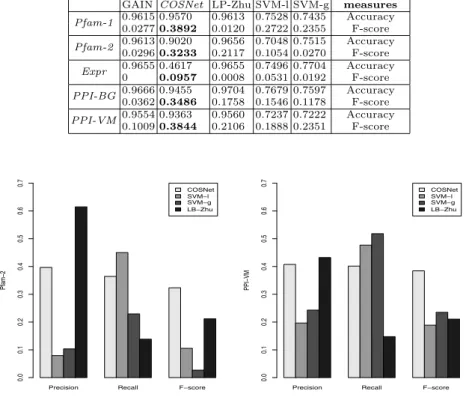
Table 2.Performance comparison between GAIN,COSNet, LP-Zhu, SVM-l, SVM-g
Dataset Methods Performance
GAIN COSNet LP-Zhu SVM-l SVM-g measures
Pfam-1 0.9615 0.95700.02770.3892 0.96130.0120 0.7528 0.74350.2722 0.2355 AccuracyF-score Pfam-2 0.9613 0.90200.02960.3233 0.96560.2117 0.7048 0.75150.1054 0.0270 AccuracyF-score Expr 0.9655 0.46170 0.0957 0.96550.0008 0.7496 0.77040.0531 0.0192 AccuracyF-score PPI-BG 0.9666 0.94550.03620.3486 0.97040.1758 0.7679 0.75970.1546 0.1178 AccuracyF-score PPI-VM0.9554 0.93630.10090.3844 0.95600.2106 0.7237 0.72220.1888 0.2351 AccuracyF-score
Precision Recall F−score
Pfam−2 0.0 0.1 0.2 0.3 0.4 0.5 0.6 0.7 COSNet SVM−l SVM−g LB−Zhu
Precision Recall F−score
PPI−VM 0.0 0.1 0.2 0.3 0.4 0.5 0.6 0.7 COSNet SVM−l SVM−g LB−Zhu
Fig. 1. Average precision, recall and F-score for each compared method (excluding GAIN). Left: Pfam-2; Right: PPI-VM.
informative, since a classifier predicting always “negative” could obtain a very high accuracy. Table 2 shows the average F-score and accuracy across all the classes and for each data set.
The results show that COSNet achieves the best performances (in terms of the F-score) w.r.t. all the other methods. TheLP-Zhumethod is the second best method inPfam-2 and PPI-BG data sets, but obtains very low performances withPfam-1 andExprdata. These overall results are confirmed by the Wilcoxon signed-ranks test [40]: we can register a significant improvement in favour of
COSNet with respect to all the other methods and for each considered data set atα= 10−15significance level.
In order to understand the reasons for which our method works better, we compared also the overall precision and recall of the methods separately for each data set: we did not considerGAIN, since this methods achieved the worst results in almost all the data sets. For lack of room, in Figure 1 we show only the results relative to Pfam-2 and PPI-VM data sets. We can observe that, while
as a result of a good balancing between them. These results are replicated with the other data sets, even if with Pfam-1 and Expr dataCOSNet achieves also the best average precision and recall (data not shown).
We think that these results come from theCOSNet cost-sensitive approach that allows to automatically find the “near-optimal” parameters of the network with respect to the distribution of positive and negative nodes (Section 6). It is worth noting that using only single sources of dataCOSNet can obtain a rela-tively high precision, without suffering a too high decay of the recall. This is of paramount importance in the gene function prediction problem, where “in silico” positive predictions of unknown genes need to be confirmed by expensive “wet” biological experimental validation procedures. From this standpoint the experi-mental results show that our proposed method could be applied to predict the “unknown” functions of genes, considering also that data fusion techniques could in principle further improve the reliability and the precision of the results [2, 41].
8
Conclusions
We introduced an effective neural algorithm,COSNet, which exploits Hopfield networks for semi-supervised learning in graphs.COSNet adopts a cost sensitive methodology to manage the unbalance between positive and negative labels, and to preserve and coherently encode the prior information. We applied COSNet
to the genome-wide prediction of gene function in yeast, showing a large im-provement of the prediction performances w.r.t. the compared state-of-the-art methods.
By noting that the parameterγ of the neural network may assume different values for each node, our method could be extended by allowing a different ac-tivation threshold for each neuron. To avoid overfitting due to the increment of network parameters, this approach should be paired with proper regularization techniques. Moreover, by exploiting the supervised learning of network param-eters,COSNetcould be also adapted to combine multiple sources of networked data: indeed the accuracy of the linear classifier on the labeled portion of the net-work could be used to “weight” the associated source of data, in order to obtain a “consensus” network, whose edges are the result of a weighted combination of multiple types of data.
Acknowledgments. The authors gratefully acknowledge partial support by the PASCAL2 Network of Excellence under EC grant no. 216886. This publication only reflects the authors’ views.
References
[1] Zheleva, E., Getoor, L., Sarawagi, S.: Higher-order graphical models for classifi-cation in social and affiliation networks. In: NIPS 2010 Workshop on Networks Across Disciplines: Theory and Applications, Whistler BC, Canada (2010) [2] Mostafavi, S., Morris, Q.: Fast integration of heterogeneous data sources for
pre-dicting gene function with limited annotation. Bioinformatics 26(14), 1759–1765 (2010)
[3] Vazquez, A., et al.: Global protein function prediction from protein-protein inter-action networks. Nature Biotechnology 21, 697–700 (2003)
[4] Leskovec, J., et al.: Statistical properties of community structure in large social and information networks. In: Proc. 17th Int. Conf. on WWW, pp. 695–704. ACM, New York (2008)
[5] Bilgic, M., Mihalkova, L., Getoor, L.: Active learning for networked data. In: Proc. of the 27th ICML, Haifa, Israel (2010)
[6] Marcotte, E., et al.: A combined algorithm for genome-wide prediction of protein function. Nature 402, 83–86 (1999)
[7] Oliver, S.: Guilt-by-association goes global. Nature 403, 601–603 (2000)
[8] Zhu, X., Ghahramani, Z., Lafferty, J.: Semi-supervised learning with gaussian fields and harmonic functions. In: Proc. of the 20th ICML, Washintgton DC, USA (2003)
[9] Zhou, D.: et al.: Learning with local and global consistency. In: Adv. Neural Inf. Process. Syst., vol. 16, pp. 321–328 (2004)
[10] Szummer, M., Jaakkola, T.: Partially labeled classification with markov random walks. In: NIPS 2001, Whistler BC, Canada, vol. 14 (2001)
[11] Azran, A.: The rendezvous algorithm: Multi- class semi-supervised learning with Markov random walks. In: Proc. of the 24th ICML (2007)
[12] Belkin, M., Matveeva, I., Niyogi, P.: Regularization and semi-supervised learning on large graphs. In: Shawe-Taylor, J., Singer, Y. (eds.) COLT 2004. LNCS (LNAI), vol. 3120, pp. 624–638. Springer, Heidelberg (2004)
[13] Delalleau, O., Bengio, Y., Le Roux, N.: Efficient non-parametric function induc-tion in semi-supervised learning. In: Proc. of the Tenth Int. Workshop on Artificial Intelligence and Statistics (2005)
[14] Belkin, M., Niyogi, P.: Using manifold structure for partially labeled classification. In: Adv. Neural Inf. Process. Syst., vol. 15 (2003)
[15] Nabieva, E., et al.: Whole-proteome prediction of protein function via graph-theoretic analysis of interaction maps. Bioinformatics 21(S1), 302–310 (2005) [16] Deng, M., Chen, T., Sun, F.: An integrated probabilistic model for functional
prediction of proteins. J. Comput. Biol. 11, 463–475 (2004)
[17] Tsuda, K., Shin, H., Scholkopf, B.: Fast protein classification with multiple net-works. Bioinformatics 21(suppl 2), ii59–ii65 (2005)
[18] Mostafavi, S., et al.: GeneMANIA: a real-time multiple association network inte-gration algorithm for predicting gene function. Genome Biology 9(S4) (2008) [19] Hopfield, J.: Neural networks and physical systems with emergent collective
com-pautational abilities. Proc. Natl Acad. Sci. USA 79, 2554–2558 (1982)
[20] Bengio, Y., Delalleau, O., Le Roux, N.: Label Propagation and Quadratic Crite-rion. In: Chapelle, O., Scholkopf, B., Zien, A. (eds.) Semi-Supervised Learning, pp. 193–216. MIT Press, Cambridge (2006)
[21] Karaoz, U., et al.: Whole-genome annotation by using evidence integration in functional-linkage networks. Proc. Natl Acad. Sci. USA 101, 2888–2893 (2004) [22] Ruepp, A., et al.: The FunCat, a functional annotation scheme for systematic
classification of proteins from whole genomes. Nucleic Acids Research 32(18), 5539–5545 (2004)
[23] Wang, D.: Temporal pattern processing. In: The Handbook of Brain Theory and Neural Networks, pp. 1163–1167 (2003)
[24] Liu, H., Hu, Y.: An application of hopfield neural network in target selection of mergers and acquisitions. In: International Conference on Business Intelligence and Financial Engineering, pp. 34–37 (2009)
[25] Zhang, F., Zhang, H.: Applications of a neural network to watermarking capacity of digital image. Neurocomputing 67, 345–349 (2005)
[26] Tsirukis, A.G., Reklaitis, G.V., Tenorio, M.F.: Nonlinear optimization using gen-eralized hopfield networks. Neural Comput. 1, 511–521 (1989)
[27] Ashburner, M., et al.: Gene ontology: tool for the unification of biology. the gene ontology consortium. Nature Genetics 25(1), 25–29 (2000)
[28] Agresti, A., Coull, B.A.: Approximate is better than exact for interval estimation of binomial proportions. Statistical Science 52(2), 119–126 (1998)
[29] Brown, L.D., Cai, T.T., Dasgupta, A.: Interval estimation for a binomial propor-tion. Statistical Science 16, 101–133 (2001)
[30] Cesa-Bianchi, N., Valentini, G.: Hierarchical cost-sensitive algorithms for genome-wide gene function prediction. Journal of Machine Learning Research, W&C Pro-ceedings, Machine Learning in Systems Biology 8, 14–29 (2010)
[31] Eddy, S.R.: Profile hidden Markov models. Bioinformatics 14(9), 755–763 (1998) [32] Spellman, P.T., et al.: Comprehensive identification of cell cycle-regulated genes of the yeast saccharomyces cerevisiae by microarray hybridization. Molecular Biology of the Cell 9(12), 3273–3297 (1998)
[33] Gasch, P., et al.: Genomic expression programs in the response of yeast cells to environmental changes. Mol. Biol. Cell 11(12), 4241–4257 (2000)
[34] Stark, C., et al.: Biogrid: a general repository for interaction datasets. Nucleic Acids Research 34(Database issue), 535–539 (2006)
[35] von Mering, C., et al.: Comparative assessment of large-scale data sets of protein-protein interactions. Nature 417(6887), 399–403 (2002)
[36] Chua, H., Sung, W., Wong, L.: An efficient strategy for extensive integration of diverse biological data for protein function prediction. Bioinformatics 23(24), 3364–3373 (2007)
[37] Lin, H.T., Lin, C.J., Weng, R.: A note on platt’s probabilistic outputs for support vector machines. Machine Learning 68(3), 267–276 (2007)
[38] Brown, M.P.S., et al.: Knowledge-based analysis of microarray gene expression data by using support vector machines. Proceedings of the National Academy of Sciences of the United States of America 97(1), 267–276 (2000)
[39] Pavlidis, P., et al.: Learning gene functional classifications from multiple data types. Journal of Computational Biology 9, 401–411 (2002)
[40] Wilcoxon, F.: Individual comparisons by ranking methods. Journal of Computa-tional Biology 1(6), 80–83 (1945)
[41] Re, M., Valentini, G.: Simple ensemble methods are competitive with state-of-the-art data integration methods for gene function prediction. Journal of Machine Learning Research, W&C Proceedings, Machine Learning in Systems Biology 8, 98–111 (2010)