Target concept learning from ambiguously labeled data

(1)

TARGET CONCEPT LEARNING FROM

AMBIGUOUSLY LABELED DATA

A Dissertation presented to the Faculty of the Graduate School

at the University of Missouri

In Partial Fulfillment

of the Requirements for the Degree Doctor of Philosophy

by Changzhe Jiao

Dr. Alina Zare, Dissertation Supervisor December 2017

(2)

c

(3)

The undersigned, appointed by the Dean of the Graduate School, have examined the dissertation entitled:

TARGET CONCEPT LEARNING FROM

AMBIGUOUSLY LABELED DATA

presented by Changzhe Jiao,

a candidate for the degree of Doctor of Philosophy and hereby certify that, in their opinion, it is worthy of acceptance. Dr. Alina Zare Dr. James Keller Dr. Marjorie Skubic Dr. Dominic Ho Dr. Ronald McGarvey

(4)

ACKNOWLEDGMENTS

I would like to express my special gratitude and thanks to my advisor, Dr. Alina Zare, for her invaluable guidance, support and encouragement throughout my studies and re-search. I would also like to thank my committee members, Dr. James Keller, Dr. Marjorie Skubic, Dr. Dominic Ho and Dr. Ronald McGarvey, for all of their insightful comments and suggestions.

I also want to thank my friends, former and current labmates, particularly to Shanjie Chen, Da Li, Xiaoxiao Du, Hao Sun, Piyush Khopkar and Matthew Cook, for our con-structive discussions during my research work.

(5)

LIST OF TABLES

Table

Page

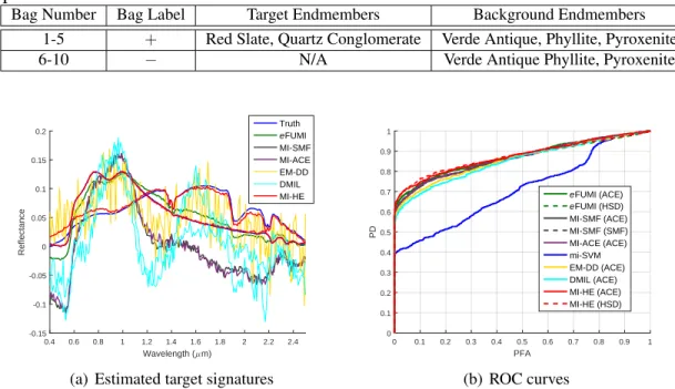
5.1 List of Constituent Endmembers for Synthetic Data with Incomplete Back-ground Knowledge . . . 76 5.2 Detection Statistics (AUCs) for Simulated Hyperspectral Data with

Incom-plete Background Knowledge, Bold for the Best, Underline for the Second Best . . . 80 5.3 List of Constituent Endmembers for Synthetic Data with Multiple Target

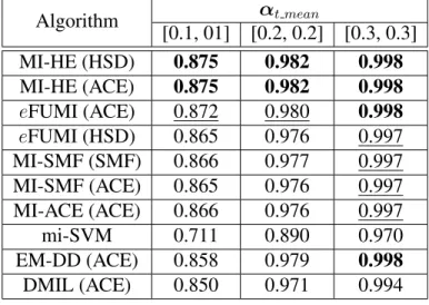
Concepts . . . 82 5.4 Detection Statistics (AUCs) for Simulated Hyperspectral Data with

Multi-ple Target Concepts, Bold for the Best, Underline for the Second Best . . . 84 5.5 List of Constituent Endmembers for Synthetic Data for Parameter

Sensitiv-ity Testing . . . 86 5.6 Detection Statistics (NAUCs) for Gulfport Data with Individual Target Type,

Bold for the Best, Underline for the Second Best . . . 95 5.7 Detection Statistics (NAUCs) for Gulfport Data with All Four Target Types,

(10)

5.8 Errors of MI-HE and Comparisons for Heart Rate Monitoring from 40 Sub-jects, Bold for the Best, Underline for the Second Best . . . 107 5.9 The Correlation Coefficients between Performance and Age, Weight, Height,

BMI and Ground Truth. . . 108 5.10 Tree Species Classification Results (AUCs), Bold for the Best, Underline

(11)

LIST OF FIGURES

Figure

Page

1.1 Illustration of MIL: a molecule with different shapes [1] . . . 2 1.2 Illustration of inaccurate coordinates from GPS: one target denoted as brown

by GPS has one pixel drift. . . 8 1.3 Hydraulic Bed Sensor System. (a) Hydraulic transducer (top) and

embed-ded system (bottom). (b) Transducer placement . . . 10 1.4 BCG signal and ground truth plot . . . 12

2.1 The elim-count procedure for excluding negative instances [1] . . . 20

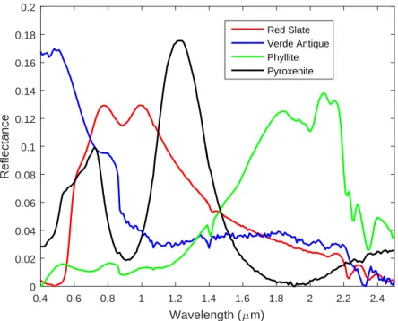
5.1 Signatures from ASTER library used to generate simulated data with in-complete background knowledge . . . 75 5.2 MI-HE and comparisons on synthetic data with incomplete background

knowledge, αt mean = 0.1. MI-SMF and MI-ACE are not expected to

recover the true signature. . . 77 5.3 MI-HE and comparisons on synthetic data with incomplete background

(12)

5.4 MI-HE and comparisons on synthetic data with incomplete background knowledge, αt mean = 0.5. MI-SMF and MI-ACE are not expected to

recover the true signature. . . 78 5.5 MI-HE and comparisons on synthetic data with incomplete background

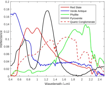
recover the true signature . . . 78 5.6 Signatures from ASTER library used to generate simulated data with

mul-tiple target concepts . . . 81 5.7 MI-HE and comparisons on synthetic data with multiple target concepts,

αt mean = [0.1,0.1]. Not all comparisons algorithms are expected to

re-cover true target signatures. . . 82 5.8 MI-HE and comparisons on synthetic data with multiple target concepts,

re-cover true target signatures. . . 83 5.9 MI-HE and comparisons on synthetic data with multiple target concepts,

re-cover true target signatures. . . 83 5.10 Detection statistics (AUCs) of MI-HE plots with different parameter settings 87 5.11 Plot of exponential functionexp(−β) . . . 88 5.12 MUUFL Gulfport data set RGB image and the 57 target locations . . . 90 5.13 MI-HE and comparisons on Gulfport data Brown, training flight 1 testing

flight 3 . . . 91 5.14 MI-HE and comparisons on Gulfport data Dark Green, training flight 1

(13)

5.15 MI-HE and comparisons on Gulfport data Faux Vineyard Green, training

flight 1 testing flight 3 . . . 92

5.16 MI-HE and comparisons on Gulfport data Pea Green, training flight 1 test-ing flight 3 . . . 92

5.17 MI-HE and comparisons on Gulfport data Brown, training flight 3 testing flight 1 . . . 93

5.18 MI-HE and comparisons on Gulfport data Dark Green, training flight 3 testing flight 1 . . . 93

5.19 MI-HE and comparisons on Gulfport data Faux Vineyard Green, training flight 3 testing flight 1 . . . 94

5.20 MI-HE and comparisons on Gulfport data Pea Green, training flight 3 test-ing flight 1 . . . 94

5.21 ROCs of MI-HE and comparisons on Gulfport data, all types detection. . . . 96

5.22 BCG signal of four transducers and ground truth plot. . . 99

5.23 Plot of one positive bag. . . 100

5.24 Estimated heartbeat concepts by MI-HE. . . 100

5.25 Estimated heartbeat concept by EM-DD. . . 101

5.26 Confidence value and confirmed heartbeats. . . 102

5.27 The Bland Altman plot comparison of MI-HE and EM-DD for Subject No. 10. . . 103

5.28 Heart rate estimation for Subject No. 10. (a) MI-HE (b) EM-DD . . . 104

5.29 RGB image of NEON OSBS with tree polygons . . . 109

5.30 ROC curves of MI-HE and SVM on polygon data . . . 111

(14)

LIST OF SYMBOLS

Symbol Description

x Data vector/instance

N Total number of data vectors/instances

n Number of feature dimensions

X Data matrix,X = [x1,x2,· · · ,xN]

s Target signature/endmember

d Estimated dictionary atom/endmember

·+ _{Superscript for positive/target class}

·− _{Superscript for negative/non-target class}

T Total number of estimated target dictionary atoms/endmembers

·T _{Superscript for Transpose}

M Total number of estimated non-target dictionary atoms/endmembers D Dictionary/endmember matrix, D = [D+_D−_{] = [}_d+ 1,d + 2,· · · ,d + T,d − 1,d − 2,· · · ,d − M]

a Abundance vector or sparse codes ofxcorresponding toD p Abundance vector or sparse codes ofxcorresponding toD− A Sparse codes/proportion matrix,A = [a1,a2,· · ·,aN]

µ Data mean

Σ Data covariance matrix

N Normal distribution

(15)

B Data bag

K Number of data bags

xij jth instance from theith bag

L Bag-level label

l Instance-level label

w Weights for a linear classifier

C Total number of classes

W Weights matrix for a multi-class linear classifier, W= [w1,w2,· · · ,wC]

δ Step length for gradient descent

Λ(x) Detector response ofx

0n×1 Column vector with numbern0elements

11×M Row vector with numberM 1elements

A B

Concatenating of arraysAandBhorizontally    A B  

 Concatenating of arraysAandBvertically

RN(a) = [a,· · · ,a]1×N Matrix containing repeated entries ofa

with repetition ofN vectors

(16)

LIST OF ACRONYMS

Acronym Description

MIL Multiple Instance Learning

eFUMI Extended FUnctions of Multiple Instances

DL-FUMI Dictionary Learning using FUnctions of Multiple Instances SVM Support Vector Machine

mi-SVM mixed-integer SVM (instance-level) MI-SVM Mixed-Integer SVM (bag-level) SMF Spectral Matched Filter

ACE Adaptive Coherence/Cosine Estimator HD/HSD Hybrid Detector/Hybrid Structured Detector

K-SVD Dictionary Learning using Singular Value Decomposition GPS Global Positioning System

EM Expectation Maximization

DD Diverse Density

EM-DD Diverse Density using Expectation Maximization MI-HE Multiple Instance Hybrid Estimator

GLRT Generalized Likelihood Ratio Test

HBS Hydraulic Bed Sensor

BCG Ballistocardiogram

ECG Electrocardiography

BMI Body Mass Index

PD Probability of Detection

(17)

PFA Probability of False Alarm FCLS Fully Constrained Least Squares APR Axis-Parallel Rectangles

DMIL/GDMIL Dictionary based Multiple Instance Learning/

Generalized Dictionaries for Multiple Instance Learning MILES Multiple-Instance Learning via Embedded Instance Selection VCA Vertex Component Analysis

ISTA Iterative Shrinkage Thresholding Algorithm AUC/NAUC Area Under Curve/ Normalized Area Under Curve ROC Receiver Operating Characteristic

(18)

ABSTRACT

The multiple instance learning problem addresses the case where training data comes with label ambiguity,i.e., the learner has access only to inaccurately labeled data. For ex-ample, in target detection from remotely sensed hyperspectral imagery, targets are usually sub-pixel and the ground truthing of the targets according to GPS coordinates could drift across several meters. Thus the locations of the targets corresponding to the hyperspec-tral image are inaccurate. Training a supervised algorithm or extracting target signatures from this kind of labels is intractable. This dissertation investigates the topic target concept learning from ambiguously labeled data comprehensively; reviews and proposes several methods that either learn a set of representative or discriminative target concepts.

The multiple instance hybrid estimator (MI-HE) maximizes the response of the hybrid detector under a generalized mean framework and estimates a set of discriminative target concepts. MI-HE adopts a linear mixture model and iterates between estimating a set of discriminative target and non-target signatures and solving a sparse unmixing problem. MI-HE preserves bag-level label information for each positive bag and is able to estimate a target concept that is commonly shared among positive bags. Furthermore, MI-HE has the potential to learn multiple signatures to address signature variability.

After learning target concept, signature based detector could be applied for target de-tection. The presented algorithms were tested in many applications including simulated and real hyperspectral target detection, heartbeat characterization from ballistocardiogram signals and tree species classification from remotely sensed data. The presented algo-rithms were proven to be effective in learning high-quality target signatures and consis-tently achieved superior performance over the state-of-the-art comparison algorithms.

(19)

Chapter 1 Introduction

In supervised learning, each training data is assumed to be coupled with the desired classifi-cation output. However, acquiring accurately labeled training data can be time consuming, expensive and even infeasible. Furthermore, labeling ambiguity comes naturally in many machine learning and computer vision applications, for example, an image that is labeled as computer may also contain a desk or several books; a video that is labeled as abnormal may only have its subset frames containing an accident, making the training label ambigu-ous [2, 3].

In hyperspectral target detection [4, 5], ground truth label information coming from a GPS receiver could drift across several pixels depending on the accuracy of the GPS, thus it is only known that some area denoted by the ground truth contains some points of interest for sure. In medical applications like heartbeat characterization and heart rate estimation from Ballistocardiogram (BCG) signals [6–8], ground truth is not strictly aligned in time with the BCG signals and moreover, there may be some missed collection of heartbeat sig-nals by the BCG sensors. These labeling uncertainties make traditional supervised learning

(20)

Rotated Bond

Figure 1.1: Illustration of MIL: a molecule with different shapes [1]

algorithms challenging to apply and the multiple instance learning algorithms more appeal-ing.

Multiple instance learning (MIL) problem was first comprehensively investigated by Dietterichet al. [1] in the 1990s for the prediction of drug activity (musk activity). The effectiveness of a type of drug is determined by how tightly the drug molecule binds to a much larger protein molecule (eg., enzymes and cell-surface receptors). However, a certain molecule determined by laboratory assay to be effective can have alternative variants called “conformations” - different structures the molecule could be by rotating its bonds shown by Fig. 1.1. Among all those different conformations the effective molecule could adopt, only one (or a few) actually binds to the desired target binding site. The learning task is to infer the correct shape of that molecule that actually has tight binding capacity.

In order to solve this problem, Dietterichet al. introduced the concept of “bags”. Each molecule was treated as a bag and each possible conformation the molecule could be was treated as an instance in that bag. This directly induces the definition of multiple instance learning problem: a positively labeled bag contains at least one positive instance and

(21)

neg-atively labeled bags are composed of entirely negative instances. Finally, Dietterich et al. proposed to solve this problem by finding axis-parallel rectangles constructed by the conjunction of the features as approximation of the binding conformation.

Dietterich et al. also compared the proposed algorithm with several classical super-vised learning algorithm including the backpropagation neural network and decision tree, and concluded that any supervised machine learning algorithm will perform poorly on MIL problem without considering the essence of MIL. Since Dietterich’s work, many MIL learn-ing algorithms were proposed and investigated. The MIL algorithms in the literature can be generally divided into two categories: learning an individual or a set of concepts that describe the positive class or learning a classifier that is able to classify individual instances or bags. This dissertation focuses on the former category, learning an individual or a set of concepts that either try to describe the positive class or distinguish the positive instances. Here, concepts refer to generalized class prototypes in the feature space.

1.1 Hyperspectral Image Analysis

Hyperspectral imaging spectrometers (also referred to as hyperspectral sensors) collect electromagnetic energy scattered in the scene across hundreds or thousands of spectral bands, and thus capture both the spatial and spectral information [9]. The spectral infor-mation is a combination of the reflection and/or emission of sunlight across wavelength by objects on the ground, and contains the unique spectral characteristics of different materials [10, 11]. The wealth of spectral information in hyperspectral imagery enables the possibil-ity to conduct sub-pixel analysis including target detection [12, 13], precision agriculture [14, 15], biomedical applications [16, 17] and others [11, 18, 19].

(22)

1.1.1 Hyperspectral Image Data

Hyperspectral cameras collect radiance data over a high resolution range of wavelength, typically in the range of 0.3µmto 2.5µm[20] and construct a three-dimensional data cube. In hyperspectral data cube, each layer corresponds to a certain band of wavelength over all pixels and each pixel corresponds to the radiance value at certain location over the entire spectral bands. Due to the spatial resolution of hyperspectral cameras and high diversity of nature scene, individual pixel may be a mixture of several objects, in other words, each pixel may contain several different materials, called endmembers. Endmembers are assumed spectral value vectors over the wavelength for the pure materials present in the image. But the definition of “pure materials” could be also task driven or user defined.

As each pixel is a mixture of endmembers, abundances or proportions, are the amount or percentage of each endmember presents in an individual pixel. The magnitude of each endmember’s proportion in an individual pixel is determined by many factors, e.g., the relative area of the corresponding object, reflective intensity of materials, interactive ab-sorption and scattering of light. Beside this, how the mixture is modeled also matters. Both linear and non-linear mixture models have been developed and verified to be effective in different physical context in the literature [11]. In realistic, the spectral mixture in remote sensing should be non-linear, due to the multiple mixture of light among different objects on the ground, e.g., between tree canopy and the ground, and microscopic scattering be-tween molecules. However, the linear mixing model that assumes each pixel is a convex combination of endmembers and proportions maintains the advantages of simplicity and good generalization ability and is investigated and adopted immensely. This dissertation mainly focuses on the linear mixing model.

(23)

1.1.2 Hyperspectral Unmixing

Hyperspectral unmixing can be decomposed into two major tasks: endmember estimation

andabundance estimation. A mixing model needs to be assumed before conducting

spec-tral unmixing. The convex mixing model assumes each pixel is a convex combination of the endmembers, xj = M X k=1 ajkdk+εj, j = 1, . . . , N (1.1) M X k=1 ajk = 1, ajk ≥0,∀j, k, (1.2)

whereN is the total number of data points,M is the number of endmembers (or materials), xj is the spectral value of the jth data point, εj is an error/noise term, dk is the spectral

signature of the kth endmember, and ajk is the abundance of the jth pixel corresponding

to the kth endmember. The abundances in this model are constrained to the sum-to-one and non-negative constraint shown in Eq. (1.2). Typically, only the N data points are known as the input hyperspectral image, the remaining variables in the model including the spectral value of the endmembers, the number of endmembers,M, and corresponding abundance values are unknown and need to be solved. Estimating these unknown variables is an ill-posed inverse problem.

Many unsupervised hyperspectral unmixing methods adopt a number of assumptions about hyperspectral imagery to solve the ill-posed problem [10, 21–25]. For example, these methods include requiring the solution of endmembers to be found within the input data [26–31], adding volume penalty [32–35], assuming sparsity constraints [36–41], or adding the spatial smooth constrain on the abundance values [42–46]. These hyperspectral unmixing methods are mainly unsupervised algorithms. However, it is more appealing to

(24)

apply supervised or task driven unmixing [47, 48] if prior information about the particular materials of interest is available.

1.1.3 Hyperspectral Target Detection

Hyperspectral target detection generally refers to the task of locating all instances of a target given a known spectral signature within a hyperspectral scene. A large number of hyperspectral target detection methods have been developed in the literature [4, 5, 49, 50]. The reasons most classification methods are not applicable to hyperspectral target detection tasks are threefold:

1. The number of training instances from the positive (target) class is small compared to that of the negative training data such that training an effective classifier is difficult. Typically in a hyperspectral image with size hundreds by hundreds pixels, there are only a few pixel or sup-pixel level target points. Compared with the number of the non-target points, this number of target points is too few to effectively train an classifier,e.g., a SVM may be biased by the excessive non-target points and achieves very high classification accuracy but low detection rate.

2. Due to the relatively low spatial resolution of hyperspectral imagery and the diversity of natural scenes, many targets are mixed points (sub-pixel targets). Most of the supervised learning algorithms assume each training data is a prime prototype of a class denoted by the label paired with this data. However, in hyperspectral image, a target pixel could be a mixture of several background materials and the amount of target mixture is unknown. Supervised learning algorithms will be stuck without considering the fact of mixture in training data.

(25)

3. Precise training labels are often difficult or infeasible to obtain. In hyperspectral im-age analysis, the ground truth information usually comes from a Global Positioning System (GPS) receiver placed to the target. However, the co-registration of the tar-gets in the image to the GPS coordinates could drift for several meters. That means a target pixel denoted by the GPS coordinates could be a false positive point. The only reliable knowledge is with in a certain region there exists some targets for sure.

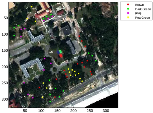
As an example, Fig. 1.2(a) shows the scattered target locations over MUUFL Gulf-port data set collected over the University of Southern Mississippi-Gulfpark Campus [51], where there are 4 types of targets throughout the scene: Brown (15 examples), Dark Green (15 examples), Faux Vineyard Green (12 examples) and Pea Green (15 examples). The highlighted region shown in Fig. 1.2(a) is one of the brown target locations whose zoomed view is shown in Fig. 1.2(b), where we can clearly see that for this brown target there is one pixel drift between the real target location and ground truth location given by GPS. De-veloping a classifier or extracting a pure prototype for the target class given this incomplete knowledge of the training data is intractable, thus MIL methods are needed.

(26)

50 100 150 200 250 300 50 100 150 200 250 300 Brown Dark Green FVG Pea Green

(a) Scattered target locations over MUUFL Gulfport data set

173.5 174 174.5 175 175.5 176 176.5 177 177.5 178 178.5 219.5 220 220.5 221 221.5 222 222.5 223 223.5 224 224.5 Brown Dark Green FVG Pea Green

(b) Zoomed region of one target

Figure 1.2: Illustration of inaccurate coordinates from GPS: one target denoted as brown by GPS has one pixel drift.

(27)

1.2 Ballistocardiogram Signal Analysis

Long-term measurement and monitoring of vital signs, e.g., heart rate, respiratory rate, body temperature and blood pressure, provides promise for the early treatment of any potential problems, especially for older adults. Compared with the many wearable heart rate monitoring systems available, ballistocardiography provides an unobtrusive and, thus, comfortable monitoring alternative. These systems record the motion of the human body generated by the sudden ejection of blood into the large vessels at each cardiac cycle [6]. Such motion contains rich information and has gained revived interest due to recent de-velopment in measurement technology [7, 8] and a growing interest in managing chronic health conditions through passive sensors in the home [52].

1.2.1 Hydraulic Bed Sensor System

The hydraulic bed sensor (HBS) developed at the Center for Eldercare and Rehabilitation Technology (CERT) at the University of Missouri is a BCG device providing a low-cost, noninvasive and robust solution for capturing physiological parameters during sleep [53– 55]. The HBS was designed to maintain an imperceptible flat profile and to be used beneath a bed mattress. The system is comfortable for subjects lying on the mattress (i.e., nonin-vasive), easy to install, watertight, and durable. Compared with other methods such as electrocardiography (ECG), BCG does not need electrodes or clips to be affixed to the patient’s body and thus is ideal for long term in-home monitoring. However, the lack of saliency and large variability in a BCG signal makes it much more difficult to detect indi-vidual heartbeats than with an ECG.

(28)

(a) Sensor and Embedded System

(b) Transducer placement

(29)

transducer was designed to be placed under the subject’s upper torso. It is 54.5 cm long, 6 cm wide, and is filled with 0.4 liters of water [53–55]. The integrated silicon pressure sensor (Freescale MPX5010GP) attached to the end of the transducer is used for measuring the vibration of human body arising from each heartbeat. It captures the information of heartbeat together with respiration and motion artifact. The signal from each transducer is then amplified, filtered and sampled at 100 Hz. For ground-truthing, a piezoelectric pulse sensor (TN1012/ST, ADInstruments) attached to subject’s finger was used to record the pulse ejected by a heartbeat.

In order to ensure enough coverage, four transducers are placed in parallel underneath a mattress as shown in Fig. 1.3(b). The four transducers are identical and independent, but the data quality collected by those four transducers could vary depending on the sleeping position, type of mattress (e.g., material, thickness) and the physical characteristics of the subject (e.g., age, body mass index (BMI)).

1.2.2 Multiple Instance Learning Problem in Ballistocardiograms

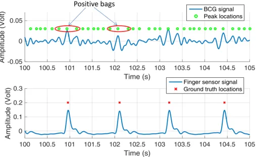
Fig. 1.4 shows a typical filtered BCG signal collected by one transducer and the corre-sponding finger sensor ground truth information, where the green circles denote every peak location of the filtered BCG signal. From Fig. 1.4, it can be seen that near the ground truth locations denoted by the finger sensor, there are prominent peak patterns measured by the BCG transducer corresponding to heartbeats. However, although all of the sensors are expected to be capturing each corresponding heartbeat signal simultaneously, there is unavoidable misalignment between the finger sensor and each of the BCG pressure sensors. Furthermore, depending on the location and position of the subject lying on the bed, which of these BCG sensors are able to capture a clear heartbeat signal is difficult to determine.

(30)

Positive bags

Figure 1.4: BCG signal and ground truth plot

These multiple labeling uncertainties in the training data cast more difficulties to traditional supervised learning methods for heartbeat detection and heart rate estimation from a BCG signal.

For this problem, this dissertation proposes to introduce the idea of training “bags” to address label uncertainty as well as mis-collection of heartbeat signals in the BCG data. So accurately labeled BCG signals are no longer needed. The proposed MI-HE algorithm is expected to learn a set of discriminative subject-specific heartbeat concepts from training bags of this type. After learning the heartbeat concept, a signature based detector can then be applied for real-time heartbeat monitoring and heart rate estimation.

(31)

1.3 Signature Based Detectors

The majority of sub-pixel detection techniques are statistical methods in which the target and background signals are modeled as random variables distributed according to some respective underlying probability distribution [4, 56, 57]. The detection problem can then be posed as a binary hypothesis test with two competing hypotheses: target absent (H0) or

target present (H1) and a detector can be designed using the generalized likelihood ratio

test (GLRT) approach [58]. Following the Neyman-Pearson criterion that maximizes the probability of detection (PD) given any desired probability of false alarm (PFA), the GLRT is shown in Eq. (1.3), Λ(x) = f(x|Target present) f(x|Target absent) , f(x|H1) f(x|H0) H1 ≷ H0 η, (1.3)

wheref(x|Hi)is the likelihood function value for each hypothesis.

1.3.1 Spectral Matched Filter

The hypotheses used for the spectral matched filter (SMF) [4, 58–61] are:

H0 :x∼ N(0,Σb)

H1 :x∼ N(as,Σb) (1.4)

whereΣbis the background covariance andsis the known target signature which is scaled

(32)

the SMF detector: ΛSM F(x,s) = sT_Σ−1 b (x−µb) q sT_Σ−1 b s (1.5)

where µb is the background mean subtracted from the data to ensure a zero-mean

back-ground as defined inH0.

1.3.2 Adaptive Coherence/Cosine Estimator

The hypotheses used for the structured-background adaptive coherence/cosine estimator (ACE) [62–64] are: H0 :x∼ N 0, σ02Σb H1 :x∼ N as, σ12Σb (1.6) which includesσ2 0 = 1nx T_Σ−1 b xandσ21 = 1n(x−as) T Σ−_b1(x−as)to add scale-invariance to the ACE detector wheren is the dimensionality of the spectra. The square-root of the GLRT for (1.6) results in the following as the ACE detector [62, 63]:

ΛACE(x,s) = sT_Σ−1 b (x−µb) q sT_Σ−1 b s q (x−µb)TΣb−1(x−µb) . (1.7)

Compared with Eq. (1.5), the ACE detector can be viewed as a normalized version of SMF: the input test points are whitened and normalized before the projection to the target signature. The normalization step removes the magnitude difference from the input data and achieves better performance in some scenarios, e.g., test data with large variance in

(33)

magnitude.

1.3.3 Hybrid Detector

The hypotheses used for the background structured hybrid detector (HSD) [56, 65] are:

H0 :x∼ N D−p, σ02Σb

H1 :x∼ N Da, σ12Σb

(1.8)

whereD and D− represent the full endmember set and background endmembers set, re-spectively. aandpare the abundance values computed by Fully Constrained Least Squares (FCLS) [66] corresponding toDandD−, respectively. The GLRT for (1.8) results in HSD detector: ΛHSD(x,D) = (x−D−p)T_Σ−1 b (x−D −_p₎ (x−Da)T_Σ−1 b (x−Da) , (1.9)

The hybrid detector models the reconstruction error of each point as a zero mean Gaus-sian distribution using the entire endmember set and non-target endmember set, respec-tively. The ratio between the reconstruction error using the entire endmember set and only the non-target endmember escalates the difference in the two reconstruction errors. The hy-brid detector explicitly models the mixture in hyperspectral data and provides a sub-pixel detection alternative.

(34)

1.4 Overview of Research

In this dissertation, algorithms for target characterization (i.e., estimation of target concept signatures) from training data with labeling ambiguity are presented. The goal of these algorithms are to estimate the target concept signatures from mixed training data that are effective for a follow-on target detection task. Since these algorithms extract the concept signatures from training data, then the background materials, environmental and atmo-spheric conditions, and other such variables are addressed during target characterization.

In the following, Chapter 2 provides a literature review of current multiple instance concept learning approaches and classifier learning approaches respectively. Chapter 3 in-troduces four previously proposed target concept learning algorithms: extended function of multiple instances (eFUMI) [67–70], dictionary learning using function of multiple in-stances (DL-FUMI) [71, 72], multiple instance spectral matched filter (MI-SMF) and mul-tiple instance adaptive coherence/cosine estimator (MI-ACE) [73]. Chapter 4 investigates learning discriminative target concepts from MIL problem by maximizing the Hybrid De-tector and proposes the multiple instance hybrid estimator (MI-HE) [74, 75]. Chapter 5 conducts a comprehensive testing of MI-HE and compares with previously proposed algo-rithms and the state-of-the-art MIL algoalgo-rithms. Chapter 6 provides a conclusion and future work.

1.5 Formulation

Without loss of generality, letX = [x1,· · · ,xN] ∈ Rn×N be training data wheren is the

dimensionality of an instance andN is the total number of training instances. The data are grouped into K bags, B = {B1, . . . ,BK}, with associated binary bag-level labels, L =

(35)

{L1, . . . , LK}whereLi ∈ {0,1}; Ni is the number of instances in bag Bi andxij ∈ Bi

denotes thejth instance in bagBi with instance-level labellij ∈ {0,1}. When identifying

the label on a certain bag or instance is important, theN training data are assumed to be partitioned into K+ _{positive bags with total number of instances} _N+_{, and} _K−

negative bags with total number of instancesN−. ThusN =N+₊_N− ₌PK+

i=1Ni+

PK++K−

i=K+₊₁Ni

whereNiis the number of instances for theith bag. A positive bag will be indicated asB+i

with associated bag level labelLi = 1 containing instancesxij with instance-level labels

lij, s.t.

PNi

j=1lij ≥ 1. Similarly, B−i denotes a negative bag with bag level label Li = 0

(36)

Chapter 2 Literature Review

This chapter provides a review of existing MIL algorithms discussed into two categories, multiple instance concept Learning and multiple instance classifier Learning, respectively.

2.1 Multiple Instance Concept Learning

Multiple instance concept learning refers to learning a description for the positive class given the bag-level labeled training data from MIL problem. Normally some prior knowl-edge is assumed in this step,e.g., the estimated concept should be close to least one instance in each positively labeled bag and far away form every instance in the negatively labeled bags; the estimated concept must be a bad representation of all the negative instances. The estimated target concepts have the physical meaning to tell the unique features for the pos-itive class and can be applied for further applications,e.g., classification or regression.

(37)

2.1.1 Axis-parallel Rectangles

The Axis-parallel Rectangles (APR) [1] algorithms were proposed by Dietterichet al. for drug activity prediction in the 1990s. An axis-parallel rectangle can be viewed as an over-lap or aggregation region of true positive instances in the feature space. In APR algorithms, a lower bond and upper bond are estimated for the scope of positive (active) class. Three APRs, GFS elim-count (greedy feature selection elimination count), GFS kde (greedy fea-ture selection kernel density estimation) and iterated-discrim (iterated discrimination) al-gorithms were investigated and compared in [1].

GFS elim-count APR

The GFS elim-count APR refers to finding an APR in a greedy manner starting from the inclusion of all positive instances. This algorithm first finds the “all-positive APR” that exactly covers all of the positive instances. Fig. 2.1 shows the “all-positive APR” as a solid line bounding box of the instances, where the unfilled markers represent feature vectors of active instances and filled markers represent negative instances. As shown in the figure, the all-positive APR may contain several negative examples. The next step is to eliminate those negative instances and keep the positive instances as many as possible. A greedy shrinkage procedure was performed, which first excludes the “cheapest” negative instance by counting the minimum number of positive instances that needs to be removed from the APR for each negative instance. The greedy algorithm iteratively excludes the negative instance with the least cost (i.e., the negative instance associates with the least positive instance to be removed) until all negative instances within the all-positive APR are eliminated. The dashed box in Fig. 2.1 indicates the final shrinkage APR by elim-count.

(38)

ex-2 2 2 2 1 1 4 𝑋2 𝑋1

(39)

tracted by measuring the length of rays emanating from the origin of each instance (musk molecule) and nearby rays could be highly correlated. Also it is possible that only a sub-set of the feature dimensions is discriminative. So after constructing this shrinkage APR, the greedy feature selection algorithm that iteratively selects the feature dimensions that eliminates the most negative instances is conducted until no negative instance remain to be eliminated.

The GFS elim-count APR eliminates all negative instances from itself but one problem with this method is it is not guaranteed to contain at least one positive instance for each positive bag.

GFS kde APR

In order to solve the problem that GFS elim-count APR cannot preserve at least one positive instance for each positive bag, the author proposed to introduce a Gaussian kernel density estimate (kde) function to assign a cost value to each positive instance associated with the negative instance to be removed, GFS kde APR, instead of merely counting the number of positive instances must be eliminated for removal of one negative instance.

The proposed cost function is shown in Eq. (2.1), whereGd(xij)is the Gaussian kernel

density estimation denoting the probability of observingxij. The cost function (2.1) adds

three criteria to a positive instance associated with a negative instance to be removed:

1. The cost of removingxij should be small if there are many other positive instances

xik, k= 1,· · ·Ni, k 6=j, surviving in bagB+i .

2. xij should be eliminated if there are many other positive instances are also observed

(40)

3. Assign a low cost value ifxij is very isolated, i.e., there are few other positive

in-stances located nearxij in the feature space.

− Ni X k=1,k6=j Gd(xij) ! +αGd(xij) (2.1)

According to Eq. (2.1), the last positive instance in each positive bag will be added by a very large cost value to not be eliminated. To some degree this “outside-in” method keeps the notion of MIL to have at least one positive instance per positive bag. However, one drawback of this algorithm is the computation complexity. It is quite expensive to compute every necessary kernel density estimates, e.g., each negative instance may associate with several positive instances to be excluded across each of the n dimensions.

Iterated Discrimination APR

The iterated-discrim APR is an “inside-out” algorithm and tries to find the smallest APR that contains at least one instance per positive bag. It first choses an initial “seed” positive instance and iterates between two steps, growing a tight APR and selecting discriminat-ing features until convergence, and then performs an expenddiscriminat-ing procedure to improve its generalization ability, described as follows:

1. In this growing a tight APR step, the author proposed a cost function to define the size of an APR shown as Eq. (2.2), which is the sum of all its side length, where n is the index of feature dimension and ubn and lbn is the upper bond length and

lower bond length of nth dimension, respectively. This cost function is optimized by a greedy algorithm to incorporate the “cheapest” positive instance followed by a

(41)

back-fitting algorithm [76] that tunes back at each greedy step.

Size(AP R) =X

n

ubn−lbn (2.2)

2. In this feature selection step, the algorithm iteratively choose feature that “strongly discriminates” the most number of negative instances. Here the “strongly discrimi-nate” is defined either if one negative instance lies more than 1 ˚A outside the bounds of the APR for feature dimensionnor if one negative instance lies beyond the bounds of the APR and lies further along featurenthan along any other dimensions.

After iteration between step 1 and 2 (which is said to converge within 3-4 iterations), a too tight, sub-dimensional APR that excludes most positive instances was esti-mated. So a kernel density estimation method was adopted to expand this tight APR to include more positive instances which made the resulted APR a more generalized concept region. The iterated-discrim APR was verified to have the best performance on the musk dataset. However, one problem with the iterated-discrim APR is in theory the resulted APR may contain a subset of instances belong to negative bags.

2.1.2 Diversity Density

Diversity Density (DD) [2, 77] tries to learn a concept for the positive class that is close to the intersection of positive bags and far always from every negative instance,i.e., an area preserves both high density of target points and low density of non-target points, called diversity density.

The proposed general maximum likelihood function by DD is shown in Eq. (2.3), wheresis the assumed true concept for the positive class anddis the concept variable for

(42)

estimation, arg max d K+ Y i=1 Pr(d=s|B+_i ) K+₊_K− Y i=K+₊₁ Pr(d=s|B−_i ) (2.3)

Each term in the likelihood function Eq. (2.3) was defined by the noisy-or model,

The casual probability for individual instance is modeled by the distance between the individual instance and the positive concept location,

Pr(d=s|xij) = exp(−kxij −dk2). (2.6)

The intuitive understanding of the proposed noisy-or model is if there is at least one in-stance in positive bagB+_i is close todthenPr(d=s|B+_i )is high; thus the first term in the noisy-or model in Eq. (2.4) makes sure that the estimated dclose to at least one instance in every B+_i . Eq. (2.5) drives the estimatedd to be far away from every instance in B−_i . Similarly as stated in [1], a band selection was performed by optimization of the weights added to each dimension.

As stated by the author, the noisy-or model is highly non-smooth and there are several local maxima in the solution space which make finding the global optima very difficult. Gradient ascent with starting points from every positive instance was adopted to maximize the proposed log-likelihood function. Although it showed competitive performance to the comparison algorithms, the computational complexity is still a problem.

(43)

2.1.3 Expectation Maximization of Diversity Density

An expectation maximization version of Diversity Density (EM-DD) [78] was proposed by Zhang et al. in order to improve the computation time of DD [2, 77]. EM-DD assumes there exists only one instance per bag corresponding to the bag-level label and treats the knowledge of the key-point instance corresponding to the bag-level babel as a hidden latent variable. EM-DD starts with some initial guessing of the positive conceptdand iterates be-tween an expectation step (E-step) that picks one point per bag as the representative point of that bag and then performs a quasi-newton optimization (M-step) [79] on the single-instance DD problem. In more detail, in the E-step, the probability of each single-instance to be the one determines the bag-level label given target concept d from the previous iteration is estimated by a multivariate Gaussian distribution as shown in Eq. (2.7), wherex∗_i is the assumed representative instance for bagBi. In the M-step, the positive conceptd0 is

esti-mated by optimizing the standard DD problem with only one instance per bag determined in the E-step, shown in Eq. (2.8), where Pr(Li|d,x∗i)is the reduced single instance DD

problem from Eq. (2.3).

x∗_i = arg max xij∈Bi exp(−kxij −dk2) (2.7) d0 = arg max d Y i Pr(Li|d,x∗i) (2.8)

It was stated in the original paper “EM-DD runs over 10 times faster than DD on Musk 1 and over 100 times faster when applied to Musk2” [78] and achieved the highest accu-racy (above 95%) over the comparison algorithms by picking specific initialization using validation data. However, EM-DD was later verified in [80] to have close but inferior

(44)

performance to DD.

2.1.4 Dictionary based Multiple Instance Learning

Dictionary based Multiple Instance Learning (DMIL) [81] and its generalization, General-ized Dictionaries for Multiple Instance Learning (GDMIL) [82], propose to optimize the noisy-or model using dictionary learning methods [83–87]. The target concept estimated is a set of dictionary atoms. In detail, the author models the probability of individual instance to be positive as a zero-mean multi-variate Gaussian distribution of the reconstruction error between the individual instance and the linear combination of positive dictionary atoms, shown as Eq. (2.9), wherepij is the probability for instancexij to be a true positive point;

Dis the estimated dictionary set as the positive concept set andaij is the sparse

represen-tation ofxij givenD,

pij ∝exp(−kxij −Daijk22). (2.9)

Given the model defined in Eq. (2.9), the modified noisy-or model to be optimized is shown in Eq. (2.10) and the negative logarithm of Eq. (2.10) is shown in Eq. (2.11), where αis a scaling term to control the influence of negative bags.

J(D,X) = K+ Y i=1 1− Ni Y j=1 (1−pij) !_K+₊_K− Y i=K+₊₁ Ni Y j=1 (1−pij) ! (2.10) −logJ(D,X) =− K+ X i=1 log 1− Ni Y j=1 (1−pij) ! −α K+₊_K− X i=K+₊₁ Ni X j=1 log(1−pij) (2.11)

(45)

between two steps, a dictionary learning step that solves the dictionaryD atom by atom using gradient descent method and a sparse coding step that solves the sparse representation of each instance in X given current dictionaryD using orthogonal matching pursuit [88, 89].

The advantages of DMIL over the past multiple instance concept learning algorithms lie in two folds:

1. Instead of learning one concept for the positive class, DMIL learns a set of positive dictionary atoms to better describe the positive class.

2. The second term in the negative log-likelihood function,−αP

i:Li=−

PNi

j=1log(1−

pij), enforces that the negative instances are all poorly represented by the estimated

dictionary D, so that D maintains discriminative features of the positive class and contains the least information from the negative class.

2.2 Multiple Instance Classifier Learning

Multiple instance classifier learning refers to training a discriminative model from labeled training bags in MIL problem for prediction the label of unknown bags or individual in-stances. Since the positive bags are mixture of both positive and negative data, the multiple instance classifier learning algorithms in the literature typically train a classifier through a heuristic way,i.e., starting from some initial guessing of the labels for data from positively labeled bags.

(46)

2.2.1 Mixed Integer Support Vector Machine

Andrews et al. model the MIL problem as a generalized mixed integer formulation of support vector machine [90] algorithms (mi-SVM and MI-SVM). The two proposed al-gorithms lead to mixed integer quadratic programming problem and were solved through heuristic ways. The two algorithms mi-SVM and MI-SVE differ in the manner of selection of training data. mi-SVM adopts the entire training data into consideration to train a SVM and modifies the instance-level label iteratively; whereas the MI-SVM trains a SVM by se-lecting one instance per bag with the maximum classification confidence as representative instance of each bag. The two algorithms stop when there is no change in the assigned label to instances across two iterations. mi-SVM and MI-SVM assume the labels for the training data are subject to the following MIL constraint shown in Eq. (2.12):

X

xij∈Bi

lij + 1

2 ≥1, ∀i s.t. Li = 1, andlij =−1, ∀i s.t. Li =−1 (2.12)

mi-SVM

The mi-SVM tries to solve a soft-margin maximization problem jointly over the possible labels assigned to individual instances and the hyperplane. The formulation of mi-SVM is shown in Eq. (2.13). min {lij} min w,b,ξij 1 2kwk 2 ₊_α N X i=1 ξij s.t.∀i:lij(hw,xiji+b)≥1−ξij, ξij ≥0, lij ∈ {−1,1}, and (2.12) holds, (2.13)

(47)

where(w, b)are the weights and bias for a SVM classifier,ξij is a slackness term andαis

the scaling factor for slackness.

The problem of optimizing Eq. (2.13) is the accurate values of alllij from positive bags

are not known. In order to solve this mixed-integer quadratic programming problem, the author adopted a heuristic optimization strategy. Specifically, the labellij for each instance

from positive bags was initialized by generalizing the bag-level labelLi to individual

in-stance,lij = Li,for Li = 1. Then a SVM was trained and applied to the positive training

bags again to reset its instance-level label. If any of the positive bag has its all instances classified into negative,i.e.,P

xij∈B+i(1 +lij)/2 == 0, the instance in this bag with

max-imum confidence value to be positive will be assigned a positive label and a SVM was trained again based on the newly reset labels. The algorithm stops until there is no change in the instance-level label.

The mi-SVM starts from all instances from positive bags with label 1and iteratively modifies the labels according to the bag constraint in MIL problem until there is no change in label re-assignment. It finally looks for a MI-separating hyperplane such that each posi-tive bag has at least one of its instances is classified into posiposi-tive and all negaposi-tive instances are separated to the other side of the hyperplane. However, there is no guarantee that this process will converge.

MI-SVM

Another way to applying max-margin optimization to mixed integer SVM is to generalize the notion of margin to be maximized from individual instances to bags. The functional margin for each bag,γI, is defined by the maximum decision values of the entire instances

(48)

decision value in each bag are adopted to train a SVM. One thing to notice is the margin of a positive bag is defined by the “most positive” instance, whereas the margin of a negative bag is defined by the “least negative” instance.

γi ≡Li max xij∈Bi

(hw,xiji+b) (2.14)

The formulation of MI-SVM is shown in Eq. (2.15), where ξi is the slackness for bag

Bi. MI-SVM is initialized by assigning the mean of each bag as its representative

train-ing instance and optimized alternatively between traintrain-ing a SVM given the strain-ingle traintrain-ing instance from each bag and picking a representative instance with the maximum decision value according to currently trained SVM. The algorithm stops until there is no change in the selection of training instance from each bag. However, similar to mi-SVM, the conver-gence of MI-SVM is also not guaranteed.

min w,b,ξi 1 2kwk 2 +αX i ξi s.t.∀i:Li max xij∈Bi (hw,xiji+b)≥1−ξi, ξi ≥0 (2.15)

2.2.2 Multiple-Instance Learning via Embedded Instance Selection

The Multiple-Instance Learning via Embedded Instance Selection (MILES) [91] relaxes the constraint in MIL that negative bags are composed of all negative instances and allows target concept to be related to negative bags for a more general application in computer vision. For example, in objective recognition application, an instance (typically small patch in an image) is labeled as positive to indicate part of the object, however a negative bag may

(49)

also contain patches that look like parts of the object. MILES proposed to first embed each bag to a target concept based feature space, where the set of candidate target concept comes from the union of all bags. Then a 1-norm SVM [92] was trained on the feature vectors extracted from each bag; finally, an instance selection was performed based on the SVM decision value to realize instance-level classification.

MILES adopts each instance in the training bag as a candidate for target concepts,

i.e., D = {xk : k = 1,· · · , N}. Thekth value of embedded feature vector for bag Bi

corresponding to candidate target conceptxk is computed according to Eq. (2.16), where

s(xk,Bi)is a similarity function. Pr(xk|Bi)∝s(xk,Bi) = max xij∈Bi exp(−kxij −xkk 2 σ2 ) (2.16)

By applying Eq. (2.16) to all candidate target concepts inD, a bagBiis then embedded

into aN dimensional space_FD, with coordinatev(Bi)shown in Eq. (2.17). Applying the

mapping (2.17) embeds all training bags into_FD, as aN ×(K++K−)matrix:

v(Bi) =

s(x1,Bi), s(x2,Bi),· · · , s(xN,Bi)

T

(2.17)

After the mapping of training bags into _FD, a MIL problem was converted into a

su-pervised leaning problem and was solved by 1 norm SVM [92] formulated as Eq. (2.18), where(w, b)are weights and bias for a linear SVM classifier andξ are slackness. α1 and

(50)

min w,b,ξ,η λ N X k=1 |wk|+α1 K+ X i=1 ξi+α2 K+₊_K− X i=K+₊₁ ξi s.t. (wTv+_i +b) +ξi ≥1, i= 1,· · · , K+, −(wTv−_i +b) +ξi ≥1, i=K++ 1,· · · , K++K−, ξi ≥0, i= 1,· · · , K+, K++ 1,· · · , K++K−, (2.18)

After solving the 1 norm SVM by linear programming (LP) [93, 94] for(w∗, b∗), the set of selected features,I, was determined by the index set of nonzero values inw∗, shown in Eq. (2.19). And the discriminant function for classifying a bagBi is shown in Eq. (2.20).

This completes the bag classification step.

I ={k:|w∗_k|>0} (2.19)

y =sign(X

k∈I

w_k∗s(xk,Bi) +b∗) (2.20)

In some applications of MIL, instance-level classification is also required. For example, in objection detection, it is not enough to only identify if an image contains or not a target, telling where is the target is also crucial. After learning discriminant function for bags, MILES realizes instance-level classification by computing the contribution of individual instance to the classification of the bags. Specifically, an instance in a bagBi has

contri-bution to the discriminant function valueP

k∈Iw ∗

ks(xk,Bi) +b∗ greater (or less) than an

(51)

2.2.3 Multi-Instance Dictionary Learning

The Multi-Instance Dictionary Learning (MIDL) [95] is a multiple instance dictionary learning algorithm for detection abnormal events in videos. The application context is in the public video surveillance application, it is difficult to label each video frame as nor-mal (negative) or abnornor-mal (positive), the only known labeling information is the segment of video that contains abnormal events. So each segment of video could be regarded as a bag and its bag level label is determined by if it contains abnormal events. Specifically, the author assumes there exists a set of dictionaryD∈ _Rn×M _{that can better represent the}

training data in the sense of classification and the label of bag is determined by the instance in it with maximum classification value. The proposed objective is shown in Eq. (2.21),

min D,W 1 K K X i=1 log(1 +e−Limaxj=1···_Nil(xij,aij,W)_{) +} α 2kWk 2 F, (2.21)

whereaij is the sparse representation ofxij givenD, l(xij,aij,W) = xTijWaij +bis the

discriminant function to classify each instance into positive or negative, W ∈ _Rm×k _is

the classification weights matrix,b ∈ _Ris the bias and αis the scaling factor for weights W∈_Rm×k_.

The variables are solved alternatively between the sparse codesa, dictionaryDand re-gression matrixW. Specifically,ais solved as the least angle regression (LARS) problem [96] shown in Eq. (2.22) andDandWare solved by gradient descent by taking gradient on objective function (2.21). Note that the logistic regressionlog(1+e−Limaxj=1···_Nil(xij,aij,W)₎

is convex but not smooth with respect toW, so the sub-gradient was also used.

a∗(x,D)_,arg min a∈_RM 1 2kx−Dak+λ1kak1+ λ2 2 kak 2 2 (2.22)

(52)

2.2.4 Max-Margin Multiple-Instance Dictionary Learning

The Max-Margin Multiple-Instance Dictionary Learning (MMDL) [97] adopts the idea of bag of words (BoW) model [98] and trains a set of linear SVMs as codebook. The novel assumption of MMDL is the positive instances could belong to many different clusters. The motivation of this assumption lies in the truth in computer vision that positive class may have many different categories. For example, the positive class “computer room” may have image patches containing desk, screen, keyboard.

MMDL assumes there exists a latent variable for each instance denoting its cluster, zij ∈ 0,1,· · · , C, where C is the assumed number of positive classes. For each

in-stance xij, zij = 0 denotes this instance is from the negative class; otherwise, xij is

from the cth positive class given zij = c, c = 1,· · · , C. Furthermore, a set of linear

SVM classifiers were also introduced as a matrix with each its column as a weight vector, W = [w0,w1· · · ,wC], wc ∈ Rn×1, c ∈ {0,1,· · · , K =C}. The cluster of instancexij

is determined according to Eq. (2.23):

zij = arg max

c w

T

cxij (2.23)

The proposed formulation of MMDL is shown in Eq. (2.24),

min W, zij C X c=0 kwck2+α K X i=1 N X j=1 max(0,1 +w_rT ijxij −w T zijxij) s.t. ifLi = 1, X xij∈Bi zij >0, and ifLi = 0, zij = 0, (2.24)

whererij = arg maxc∈{0,···,C},c /∈zijw

T

(53)

classi-fication margin. Specifically, in (2.24),zij andrij are the indices ofxij corresponding to

the most confident (with largest decision value) and second most confident classification vectors inW, respectively. The second term in (2.24) tries to maximize the classification margin between two most confident SVM classifiers and thus promotes the discriminative-ness of the estimated classifier and induces the name “Max-Margin Dictionary Learning.”

MMDL is optimized iteratively between steps of sampling a subset of training data based on each instance’s “positiveness”; learning SVM classifiers, W, using coordinate descent [3]; update of “positiveness” for each instance according to a sigmoid function; and a re-assignment of zij for each instance. Then the estimated SVM classifiers, W,

was adopted as the codebook and each image was represented as a distribution over the codebook using spatial pyramid matching [99]. Finally another linear SVM was trained for bag-level classification.

2.2.5 Other Multiple Instance Classifier Learning Algorithms

Beside the above reviewed MIL classifier learning algorithms, MILIS [100] alternates be-tween the selection of an instance per bag as a prototype that represents its bag and training a linear SVM on these prototypes. MissSVM [101] solves the MIL problem using a semi-supervised SVM with the constraint that at least one point from each positive bag must be classified as positive. Recent approaches [69, 102–106] provide insightful and constructive view in MIL. Especially, Hoffmanet al. [104] jointly exploit the image-level and bound-ing box labels and achieve state-of-the-art results in object detection. Li and Vasconcelos [105] further investigate MIL problem with labeling noise in negative bags and use “top instances” as the representatives of “soft bags”, then proceed bag-level classification via latent-SVM [3].

(54)

Chapter 3 Previously Proposed Multiple Instance

Concept Learning Algorithms

In the beginning of this chapter, two Functions of Multiple Instances (FUMI) approaches, extended FUMI (eFUMI) [67–70] and Dictionary Learning using FUMI (DL-FUMI) [71, 72], for learning representative target and non-target concepts are reviewed. Then, the discriminative target concept learning methods, multiple instance spectral matched filter (MI-SMF) and multiple instance adaptive cosine estimator (MI-ACE) [73] are investigated and discussed.

3.1 Extended Function of Multiple Instances

FUMI approaches [107, 108] assume each data point is some functional form of the con-cepts (or dictionary atoms) and tries to learn the unique features existing only in the positive bags. In particular,eFUMI extends FUMI to be able to learn target and non-target concepts

(55)

given only bag level labels for grouped training data indicating whether some proportion of target exist. It addresses this problem by assuming a set of latent variables that account for the true labels of each instances from positively labeled bags. eFUMI treats each data point as a convex combination of target and/or non-target concepts and learns a set of target concepts that are representative and unique features of the positive class and a set of non-target concepts that are a good generalization of the negative bags as well as false positive instances in the positive bags.

3.1.1 e

FUMI

The goal of eFUMI is to estimate a target concept, dT, non-target concepts, dk, ∀k =

1, . . . M, the number of needed non-target concepts,M, and the abundances,aj, which

de-fine the convex combination of the concepts for each data pointxj. The proposed objective

function for learning these unknown variables is shown in (3.2). There are four terms in this objective function. The first term computes the squared error between the input data and its estimate found using the current target and non-target signatures and proportions whereu is parameter constant controlling the relative importance of the first, second and third terms. The scaling value forwl(xj)is shown in (3.1),

wl(xj)=      1 ifl(xj) = 0 αN+ N− ifl(xj) = 1 (3.1)

This scaling factor balances the influence between the positively and negatively labeled data. For example, if the parameter αis set to 1, then the weights on the target points are scaled such that the positive points has the same influence on the first term as the points

(56)

F = 1 2(1−u) N X j=1 wj (xj−zjajTdT− M X k=1 ajkdk) 2 2 +u 2 M X k=T ,1 dk−µ0 2 2 + M X k=1 γk N X j=1 ajk (3.2) E[F] = X zj∈{0,1}   1 2(1−u) N X j=1 wjP(zj|xj,θ(t−1)) xj−zjajTdT − M X k=1 ajkdk 2 2   +u 2 M X k=T ,1 kdk−µ0k 2 2+ M X k=1 γk N X j=1 ajk (3.3)

from negative bags.

The second and third terms of the objective encourages target and non-target signa-tures that provide a tight fit around the data by minimizing the squared difference between each signature and the global data mean,µ0. These terms were motivated by the

volume-related term in the SPICE [35] algorithm. The fourth term is a sparsity promoting term used to determine M, the number of non-target signatures needed to describe the input data whereγk = PN Γ

j=1a (t−1) jk

, Γis a parameter constant that controls the degree sparsity is promoted. Higher values ofΓ generally result in a smaller estimateM value. Thea(_jkt−1) values are the proportion values estimated in the previous iteration of the algorithm. Thus, as a the proportions for a particular endmember decrease, the weight of its associated spar-sity promoting term increases. This approach for estimating the number of background endmembers follows the approach presented by the SPICE algorithm [35].

In (3.2) there are a set of hidden, latent variables,zj, j = 1,· · · , N, accounting for the

unknown instance-level labelsl(xj). To address the fact that thezjvalues are unknown, the

expected values of the log likelihood with respect tozj is taken as shown in (3.3). In (3.3),

(57)

individual points containing any proportion of target or not.P(zj|xj,θ(t−1))is determined

given the parameter set estimated in the previous iteration and the constraints of the bag-level labels,Li, as shown in (3.4),

P(zj|xj,θ(t−1)) =                  e−βkxj−PMk=1ajkdkk 2 2 ifz_j = 0, L_i = 1 1−e−βkxj−PMk=1ajkdkk 2 2 ifz_j = 1, L_i = 1 0 ifzj = 1, Li = 0 1 ifzj = 0, Li = 0 (3.4)

whereβis a scaling parameter andrj =

xj− PM k=1ajkdk 2 2

is the approximation resid-ual betweenxj and its representation using only background endmembers. The definition

of P(zj|xj,θ(t−1)) in (3.6) indicates that if a point xj is a nontarget point it should be

fully represented by the background endmembers with very small residual rj, and thus

P(zj = 0|xj,θ(t−1)) = e−βrj → 1. Otherwise, if xj is a target point, it may not be

well represented by only the background endmembers, so the residualrj must be large and

P(zj = 1|xj,θ(t−1)) = 1−e−βrj →1. Note,zj is unknown only for the positive bags; in

the negative bags,zj is fixed to 0. This constitutes theE-stepof the EM algorithm.

The M-stepis performed by optimizing (3.3) for each of the desired parameters. The

method is summarized in Alg. 1.

3.1.2 e

FUMI Optimization

In this section, the derivation ofeFUMI update equations is provided. In order to solve for the update equation for the proportion values, A, it should be pointed out that solving for the proportion value of one point is not dependent on any other points. Considering only

(58)

Algorithm 1eFUMI EM algorithm

1: Initializeθ0 ₌_{_d

T,D,A},t= 1

2: repeat

3: E-step: ComputeP(zj|xj,θ(t−1))givenθt−1

4: M-step:

5: UpdatedT andDby maximizing (3.3) wrt. dT,D

6: UpdateAby maximizing (3.3) wrt. As.t. the sum-to-one and non-negative constraints in Eq. (1.2)

7: Prune eachdk, k = 1, . . . , M ifmaxj(ajk)≤ τ whereτ is a fixed threshold

(e.g. τ = 10−6₎

8: t ←t+ 1

9: untilConvergence

10: return dT,D,A

points in positive bags, theeFUMI objective function becomes the form shown in (3.5) and a Lagrange multiplier term for the sum-to-one constraint is added in.

F+= N+ X j=1 " P(zj= 0) 1 2(1−u)wj (xj− M X k=1 ajkdk) 2 2 +P(zj= 1) 1 2(1−u)wj (xj−ajTdT− M X k=1 ajkdk 2 2 # +u 2 M X k=1 kdk−µ0k22+ u 2kdT−µ0k 2 2+ X j λ+_j(ajT+ M X k=1 ajk−1) + M X k=1 γk N+ X j=1 ajk (3.5)

Then take partial derivative of (3.5) with respect toajT andajk, respectively.

∂F+ ∂ajT =P(zj = 1)(1−u)wj(−1)dTT(xj−ajTdT − M X k=1 ajkdk) +λ+j ∂F+ ∂ajk =P(zj = 0)(1−u)wj(−1)dTk(xj − M X k=1 ajkdk) +P(zj = 1)(1−u)wj(−1)dTk(xj −ajTdT − M X k=1 ajkdk) +λ+j +γk

(59)

Let us denoteα= (1−u)wj(−1). Then, rewrite the above two functions into consistent

matrix form and set the expression to0.

∂F+ ∂a+_j =αP(zj= 0) h 0 D−iT _x j− h 0 D−i_a+ j +αP(zj= 1)DT(xj−Da+j) +λ + j1(M+1)×1+   0 V   = αP(zj= 0) h 0 D−iT₊_αP₍_z_j_{= 1)}_DT xj − αP(zj= 0) h 0 D− iTh 0 D− i +αP(zj= 1)DTD a+_j +λ+_j1(M+1)×1+   0 V  = 0 (3.6) wherea+_j =             ajT aj1 aj2 .. . ajM             =   ajT a−_j  ,V=          γ1 γ2 .. . γk          , andD=hdT d1 d2 · · · dM i =hdT D− i .

D is the endmember matrix whose column corresponds to an endmember spectrum. D− is a subset of D which accounts for constituent background endmembers. Similarly a+_j is proportion vector for point x+_j and a−_j is a subset of a+_j, which accounts for the proportion values with respect to background endmembers. For points x−_j from negative bags,ajT is constrained to 0, so aj=   0 a−_j  .

Then, solve fora+_j ,

a+_j = P(zj= 0) h 0 D− iTh 0 D− i +P(zj= 1)DTD −1 · ( P(zj = 0) h 0n×1 D− iT +P(zj= 1)DT xj+1(M+1)×1 λ+_j α + 1 α   0 V   ) (3.7)

Target concept learning from ambiguously labeled data

TARGET CONCEPT LEARNING FROM

AMBIGUOUSLY LABELED DATA

TARGET CONCEPT LEARNING FROM

AMBIGUOUSLY LABELED DATA

ACKNOWLEDGMENTS

TABLE OF CONTENTS

LIST OF TABLES

Table

Page

LIST OF FIGURES

Figure

Page

LIST OF SYMBOLS

LIST OF ACRONYMS

ABSTRACT

Chapter 1

Introduction

1.1

Hyperspectral Image Analysis

1.1.1

Hyperspectral Image Data

1.1.2

Hyperspectral Unmixing

1.1.3

Hyperspectral Target Detection

1.2

Ballistocardiogram Signal Analysis

1.2.1

Hydraulic Bed Sensor System

1.2.2

Multiple Instance Learning Problem in Ballistocardiograms

1.3

Signature Based Detectors

1.3.1

Spectral Matched Filter

1.3.2

Adaptive Coherence/Cosine Estimator

1.3.3

Hybrid Detector

1.4

Overview of Research

1.5

Formulation

Chapter 2

Literature Review

2.1

Multiple Instance Concept Learning

2.1.1

Axis-parallel Rectangles

2.1.2

Diversity Density

2.1.3

Expectation Maximization of Diversity Density

2.1.4

Dictionary based Multiple Instance Learning

2.2

Multiple Instance Classifier Learning

2.2.1

Mixed Integer Support Vector Machine

2.2.2

Multiple-Instance Learning via Embedded Instance Selection

2.2.3

Multi-Instance Dictionary Learning

2.2.4

Max-Margin Multiple-Instance Dictionary Learning

2.2.5

Other Multiple Instance Classifier Learning Algorithms

Chapter 3

Previously Proposed Multiple Instance

Concept Learning Algorithms

3.1

Extended Function of Multiple Instances

3.1.1

e

FUMI

3.1.2

e

FUMI Optimization