Wage Di
ff
erentials, Discrimination and E
ffi
ciency
∗
Shouyong Shi
Department of Economics University of Toronto 150 St. George Street, Toronto,
Ontario, Canada, M5S 3G7 (email: [email protected]).
2004
Abstract
In this paper I construct a search model of a large labor market in which workers are heterogeneous in productivity and (homogeneous)firms post wages and a ranking of workers to direct workers’ search. I establish the following results. First, the wage differential is
negativelyrelated to productivity when the productivity differential is small, while a positive relationship emerges when the productivity differential is large. Second, as the productivity differential decreases to zero, the reverse wage differential increases and so it remains strictly positive in the limit. Third, high-productivity workers are not discriminated against even when they have a lower wage, because they always have a higher priority in employment and higher expected wage than low-productivity workers. Fourth, the equilibrium is socially efficient, and so the wage differential and the ranking are part of the efficient mechanism. Finally, I provide numerical examples to illustrate the wage distribution.
JEL classification: J3, J6, J7
Keywords: Search; Wage Differential; Discrimination.
∗ This paper has been presented at the Conferences on Labour Market Models and Matched
Employer-Employee Data (Denmark, 2004) and at University of British Columbia. I have benefited from conversations with Mike Peters, Rob Shimer, Audra Bowlus and Michael Baker. I gratefully acknowledge thefinancial support from the Bank of Canada Fellowship and from the Social Sciences and Humanities Research Council of Canada (SSHRCC). The opinion expressed here is my own and it does not represent the view of the Bank of Canada.
1. Introduction
Standard economic theories view wage differentials as a compensation for workers’ human capital or productivity. These theories have encountered great difficulties in explaining the large wage differentials in the US data. For example, Juhn et al. (1993) have found that all observable characteristics of workers’ productivity, such as education, experience and age, can explain only one-third of the differential between the ninetieth and the tenth percentile of the wage distribution between 1963 and 1989. On the other hand, wage differentials seem to depend statistically on seemingly irrelevant background characteristics, such as workers’ race, gender, and height. To allow for this anomalous dependence, the standard theory attributes it to discrimination.1
Given these difficulties, it is useful to explore alternative theories of the labor market. In a seminal paper, Mortensen (1982) provided one such alternative that emphasizes search frictions in the labor market. He characterized an efficient compensation scheme in a class of frictional markets and showed that prices (or wages) may depart significantly from Walrasian prices in order to achieve efficiency. Now, there is a large and still growing literature that explores the importance of search frictions in the labor market (see Mortensen, 2002, for the references).
The current paper follows this line of research. The main purpose is to illustrate that wage differentials are sometimes a bad indicator of productivity differentials and discrimination. I will establish the following results. First, a wage differential can benegatively related to the produc-tivity differential and the size of this reverse wage differential increases when workers become more and more similar in productivity. Thus, even when the productivity differential approaches zero, a wage differential still exists in equilibrium. Second, in contrast to the standard interpre-tation, the reverse wage differential is not discrimination. On the contrary, higher productivity is always rewarded with a higher expected wage, which takes workers’ employment probability
1
See Altonji and Blank (1999) for a survey of the facts and the literature on discrimination in the labor market. A popular spinoffis the theory of statistical discrimination. It argues that whenfirms are uncertain about workers’ fundamental characteristics, discrimination can be an equilibrium outcome, either because the characteristics on which discrimination is based are correlated with workers’ fundamental characteristics, or because discrimination leads to self-fulfilling separation of worker types.
into account. Third, the equilibrium is socially efficient, and so the differentials in wages and employment probabilities are part of the efficient mechanism.
The model is one with directed search. It can be best described for the case where there are only two types of workers. A worker’s type is determined by one observable skill, which I call productivity. The difference in productivity among workers can be very small. Allfirms are identical. They simultaneously post wages and ranking schemes for the workers. Each firm can post different wages for different types of workers, but is restricted to give identical workers the same ranking and the same wage. After observing firms’ announcements, workers decide which firm to apply and they cannot coordinate their applications. After receiving the applicants, each firm selects one worker according to the ranking scheme and pays the posted wage. Search is directed because, when choosing the wage and the ranking scheme, each firm takes into account the effect of its announcements on the matching probability.
I show that there is a unique symmetric equilibrium where identical workers use the same application strategies. Everyfirm attracts both types of workers with positive probability, and so separation of the two types is not an equilibrium. Moreover, every firm gives high-productivity workers the priority in employment whenever thefirm receives both types of workers. However, when the productivity differential is small, this employment advantage comes with a lower wage. The reverse wage differential arises from the trade-off between the employment probability and wage. Workers care about the expected wage, which is the employment probability times the wage. By giving high-productivity workers a higher ranking, a firm can lower the actual wage by a discrete amount for these workers and yet still be able to attract them. The combination of a high ranking and low wage is optimal for a firm, because it enables thefirm to increase the utilization of high-productivity workers. The combination is also attractive to high-productivity workers, provided that the combination yields higher expected wage. Indeed, the expected wage is always higher for high-productivity workers than for low-productivity workers.
efficient in the following sense: If a social planner tries to maximize expected aggregate output under the constraint of the same matching function as the one generated in the equilibrium, then the planner will choose the same allocation between workers and firms as in the equilibrium. The efficiency result is in accordance with Mortensen’s (1982) general result on efficiency, in the sense that each worker’s expected wage in the current model takes into account the expected crowding-out that the particular worker creates on other workers (see also Hosios, 1990). Notice that efficiency entails both the ranking of workers and the wage differential.
I extend the model to a market where there are many types of workers, characterize the equilibrium and use numerical examples to illustrate the equilibrium wage distribution.
This paper belongs to the search literature (see Mortensen, 2002). Most of the papers in this literature assume that search is not directed. For models of directed search, see Peters (1991), Acemoglu and Shimer (1999), Burdett et al. (2001), Julien et al. (2000), and Shi (2001, 2002).2 These models have either homogeneous agents on both sides of the market, or heterogeneous agents on both sides of the market who are complementary with each other in production. The model in the current paper lies somewhere in between — it has heterogeneous workers and identical firms. Shimer (1997) constructs a model similar to mine with two types of workers. Although our results overlap to some extent, his focus is to contrast the effects of different mechanics of wage determination on the division of the match surplus. In particular, he does not emphasize the reverse wage differential that can arise in the directed search environment.
Search models are used to examine discrimination by Black (1995) and Bowlus and Eckstein (2002). They show that if somefirms have prejudice against a subset of workers, then the search cost will support a wage differential in the steady state. In contrast to my model, search in these models is not directed. More importantly, my model does not rely on the exogenous prejudice to generate a large wage differential among similar workers. On the issue of discrimination, the model most closely related to mine is Lang et al. (2002). An important difference is that they restrict eachfirm to post only one wage for all workers whom the firm tries to attract; i.e., the
2The model of competitive search by Moen (1997) also falls into this category.
firm is not allowed to post different wages for different workers. As a result, the two types of workers are completely separated in their model. Such separation is not an equilibrium and is not efficient when eachfirm can post a different wage for each type of workers.
I will organize the paper as follows. In Section 2, I will describe the simple model with two types of workers and propose a candidate equilibrium. Section 3 will show that the candidate equilibrium is indeed the unique equilibrium. In Section 4, I will examine the properties of the equilibrium and show that the equilibrium is socially efficient. Section 5 will extend the model to incorporate many types of workers. I will then conclude in Section 6 and supply the necessary proofs in the Appendix.
2. The Model
2.1. Workers and Firms
Consider a labor market with a large number of workers,N. There are two types of workers, type
T and type S. TypeT workers are a fractionγof all workers and typeS a fraction (1−γ), where
γ ∈ (0,1). Sometimes, I use the notation γT =γ and γS = 1−γ. A worker’s type is observed
immediately upon applying to a job. A typeS worker produces y units of output and a type T
worker produces (1 +δ)y, whereδ>0. In a large part of the analysis in this paper, I will restrict
δ to be sufficiently small. The purpose is to examine whether a small productivity difference can generate a large wage differential.
There are also a large number of firms, M, all of which are identical. For the moment, this number isfixed. Competitive entry offirms can be introduced easily and will be briefly discussed at the end of section 5.1. Eachfirm wants to hire only one worker. Denote the tightness of the market as θ=N/M.
The recruiting game is as follows. First, allfirms make their announcements simultaneously. Each firmiannounces two wages, wiT for type T workers and wiS for typesS workers, together
with a rule that ranks the two types of applicants. Let Ri ∈ {1,0,Φ} denote this ranking or
S workers first if it sets Ri = 0; If Ri = Φ, the firm is indifferent between the two types of
workers.3 Once a firm posts the wages and the selection rule, it is committed to them. All workers observe all announcements and then decide which firm to apply to. This application decision can possibly be mixed strategies over the jobs. Letαijdenote the probability with which
a typejworker applies tofirmi. After receiving the applicants, afirm selects a worker according to the announced ranking and pays the corresponding wage. The worker produces immediately, obtains the wage and the game ends.
Notice that a worker’s strategy does not depend on the worker’s identity. Thus, all workers of the same type must use the same strategy. This symmetry requirement on the workers’ side reflects the realistic feature of the labor market that workers cannot coordinate their application decisions.4 However, the coordination failure could be eliminated if firms could identify each worker and make an offer specifically to that worker. To preserve the coordination failure, I assume that each firm’s offer and, in particular, the ranking rule should not depend on the identities of the workers whom thefirm receives. This does not mean that all firms must use the same strategy. To the contrary, afirm’s strategy is allowed to depend on thefirm’s identity. This allowance is necessary for examining the possibility of a separating equilibrium where two groups of firms each attract a distinct type of workers.
I will focus on the limit of the economy where N and M approach infinity while their ratio,
θ, lies in the interior of (0,∞). The equilibrium in this limit is significantly easier to characterize than the finite economy, because a single firm’s deviation does not affect workers’ payoff from applying to other firms. More precisely, let pij be the probability with which a type j worker 3The ranking scheme is included in afirm’s announcement to ease the description. However,firms do not have to post the ranking literally. For the model to work, all that is needed is that workers expect thefirms to use the ranking scheme to select workers after workers apply. This expectation will be fulfilled since the ranking scheme in the equilibrium is compatible with thefirms’ ex post incentive.
4The set of asymmetric equilibria is large. In a model with two identical agents on each side of the market, Burdett et al. (2001) have shown that there are a continuum of asymmetric equilibria while there is a unique symmetric equilibrium.
who applies to a firmigets the job. Define the “market wage” of a type j worker as follows:
Ej = max i06=i
¡
pi0jwi0j¢. (2.1)
In the limit described above, the effect of firm i’s strategy on pi0j approaches zero (see Burdett
et al., 2001). Thus, eachfirm takes Ej as given.
A worker maximizes the expected wage that he can obtain from applying to a job. Given
Ej, a type j worker’s strategy is to choose αij = 1 if pijwij > Ej, αij = 0 if pijwij < Ej, and
αij ∈(0,1) if pijwij =Ej. In the limit economy, it is convenient to express this strategy with a
new variableqij =γjNαij. Then,
qij =∞, ifpijwij > Ej = 0, ifpijwij < Ej ∈(0,∞), ifpijwij =Ej. (2.2)
Since the sum ofαij overiis one, thenqij must satisfy:
1 M M X i=1 qij =γjθ, j=T, S. (2.3)
When all typejworkers use the strategyqij, the expected number of typejapplicants received
by firm i is γjNαij =qij. For this reason, I callqij the queue lengthof type j workers for firm
i. Despite the coincidence between a worker’s strategy and the queue length, one should not construed an individual choice of q as the worker’s ability to influence other workers’ or firms’ decisions. Whenqij>0, I say that the firm iattractstype j workers.
In the limit where the economy becomes infinitely large, the probability with which firm i
attracts one or more typej worker is 1−(1−γjαij)N →1−e−qij. Iffirm igives type j workers
the selection priority, then the employment probability of a typej worker at thefirm is: 1−(1−γαij)N
Nγαij →
1−e−qij qij ≡
G(qij).
On the other hand, iffirm igive the other type j0 6=j the priority, then the firm will consider a type j worker only if the firm receives no type j0 applicants. This event occurs with probability
e−qij0, in which case each type j worker applying to the firm is chosen with probability G(q ij).
Thus, for a general priority ruleRi, a worker’s employment probability atfirmiis:
piT = [Ri+ (1−Ri)e−qiS]G(qiT),
piS = [1−Ri+Rie−qiT]G(qiS). (2.4)
Notice that the function G is continuous and decreasing. Thus, when there are slightly more workers applying to afirm, each applicant is chosen by thefirm with a slightly lower probability.
Now, consider a firmi’s choices of (wiT, wiS, Ri). Thefirm’s expected profit is:
πi= (1−e−qiT) [Ri+ (1−Ri)e−qiS] [(1 +δ)y−wiT]
+ (1−e−qiS) [1−R
i+Rie−qiT] (y−wiS).
(2.5) The firm’s optimal choices solve the following problem:
max πi subject to (2.2) forj=T, S.
The constraint (2.2) reflects the fact that the firm takes into account the effect of its choices on workers’ decisions. Finally, the firm’s ranking rule must be compatible with the firm’s ex post incentive. That is, the following condition must hold:
Ri = 1, ifwiT −wiS <δy 0, ifwiT −wiS >δy Φ, ifwiT −wiS =δy. (2.6)
A (symmetric) equilibrium is defined asfirms’ strategies (wiT, wiS, Ri)Mi=1, workers’ strategies
(qiT, qiS)Mi=1, and the numbers (ET, ES) such that the following requirements are met: (i) Given
thefirms’ strategies and the numbers (ET, ES), each worker’s strategy is given by (2.2); (ii) Given
the numbers (ET, ES) and anticipating workers’ responses, each firm’s strategy is optimal and
the ranking is compatible with thefirm’s incentive; and (iii) the numbers (ET, ES) obey (2.1). 2.2. A Candidate Equilibrium
Let me construct a candidate equilibrium. In this equilibrium, every firm ranks type T workers first and everyfirm attracts both types of workers. That is,Ri = 1,qiT >0 andqiS >0 for all i.
Restricting the strategy to this particular type, afirm’s maximization problem simplifies to: (P) max(wiT,wiS) πi =¡1−e−qiT¢[(1 +δ)y−wiT] +e−qiT¡1−e−qiS¢(y−wiS), (2.7)
subject to G(qiT)wiT ≥ EiT and e−qiTG(qiS)wiS ≥ EiS. These constraints are necessary for
qiT >0 and qiS >0 (see (2.2)) which are stipulated for the candidate equilibrium. Notice that
both constraints must hold with equality. If one holds with strict inequality “>”, then qi → ∞
and G(qi)→0 which violate the corresponding constraint.
Using the constraints to substitute (wiT, wiS), I can write thefirm’s expected profit as follows:
πi =¡1−e−qiT¢(1 +δ)y+e−qiT¡1−e−qiS¢y−(qiTEiT +qiSEiS). (2.8)
The first-order conditions for (qiT, qiS) yield:
ye−(qiT+qiS)=E
S, (2.9)
δye−qiT +E
S =ET. (2.10)
Since the solution to these equations does not depend on thefirm indexi, allfirms use the same strategy in the candidate equilibrium. In this case,αiT =αiS = 1/M, which implies the following
queue lengths:
qT =γθ, qS= (1−γ)θ. (2.11)
Finally, thefirst-order conditions and the constraints in problem (P) become:
ES =ye−θ, (2.12) ET =Es+δye−γθ =ye−θ h 1 +δe(1−γ)θi, (2.13) wT =y γθhδ+e−(1−γ)θi eγθ−1 , wS =y (1−γ)θ e(1−γ)θ−1. (2.14)
Proposition 2.1. The market has a unique (symmetric) equilibrium, which is characterized by
the following properties: (E1) All firms have the same strategy and rank type T workers above type S workers (i.e., R = 1); (E2) Each firm posts wT for type T workers and wS for type S workers, as given by (2.14); (E3) Each worker applies to every firm with the same probability, which yields the queue lengths(qT, qS)in (2.11) for everyfirm; and (E4) workers’ expected wages satisfy (2.12) and (2.13).
Let me discuss (2.8), (2.12) and (2.13), which will be useful later. Because all firms use the same strategy, I will suppress the firm’s indexiin this discussion. First, the condition (2.8) says that a firm’s expected profit is equal to the difference between expected output and expected wage cost. Notice that, although a firm hires only one worker, the expected wage cost on typej
workers isqjEj, as if thefirm hires a numberqj of such workers at a wage rateEj.
Second, the conditions (2.9) and (2.10) state that a worker’s expected contribution to output, after subtracting the amount of other workers’ expected output crowded out by this worker, is equal to the worker’s expected market wage. Since adding a typeS worker contributes to afirm’s output only when the firm did not receive any other applicant, which occurs with probability
e−(qT+qS), a type S worker’s contribution to expected output is ye−(qT+qS). Similarly, a type T
worker contributes to afirm’s output by an amount (1 +δ)yif the firm did not receive any other applicant, by δy if the firm received some type S applicants but no type T applicant, and by nothing if the firm received other typeT applicants. Since the first case occurs with probability
e−(qT+qS) and the second case occurs with probability e−qT(1−e−qS), then the expected
contri-bution of a typeT worker to output is e−qT(δy+ye−qS). Under (2.9), this equals (E
S+δye−qT),
as (2.10) states.
The equilibrium in Proposition 2.1 features complete mixing of the two types of workers, in the sense that everyfirm attracts both types of applicants. However, after workers’ mixed strategy is played out, afirm may or may not received both types of applicants. If thefirm does receive both types of workers, it chooses a high-productivity worker. If thefirm receives only low-productivity workers, it selects one of them. Notice that the wages in (2.14) satisfy wT −wS <δy. That is,
the ranking R= 1 is compatible withfirms’ ex post incentive.
To verify that the strategies described in Proposition 2.1 indeed constitute an equilibrium, it suffices to show that the following deviations by a single firm are not profitable:
D1 A deviation that intends to attract only type T workers.
D2 A deviation that intends to attract only type S workers. 9
D3 A deviation that attracts both types of workers but ranks typeS workersfirst.
D4 A deviation that has no selection priority.
In the next section, I will accomplish this task, and more, by proving that the described equilib-rium is the unique (symmetric) equilibequilib-rium.
3. The Candidate Is the Unique Equilibrium
Proposition 2.1 states that there is no equilibrium other than the one described in the proposition. To establish this result, I need to show that no other possible configuration of strategies forms an equilibrium. Let me partition thefirms into two arbitrary groups, groupA and group B. In addition to the equilibrium in Proposition 2.1, other possibilities are as follows.
N1. Complete separation of thefirms into two groups, each attracting only one type of workers.
N2. Partial separation of type T workers: Group A firms attract only type T workers, while groupB firms attract both types of workers and have one of the following ranking schemes: (N2a) ranking typeT workers first; (N2b) ranking type S workers first.
N3. Partial separation of type S workers: Group A firms attract only type S workers, while groupB firms attract both types of workers and have one of the following ranking schemes: (N3a) ranking typeT workers first; (N3b) ranking type S workers first.
N4. No priority in a subset or all of the firms: A group of firms, say group A, give no priority, while group B firms use one of the following strategies: (N4a) attracting both types and giving no priority; (N4b) attracting both types and ranking typeT workers first; (N4c) at-tracting both types and ranking typeSworkersfirst; (N4d) attracting only type T workers; (N4e) attracting only type S workers.
N5. No separation (i.e., allfirms attract both types of workers) and allfirms have strict ranking, but the ranking is different from the equilibrium one in one of the following ways: (N5a)
group A firms give priority to type S workers and group B to type T workers; (N5b) all firms rank type S workers first.
For each of these possibilities, I will use the same procedure to show that it is not an equi-librium. First, supposing that one of the above possibilities is an equilibrium, I will compute the wages posted by eachfirm, the expected number of applicants of each type whom afirm attracts, and expected wages in the market. Second, I will construct a single firm’s deviation from this supposed equilibrium and toward the one described in Proposition 2.1. I will show that this deviation is profitable, and so the possibility is not an equilibrium.
By accomplishing this task, I also succeed in showing that the deviations D1 through D4 described earlier are not profitable against the equilibrium strategies. To see this, notice that I can let the size of group A firms approach zero. Then some of the above possibilities become a singlefirm’s deviations from the equilibrium described in Proposition 2.1. In particular, case N2a becomes the deviation D1, case N3a becomes the deviation D2, case N5a becomes the deviation D3, and case N4b becomes the deviation D4. Because in these cases afirm can profit from making the strategies closer to the equilibrium strategies, the deviations D1 through D4 can be improved upon by further deviations toward the equilibrium strategies. Therefore, the strategies described in Proposition 2.1 form an equilibrium.
3.1. Separation Is Not an Equilibrium
Consider first the case of complete separation, i.e., Case N1. In this case, groupA firms attract only type T workers and group B firms attract only type B workers. This possibility is an equilibrium in a similar model by Lang et al. (2002) who assume that each firm can post only one wage. When each firm can condition the wage on the type of the hired worker, complete separation is no longer an equilibrium.
The intuition is as follows. Suppose that complete separation is an equilibrium, as in Case N1. A firm in group A can maintain the same wage for type T workers and rank such workers first as in the supposed equilibrium, but chooses a wage to attract typeS workers as well. Type
T workers will not change their strategy of applying to thisfirm, and so the expected profit from hiring a typeT worker does not change. In the case where no typeT worker shows up at thefirm, the deviating firm can hire a type S worker and obtain additional profit. Thus, the deviation is profitable, provided that it is feasible and that it attracts typeS workers.
To verify this intuition, let wA be the wage posted by a group A firm (for type T workers)
and wB be the wage posted by a group B firm (for type S workers). Let a be the fraction of
firms that are in group A. Then, the expected number of applicants isqA=γθ/afor a group A
firm and qB = (1−γ)θ/(1−a) for a group B firm. Let EbT and EbS be expected wages of these
two types of workers, respectively, in the supposed equilibrium of separation. Then,
G(qA)wA=EbT, G(qB)wB =EbS.
Because the two types of workers are completely separated, there is no crowding-out between them. Thus, the expected wage of each type of workers is equal to the worker’s expected marginal contribution to output. That is,5
b
ET = (1 +δ)ye−qA, EbS =ye−qB. (3.1)
Thus, the expected profit of afirm in the two groups is, respectively, as follows:
πA=¡1−e−qA¢[(1 +δ)y−wA] = (1 +δ)y£1−(1 +qA)e−qA¤,
πB =£1−e−qB¤(y−wB) =y£1−(1 +qB)e−qB¤.
Forato be in (0,1), afirm must be indifferent between being in the two groups. Thus, πA=πB.
This requirement yieldsqA< qB, i.e.,a >γ, for all δ>0. If δ= 0, then a=γ.
Now consider the following deviation by a singlefirm in groupA. Thefirm maintains the wage
wAfor typeT workers and still ranks these workersfirst. In contrast to the supposed equilibrium, 5To verify this, consider a type A firm’s deviation to a wage wd
A for type T workers and suppose that this
deviatingfirm still attracts only typeT workers (e.g., thefirm sets zero wage for typeSworkers). Then, thefi rst-order condition for this deviation yields (1 +δ)ye−qdA=Eb
T, whereqAd is the expected number of typeT workers
that the deviatingfirm will attract. For this deviation to be not profitable against the supposed equilibrium, we must have qd
A = qA = γθ/a. Thus, EbT = (1 +δ)ye−qA. The expression for EbS can be obtained similarly by
the deviating firm posts wd
AS for type S workers and ranks them below type T workers. It is
clear that a type T worker will apply to the deviating firm with the same probability as in the supposed equilibrium, and so the expected number of typeT workers whom the firm will receive is qA = γθ/a. Let qdAS be the expected number of type S workers whom the deviating firm
will receive. Then, the probability with which an individual type S worker who applies to the deviating firm will be selected is e−qAG(qd
AS). Let wdAS and the associated queue length qASd
satisfy the following conditions:
e−qAG(qd
AS)wASd =EbS, ye−[qA+q
d
AS] =EbS. (3.2)
The first condition requires the deviation to give a type S applicant the same expected wage as in the market, and the second condition requires the deviation to be the best of its kind so that a typeS worker’s expected output is equal to the expected wage in the market.
The deviation has the following features. First, the deviation indeed attracts type S workers. To see this, substituting EbS from (3.1) into the second equation in (3.2) yields qdAS = qB−qA,
which is positive as shown earlier. Second, the deviation is feasible in the sense that wdAS < y. To verify this, combine the two equations in (3.2) to obtain
wdAS =y q
d AS
eqdAS−1 < y.
Notice that the strict inequality implies that the deviating firm obtains a positive profit from hiring a type S worker when no type T worker shows up at the firm. Finally, the deviator’s ranking of the two types of workers is compatible with the firm’s incentive; i.e., the deviation satisfies wA−wASd < δy. To verify this, temporarily denote ∆ = qB−qA (> 0). Substituting
(wASd , wA) from the above, I can rewrite the compatibility condition as
1−(1 +∆+qA)e−(∆+qA)
1−e−qA >
1−(1 +∆)e−∆
1−e−∆ .
Because 1 +∆< e∆, then (1 +∆+qA)e−(∆+qA) < e−qA +qAe−(∆+qA). Also, because eqAqA−1 <
1< 1−∆e−∆, then 1−(1 +∆+qA)e−(∆+qA) 1−e−qA >1− qAe−∆ eqA −1 >1− ∆e−∆ 1−e−∆ = 1−(1 +∆)e−∆ 1−e−∆ . 13
That is, the required condition holds.
Because the deviating firm’s expected profit from type T workers is the same as in the sup-posed equilibrium and the additional expected profit from typeS workers is strictly positive, the deviation is profitable. Thus, complete separation is not an equilibrium.
Similarly, partial separation as in Case N2 and Case N3 cannot be an equilibrium. A firm that attracts only one type of workers can increase its expected profit by deviating to a strategy that attracts both types of workers.
3.2. The Two Types of Workers Are Strictly Ranked by Firms
In all the cases examined so far,firms rank the two types of workers strictly. Now, I examine the cases in which some or all firms use no priority, i.e., the sub-cases of case N4. By showing that these cases are not an equilibrium, I establish the result that it is optimal for all firms to rank the two types of workers.
Suppose, to the contrary, that one of the cases N4a through N4e is an equilibrium. Because complete separation is not an equilibrium, one group of firms or both groups must attract both types of workers. Without loss of generality, assume that group A firms attract both types of workers. Letabe the fraction offirms in groupA. For eachfirm in groupA, letπAbe thefirm’s
expected profit,wAj the wage for typej workers, andqAj the expected number of typej workers
for the firm, where j =T, S. Let Ebj be the expected market wage of a typej worker. Because
a type A firm does not rank the workers, the queue length of workers for the firm isqAT +qAS,
which is temporarily denoted k. For both types of workers to apply to the firm, the following conditions must hold:
G(k)wAj=Ebj, j=T, S.
A group Afirm must be indifferent between the two types of workers after both show up at the firm. That is, wAT −wAS =δy. The two conditions together solve:
wAT = b ET G(k), wAS = b ES G(k), G(k) = b ET −EbS δy .
Moreover, (EbT,EbS, wAT, wAS) are all positive and the relationship EbS ≥ye−k holds.6
A group A firm can profit by deviating to a strategy that ranks type T workers first. Let (wATd , wdAS) be the wages for the two types of workers posted by the deviatingfirm and (qdAT, qdAS) be the corresponding queue lengths. Let the deviation satisfy:
G(qATd )wATd =EbT, e−q d ATG(qd AS)wdAS =EbS, ye−[qATd +q d AS] =EbS, δye−q d AT =EbT −EbS. Denote kd = qd
AT +qASd . Because EbS ≥ye−k, then kd ≤k. Because δyG(k) = EbT −EbS, then
e−qATd =G(k). Since e−z < G(z) for all z >0, thenG(k)< G(qd
AT), which impliesk > qATd .
The deviator’s expected profit is
πdA =³1−e−qATd ´ (1 +δ)y−qdATEbT + ³ e−qATd −e−kd ´ y−qASd EbS = (1 +δ)y−(1 +qATd )EbT −qASd EbS.
The second equality is obtained from substituting e−qATd = (EbT −EbS)/(δy) and e−k d
= EbS/y.
The expected profit from not deviating is πA = (1−e−k)(1 +δ)y−kEbT. The gain from the
deviation is πAd −πA=ye−k h 1 +δ−δ³1 +qATd −k´e(k−qdAT)−(1 +kd−k)e(k−kd) i .
The function (1−z)ez is decreasing for all z >0. Sincek > qd
AT and k≥kd, then πAd −πA>0.
That is, the deviation is profitable.
3.3. High-Productivity Workers Have the Priority
Since Cases N1 through N4 are not an equilibrium, allfirms in an equilibrium must attract both types of workers and have a strict ranking of the two types. Now I show that the ranking must
6To showEb
S >0, suppose to the contrary thatEbS = 0. ThenwAS = 0 andπA = (1−e−k)y. In this case, a
singlefirm in groupAcan deviate towASd =εandw d
AT =wAT +ε, whereε>0 is a sufficiently small number. It
can be shown that this deviation is profitable. Because k >0, thenEbS >0 implies that (EbT, wAT, wAS) are all
positive. To showEbS ≥ye−k, supposeEbS < ye−k, instead. An individualfirm in group Afirm can deviate to
wd
AT = 0 andwdAS>0. This deviation attracts only typeSworkers. LetwdASand the associated queue lengthqdAS
satisfyG(qd
AS)wdAS=EbS=ye−q d
AS. Then, this deviation can be shown to be profitable.
be R= 1; that is, it is optimal for firms to rank the workers according to productivity. This is done by excluding the possibilities N5a and N5b as equilibrium.
Consider Case N5a first, where group A firms rank type S workers first and group B firms rank typeT workersfirst. In this case, afirm’s expected profit is higher in groupB than in group
A, and so the case is not an equilibrium. To see this, let (wiT, wiS) be the wages posted by afirm
in group i, where i=A, B, and (qiT, qiS) be the corresponding queue lengths. Denote the total
expected number of workers attracted by a groupifirm aski=qiT+qiS, and thefirm’s expected
profit as πi. Denote a type j worker’s expected market wages as Ebj. Then, the maximization
problem of afirm in each group yields:
(1 +δ)ye−kA =Eb
T, δye−qAS =EbT −EbS,
ye−kB =Eb
S, δye−qBT =EbT −EbS.
These equations imply qBT =qAS. Also, a group B firm attracts more workers than a group A
firm. More precisely, with the temporary notation∆=kB−qBT (>0), I can derive the following
result from the above equations:
kB−kA=ln à 1 +δe∆ 1 +δ ! >0.
After computing afirm’s expected firm in each group, I can obtain
πB−πA y =δ £ 1−(1 +qBT)e−qBT¤+e−kB h (kA−qBT)δe(kB−qBT)−(kB−kA) i .
The first term of this difference is positive. So is the second term.7 Thus,πB>πA.
Finally, suppose that case N5b is an equilibrium, where each firm attracts both types of workers and ranks type S workers first. Let the wages posted by each firm be (wT, wS) and the
7
To verify this, substitutekA to obtain:
(kA−qBT)δe(kB−qBT)−(kB−kA) =δ∆e∆−
¡
1 +δe∆¢ln1 +δe ∆
1 +δ .
This expression is an increasing function of∆for all∆>0 and, at∆= 0, it is equal to 0. Thus, the expression is positive for all∆>0.
corresponding queue lengths be (qT, qS). Denotek=qT +qS and denote afirm’s expected profit
asπ. Then,
(1 +δ)ye−k=EbT, δye−qS =EbT −EbS,
π=y+δy[1 +qS]e−qS−(1 +k)e−k.
Moreover, since allfirms attract the same expected number and composition of workers,qT =γθ
and qS = (1−γ)θ. Consider a deviation by an individual firm to wages (wdAT, wASd ) that are
intended to attract both types of workers and that give typeT workers priority. Let (qdAT, qdAS) be the corresponding queue lengths and let the deviation be the best of its kind (i.e., let it satisfy the correspondingfirst-order conditions). Let (qdAT, qdAS) serve the roles of (qAT, qAS) in the above
proof for case N5a, and let (qT, qS) serve the roles of (qBT, qBS). Then, the same proof shows
that the deviation increases the firm’s expected profit. In addition, it can be shown that the condition, (1 +δ)y−wATd > y−wASd , holds so that the ranking in the deviation is compatible with thefirm’s ex post incentive.8 Therefore, it is profitable to deviate from the strategies in N5b
to one that ranks typeT workers above typeS workers.
4. Properties of the Equilibrium and the Social Optimum
In this section I examine the properties of the equilibrium and show that the equilibrium is socially efficient. The following proposition can be readily confirmed from (2.11) through (2.14).
Proposition 4.1. The equilibrium described in Proposition 2.1 has the following properties.
(i) Afirm’s ex post profit from a typeT worker is higher than from a type S worker. 8
To verify this condition, use thefirst-order conditions to solve the queue lengths induced by the deviation as
qd
AT = (1−γ)θandqdAS=γθ−ln
¡
1 +δ−δeγθ¢. The wages arewd
AT =EbT/G(qdAT) andwdAS=EbSeq d
AT/G¡qdAS¢.
Then the required condition holds if and only if the following condition holds: 0<δ−(1 +δ)(1−γ)θe −γθ e(1−γ)θ−1 + qd AS (1 +δ) (eγθ−1).
Using the solution forqd
ASobtained earlier, I can show that the right-hand side of the above inequality is increasing
inδ, and so it is greater than its value atδ= 0 which is proportional to £γeθ−eγθ+ 1−γ¤. The last expression is a concave function ofγ, and it is equal to 0 at bothγ= 0 andγ= 1. Thus, it is positive for allγ∈(0,1).
(ii) A type T worker has a higher employment probability than a type S worker. (iii) ET > ES, and (ET −ES) is of the same order of magnitude as δ.
(iv)∃δ1>δ0 >0such that wT < wS for allδ ∈[0,δ0)and wT > wS for all δ>δ1. (v) Define∆= wS
wT −1. ∃δ2>0such that, if 0<δ< min{δ0,δ2}, then
d∆ dδ <0, d∆ dθ >0, d∆ dγ >0.
The properties (i), (ii) and (iii) are intuitive. Property (i) repeats an earlier result that it is optimal for all firms to rank the workers according to productivity. Such ranking gives each high-productivity worker a higher employment probability and higher expected wage than a low-productivity worker. Moreover, high-low-productivity workers get a higher expected wage, and the differential in the expected wage is of the same order of magnitude as the productivity differential. However, the actual wage is not always higher for high-productivity workers. As stated in property (iv), only when the productivity differential is sufficiently large do high-productivity workers get a higher actual wage than low-productivity workers. When the productivity diff er-ential is small, workers with higher productivity get lower wages. This reverse wage differential arises from the ranking of workers. An increase in the ranking increases a worker’s employment probability, and hence the expected wage, by a discrete amount. So, when afirm awards slightly more productive workers with a higher ranking, it can cut the wage for these workers by a discrete amount and yet still be able to attract them. By doing so, thefirm can increase expected profit. Moreover, the size of the reverse wage differential increases as the productivity differential (δ) decreases. Although unconventional, this result is quite intuitive. When the productivity advantage of one set of workers shrinks relative to other workers, maintaining the employment priority for these workers is optimal for afirm only if their wage is reduced. An implication of this result is that the reverse wage differential remains strictly positive as the productivity differential approaches zero. However, if the economy literally has δ = 0, there is another equilibrium in which all workers are paid the same wage. This equilibrium with a uniform age is not selected as the limit outcome of a sequence of economies in which the productivity differential is positive.
The above results suggest that actual wages can sometimes be a bad indicator of workers’ productivity. Thus, the standard practice in labor economics that attributes wage differentials to productivity differentials should be taken with caution. First, a large residual wage differential might be attributed to a statistically insignificant differential in productivity, as it is the case here when δ is small. In this case, it is futile trying to explain the wage differential by ever expanding the list of workers’ characteristics. Second, there is nothing abnormal about a residual wage differential; rather, it is part of the equilibrium with fully rational players in a frictional labor market. Also, the residual wage differential is socially efficient, as shown below. Third, when similar workers get different wages, the ones who receive lower wage are not necessarily discriminated against. For example, where the productivity differential is small, the reverse wage differential is just a compensation to low-productivity workers for being ranked low in the selection. Despite the lower wage in this case, high-productivity workers are not discriminated against, because they are ranked the first for the job and they obtain higher expected wage.
The wage differential in this model also responds to the market condition in an interesting way. When there is a reverse wage differential as a result of a small productivity differential, an increase in the overall ratio of workers to firms, θ, increases the reverse wage differential. The explanation is as follows. When jobs become more scarce, workers value the employment probability more than the wage. Since high-productivity workers are given a higher employment probability through the ranking scheme, they are willing to take a larger wage cut to maintain this difference in the employment probability.
I now turn to the efficiency of the equilibrium. Since the equilibrium has unconventional features in wages, it is interesting to see whether the equilibrium is efficient under the constraint of the matching frictions. To examine efficiency, let me take aggregate output as the measure of social welfare. This measure is appropriate here because all agents are risk neutral.
Suppose that a fictional social planner tries to maximize aggregate output, subject to the same restrictions that matching frictions generate in the equilibrium. One of these restrictions is
that the firms cannot separate two identical workers. This restriction requires that the planner must treat all workers in the same group in the same way in the matching process. Thus, the planner can divide the firms into at most two groups, with each group potentially targeting a different group of workers. Another restriction is that the matching function in each group of workers and firms must be the same as in the equilibrium. To describe the matching function, let the two groups of firms be indexed byi, wherei=A, B. Let group i firms be a fraction ai
of all firms, whereaA+aB= 1. Let qij be the expected number of typej workers for each firm
in group i, where j = T, S. Let Ri be the ranking of the workers by a firm in group i, where
Ri ∈{1,0,Φ}. As in the market equilibrium, the matching function facing the social planner is
such that, in each groupi, afirm receives one or more typejworker with probability (1−e−qij).
A planner’s allocation is (ai, qiT, qiS, Ri)i=A,B.
Expected output of afirm in groupi is
Ri[(1−e−qiT) (1 +δ)y+e−qiT(1−e−qiS)y]
+(1−Ri) [(1−e−qiS)y+e−qiS(1−e−qiT) (1 +δ)y].
Re-arranging terms and weighting each group’s output by the group’s size, I can express expected output perfirm in the economy as follows:
X i=A,B ai n yh1−e−(qiT+qiS)i+δy¡1−e−qiT¢ £R i+ (1−Ri)e−qiS¤o.
The planner chooses (ai, qiT, qiS, Ri)i=A,B to maximize this output, subject to qiT ≥ 0, qiS ≥ 0
and the following (resource) constraints:
aA+aB = 1, aA, aB∈[0,1],
aAqAj+aBqBj ≤γjθ, forj=T, S. (4.1)
Here γT = γ and γS = 1−γ. The first constraint is self-explanatory. The second constraint is
the adding-up constraint (2.3) in the current context.
Proposition 4.2. The efficient allocation coincides with the equilibrium allocation described in Proposition 2.1.
The reason why the equilibrium is efficient is similar to that in other directed search models, e.g., Moen (1997), Acemoglu and Shimer (1999) and Shi (2001, 2002). In particular, the directed search framework allows the firms to internalize the matching externalities. One way to see this is to recall the expressions for workers’ expected market wages, ET and ES, which are given by
(2.12) and (2.13). For each type of workers, the expected market wage is equal to the worker’s marginal contribution to expected output which takes into account the worker’s crowding-out on other workers’ expected output. As a result, a worker’s expected wage in the equilibrium is equal to the worker’s social marginal value. To express this equality more formally, notice that a typej worker’s social marginal value is equal to the Lagrangian multiplier of (4.1) in the planner’s problem, denoted λj. Then, it can be verified that λj = Ej, for both j = T and S.
Because expected wages take into account each worker’s crowding-out on other workers, they share the property of the efficient mechanisms described by Mortensen (1982, pp968-969) and Hosios (1990).
Let me make a few remarks on the efficiency result. First, it is expected wages, not actual wages, that serve the role of the efficient compensation scheme. To achieve efficiency, the market mechanism requires the use of not only prices (wages) but also the ranking of the workers. Second, separating the two types of workers in the matching process, completely or partially, is inefficient. Third, because the equilibrium is the only equilibrium, the wage differential (sometimes a reverse one) and the ranking are efficient.9
Now it is useful to contrast the results in my model with those in Lang et al. (2002). As mentioned before, the main difference is that Lang et al. restricts eachfirm to post only one wage. This restriction generates several important differences in results. First, complete separation is an equilibrium in Lang et al. but not in my model. Second, the workers who have a lower employment
9
Although I have not examined entry byfirms, it can be done easily (see the end of Section 5.1).
probability in my model can get higher wage than other workers when the productivity differential is small. This does not occur in Lang et al.. Third, the equilibrium in my model is inefficient, but not in Lang et al.. In particular, the separation of the two types of workers, the wage differential and the employment difference between workers in the model of Lang et al. are all inefficient.
5. Extension to Many Types of Workers
In this section I extend the model to incorporate many types of workers. One purpose of this analysis is to check whether the results in the simple model are robust. The other purpose is to examine how wages vary when the workers’ productivity varies in a wide range.
5.1. The Equilibrium and Its Properties
Let there beJ ≥2 types of workers, which are indexed by j = 1,2, ..., J. The productivity of a type j worker is yj and each worker is of type j with probability γj, where y1 > y2 > ... > yJ
and PJj=1γj = 1. As before, I examine only the symmetric equilibrium, where all workers of the
same type use the same strategy. In the presence of a large number of types of workers, it is difficult to establish the uniqueness of the equilibrium. Thus, I will only establish the existence of an equilibrium resembling the one in the simple model, i.e., an equilibrium in which allfirms attract all types of workers and rank the workers according to productivity.
To examine this equilibrium, I need to examine deviations that do not attract all types of workers or do not rank the workers according to productivity. To do so, I introduce the following general notation. Use the notation i Âi0 to mean that a firm ranks type i workers above type
i0 workers in the hiring process. For any integer K with 1≤K ≤J, I use K to stand for both the numberK and the ordered set{1,2, ..., K}, where the ordering is 1Â2Â...ÂK. As in the simple model, it is not optimal for afirm to give the same ranking to two types of workers. Thus, I will restrict attention to strategies, including deviations, that have strict ranking over the types of workers. A strategy is defined by three characteristics: a strictly ordered set of types, C, a vector of wages,w, and the associated vector of queue lengths,q.10 The set C contains the types
10
of workers that afirm attracts and the ordering of these types. It is useful to expressC as
C= (jk)Kk=1, jk∈J,K ≤J,
so that the ranking inC is according to the indexk, with j1 being ranked thefirst. The vectors
w andq are sorted according to the ordering inC. Given (C, w, q), it is convenient to define
Qjk =
k X i=1
qji. (5.1)
Then,Qjk is the expected number of workers whom thefirm attracts and whose ranking is higher
than or equal tok inC. SetQj0 = 0.
An equilibrium consists of a strategy, (C, w, q), where the ordering inC is strict, and a vector of expected market wages, E, such that (i) given E, the strategy is optimal for each firm, and (ii) the strategy inducesE.
The particular equilibrium which resembles the unique equilibrium in the simple model has the following additional features: (i) Allfirms use the same strategy; (ii) Every firm attracts all types of workers; and (iii) C = J, i.e., every firm ranks the workers according to productivity. With these features, each worker applies to allfirms with the same probability, and so qj =γjθ
for all j∈J.
To characterize this equilibrium, suppose that each firm attracts all types of workers and ranks the workers according to the ordered set J. Then, with probability e−Qj−1, a firm receives
no applicant whose productivity is higher than yj. Thus, the probability with which the firm
successfully hires a typejworker ise−Qj−1(1−e−qj) =e−Qj−1−e−Qj. Similarly, a typejworker
who applies to thefirm will be selected with the following probability:
pj =e−Qj−1G(qj) = h
e−Qj−1 −e−Qji/q
j. (5.2)
Taking the vector E as given, each firm chooses (w, q) to solve the following problem:
max π= J X j=1 ³ e−Qj−1 −e−Qj´(y j−wj)
afirm’s choice is convenient and it does not change the analysis. As it is clear from the simple model, afirm that intends to attract a type of workers must offer a combination of a wage and a queue length that gives the worker the expected market wage. Under this constraint, thefirm’s choice ofweffectively determinesq.
s.t. pjwj ≥Ej for all j. (5.3)
Because the firm attracts all types of workers in the conjectured equilibrium, then qj >0 for
all j and (5.3) holds with equality. Thus,
wj =Ej/pj for all j. (5.4)
In fact, as mentioned earlier, q is given as
qj =γjθfor all j. (5.5)
Because qj >0, the first-order conditions of the above problem yield:
Ej =yje−Qj − J X i=j+1 yi ³ e−Qi−1 −e−Qi´, all j. (5.6)
Notice that, since G(q) > e−q for all q > 0, then pj > e−Qj from (5.2) and pjwj = Ej < pjyj
from (5.6). That is, the wage rate specified by (5.4) is feasible for allj.
This compensation scheme generalizes (2.12) and (2.13). The right-hand side is a type j
worker’s expected contribution to output. The first term is a type j worker’s contribution to output when thefirm does not receive any applicant whose productivity is higher than or equal toyj. The second term is expected output that a typejworker crowds out on the workers of lower
productivity. Thus, the compensation scheme requires a worker’s expected wage to be equal to the worker’s expected output minus the worker’s expected crowding-out on other workers’ output. For this reason, the compensation scheme is socially efficient.
Proposition 5.1. The strategy (J, w, q)and the vectorE form an equilibrium if the ranking in
J is strict and if (5.4), (5.5) and (5.6) are satisfied. In this equilibrium,pj > pj+1, Ej > Ej+1,
wj < yj and wj−yj < wj+1−yj+1 for all j. However,wj < wj+1 if(yj−yj+1) is small.
A proof of this proposition appears in Appendix B. The intuition for why the particular (J, w, q) and E form an equilibrium is as follows. Consider a deviation by a single firm to (C, qd, wd), where C = (j
workers according to productivity can be improved upon. If there are two types of workers inC, say types js and js+1, whose relative ranking is opposite to productivity, then I can construct a
further deviation that switches the rankings of these two types while maintaining the same wages and queue lengths for other types inC. Relative to the original deviation, the further deviation attracts more type js+1 workers and fewer type js workers. Since type js+1 workers are more
productive than type js workers, the gain from the further deviation outweighs the loss, and so
this further deviation improves upon the original deviation.
Second, any deviation that does not attract all types of workers can be improved upon. If the deviation does not attract typej∗ workers, where js < j∗ < js+1, then I can construct a further
deviation that attracts type j∗ workers and ranks type j∗ between js and js+1. This further
deviation gives the same wages and queue lengths to all the workers in the set C, except type
js+1. In addition, the sum of the queue lengths of typej∗ and typejs+1 workers in the further
deviation is equal to the queue length of typejs+1 workers in the original deviation. Again, the
gain from the higher productivity workers (typej∗) outweighs the loss from the lower productivity
workers (type js+1), and so this further deviation improves upon the original deviation.
Notice that the further deviations in the above construction move the strategies toward the equilibrium strategy described in Proposition 5.1. They share with the equilibrium strategy the feature that every firm attracts all types of workers and ranks the workers according to productivity. By construction, however, all strategies with this feature are dominated by the strategy in the described equilibrium. Thus, the equilibrium described in Proposition 5.1 is indeed an equilibrium.
Because the equilibrium in this extended economy is of the same type as the one in the simple model, it is not surprising that it has similar properties. In particular, higher productivity workers have a higher employment probability and higher expected wage. Also, actual wages exhibit a differential opposite to the productivity differential when the productivity differential is small.11
11
As in the simple model, expected wages in the equilibrium internalize the matching externalities. Thus, the equilibrium allocation is efficient.
The dependence of the actual wage on productivity can exhibit a number of different pat-terns. One is that the actual wage decreases in productivity, which occurs when the productivity differential (yj−yj+1) is small for allj. The opposite pattern is that the actual wage increases in
productivity, which occurs when (yj −yj+1) is large for all j. Non-monotonic patterns can also
arise. For example, if (yj−yj+1) is large for large j and decreases sharply as j decreases, then
the actual wage increases first when productivity increases from the lowest level but decreases when productivity is sufficiently high.
The equilibrium wage distribution also depends on the pattern of productivity and the distri-bution of workers. To compute the wage distridistri-bution, recall that each typej worker is employed with probabilitypj. Since the size of typejworkers in the labor force isγj, the expected number
of typej workers who are employed (at wagewj) is
γjpj = 1 θ ³ e−θΓj−1 −e−θΓj´, whereΓ j = j X i=1 γi.
The total number of employed workers of all types is (1−e−θ)/θ, which is independent of the distribution of types. Therefore, the density of workers employed at wagewj is12
fj ≡ γjpj PJ j=1γjpj = γjpjθ 1−e−θ. (5.7)
Because pj > pj+1, then fj/γj > fj+1/γj+1. That is, the higher the productivity of a type of
workers, the larger the fraction of these workers will be employed. If all types of workers have the same size in the labor force, then the density of wages is an increasing function of productivity. However, because wages are not necessarily an increasing function of productivity, the density of wages can be increasing, decreasing, or non-monotonic in wages. In the next subsection, I will provide some numerical examples to illustrate this distribution.
Before providing the numerical examples, let me introduce firms’ entry into the market. Sup-pose that firms compete in setting up vacancies and the cost of setting up a vacancy is c. After the vacancies are set up, the firms play the recruiting game as described before. The expected
12
Obviously, there are only a finite number of wage levels in the equilibrium distribution and so the phrase “density function” really means the frequency function.
profit of eachfirm from recruiting will depend on the overall market tightness, θ, and so let me denote it asπ(θ). In the equilibrium,θis determined by π(θ) =c.
5.2. Numerical Examples
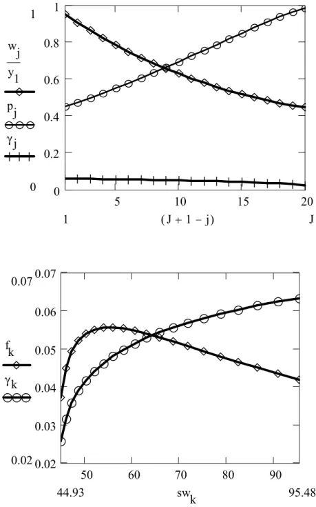
I use two examples to illustrate the wage distribution. In particular, these examples show that the model can generate a hump-shaped density of the wage distribution as the one documented in the literature (e.g., Mortensen, 2002). Since the model is not calibrated to the data, these examples only illustrative. In both examples, I will set J = 20, y1 = 100, c = 0.2yJ and yj =
y1(1 +j∆)1−j for allj, where∆will be determined by the choice ofyJ through the requirement
yJ = y1(1 +J∆)1−J. The two examples differ from each other in ∆ and the distribution of
workers in the labor force. Of course, the equilibrium tightness and wage distribution also differ in the two examples.
Example 5.2. yJ = 98and γj =j0.3.PJj=1j0.3. These imply∆= 5.319×10⁻⁵ andθ= 0.819.
In this example, the difference between the highest and the lowest productivity is small, and the distribution of workers’ productivity in the labor force is a decreasing function. Figure 1 depicts the equilibrium in this example. In the upper panel, the variable on the horizontal axis is an increasing function of productivity. This panel shows that the employment probability is an increasing function of productivity, as the theory predicts. Also, because the productivity differential is small, the wage rate is a decreasing function of productivity.
The magnitude of this reverse wage differential is worth noting: Although the lowest produc-tivity is only 2% lower than the highest producproduc-tivity, the wage of the least productive workers is twice as much as the wage of the most productive workers. Despite this large reverse wage dif-ferential, high-productivity workers are rewarded properly as they receive higher expected wage. This is made possible by a positive differential in the employment probability that outweighs the reverse wage differential.
In Figure 1, I depict the wage density and the distributional density of workers’ productivity. The wage density is hump-shaped. Because the wage rate is a decreasing function of productivity
in this example, the shape of the wage density implies that more workers with medium productiv-ity are employed than workers with either very high-productivproductiv-ity or very low-productivproductiv-ity. There are very few low-wage workers in the equilibrium because these workers are high-productivity workers who are a small fraction of the labor force. There are also very few high-wage workers because these workers are low-productivity workers, who have a very low ranking and hence a very low employment probability.
The shape of the wage density sharply contrasts with the distribution of workers in the labor force, γ. In the lower panel of Figure 1, the plot of γ is the hypothetical density of wages when all workers of each type are employed. In contrast to the humped shape of the actual density, this hypothetical density is increasing. For any wage level, if the actual density exceeds the hypothetical density, the workers at that wage are employed at a rate higher than the average employment rate; if the actual density falls below the hypothetical density, the workers at that wage are employed at a rate lower than the average employment rate. Thus, in this example, low-wage workers are employed at a rate higher than the average rate while high-wage workers are employed at a rate lower than the average rate.
In the above example, the hump-shaped wage density comes with a reverse wage differential. However, this is not an inevitable prediction of the model, as the following example shows.
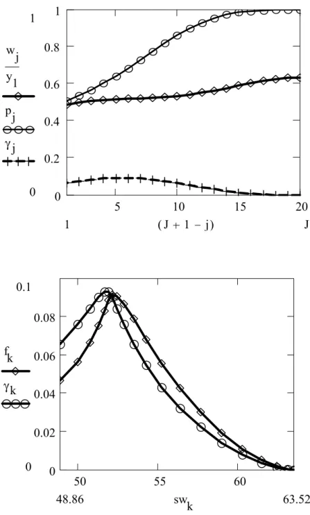
Example 5.3. yJ = 50 and γj = [j(J+ 11−j)]4.PJj=1[j(J + 11−j)]4. These imply ∆ =
1.858×10⁻³ and θ= 0.696.
In contrast to Example 5.2, this example has a much larger difference between the highest and the lowest productivity. As a result, the wage rate is an increasing function of productivity, as depicted in the upper panel of Figure 2. Also, the distribution of workers in the labor force has a single peak at an intermediate level of productivity, rather than being a decreasing function of productivity. Notice that the wage differential is small, in contrast with the large difference in productivity. The large difference in productivity induces a large difference in the employment
probability, and hence in the expected wage. 1 0 wj y1 pj γj J 1 (J 1 j) 5 10 15 20 0 0.2 0.4 0.6 0.8 1 0.07 0.02 fk γk 95.48 44.93 swk 50 60 70 80 90 0.02 0.03 0.04 0.05 0.06 0.07
Figure 1. The equilibrium and the wage density in Example 1
j: worker’s type, with a lowerj corresponding to higher productivity; wj
y1: wage of typej workers, normalized byy1;
pj: employment probability of a typejworker;
γj: fraction of typej workers in the labor force;
sw: wages sorted in an ascending order; f: wage density.
1 0 wj y1 pj γj J 1 (J 1 j) 5 10 15 20 0 0.2 0.4 0.6 0.8 1 0.1 0 fk γk 63.52 48.86 swk 50 55 60 0 0.02 0.04 0.06 0.08
Figure 2. The equilibrium and the wage density in Example 2
j: worker’s type, with a lowerj corresponding to higher productivity; wj
y1: wage of typej workers, normalized byy1;
pj: employment probability of a typejworker;
γj: fraction of typej workers in the labor force;
The density of the wage distribution is still hump-shaped, as depicted in the lower panel of Figure 2. The hypothetical wage density when all workers are employed,γ, is also hump-shaped. In comparison with this hypothetical density, the equilibrium wage density peaks at a higher wage and a larger mass is distributed at higher wages. Thus, low-wage workers are employed at a rate lower than the average employment rate while high-wage workers are employed at a rate higher than the average rate. This result reflects the fact that high-wage workers in this example are high-productivity workers who are employed with a higher probability.
6. Conclusion
In this paper I construct a search model of a large labor market in which workers are heterogeneous in productivity and (homogeneous) firms post wages to direct workers’ search. Each firm can rank the applicants and post different wages for different types of workers. Workers cannot coordinate their applications. In the unique (symmetric) equilibrium, high-productivity workers have a higher priority in employment and higher expected wages than low-productivity workers. The equilibrium is socially efficient. However, high-productivity workers receive higher actual wages than low-productivity workers only when the productivity differential is large. When the productivity differential is small, workers of higher productivity are paid lower wages. Moreover, this reverse wage differential increases as the productivity differential decreases and so it is strictly positive even when the productivity differential approaches zero.
These results suggest that actual wages may not be a good indicator of productivity. They also show that wage differentials among similar workers should not always be construed as dis-crimination, as they have often been viewed in the literature. Rather, the difference in workers’ expected payoffs is a more reliable measure of discrimination. For example, when the produc-tivity differential is so small that it appears statistically insignificant to an econometrician (but observable to the employers), the current model implies that the workers with slightly higher productivity obtain lower wage than other workers. Guided by the convention, the econometri-cian would conclude that high-productivity workers are discriminated against. This would be
misleading, because high-productivity workers enjoy a higher ranking and higher expected wage. A natural question is whether the wage differential can persist in the long run. In a dynamic environment, the search model will have exogenous separation between matchedfirms and work-ers. A wage differential will continue to exist in the steady state, but it may not be reversely related to productivity when the productivity differential is small. For the reverse wage diff eren-tial to survive in the steady state, exogenous job separation must be high. Finding out how high a job separation rate is needed is a quantitative exercise.
An extension to a dynamic economy will also generate some interesting predictions on the time path of wages. For example, consider the model with only two types of workers and suppose that the productivity differential between the two is small. Then, employed workers of high productivity are more likely to search on the job than employed workers of low productivity. This implies that high-productivity workers will have a steeper wage path, even though there is no learning-by-doing or human capital accumulation. Analyzing such on-the-job search is difficult in an environment with directed search. The reason is that, when offering a wage, a firm must take into account not only workers’ tradeoffbetween the wage and the current employment probability, but also the tradeoffbetween the current wage and the probability of getting higher wage in the future. Perhaps a quantitative analysis can be conducted.
Appendix
A. Proof of Proposition 4.2
I can assumeaA>0 andaB>0 without loss of generality. To see this, suppose that an allocation
hasaA= 1,aB= 0 and (qiT, qiS, Ri)i=A,B. Then, an alternative allocation (a∗i, qiT∗ , qiS∗ , R∗i)i=A,B
can be constructed as follows: a∗A = a∗B = 1/2, qAT∗ = qBT∗ = qAT, qAS∗ = qBS∗ = qAS, and
RA∗ =R∗B =RA. This alternative allocation is equivalent to the original allocation, except that
it re-labels a half of thefirms in the original group A as groupB.
Let λj be the Lagrangian multiplier of (4.1) in the planner’s maximization problem. Then,
thefirst-order conditions of qiT andqiS are as follows:
λT/y ≥e−(qiT+qiS)+δe−qiT£Ri+ (1−Ri)e−qiS¤, “ = ” if qiT >0, (A.1)
λS/y≥e−(qiT+qiS)−δ¡1−e−qiT¢(1−Ri)e−qiS, “ = ” if qiS >0. (A.2)
The first-order condition ofaA (taking aB= 1−aA into account) is:
0 = δ¡1−e−qAT¢ £R
A+ (1−RA)e−qAS¤−δ¡1−e−qBT¢ £RB+ (1−RB)e−qBS¤ (A.3)
+he−(qBT+qBS)
−e−(qAT+qAS)i
−(qAT −qBT)λT/y−(qAS −qBS)λS/y.
The following features can be easily deduced from the planner’s problem. First, from inspect-ing the objective function, I can infer that the choice Ri = 1 is efficient whenever qiT > 0 and
qiS >0. Second, it is efficient to utilize both types of workers, in the sense thatqAj+qBj >0 for
both j =T, S. To see this, suppose qAS =qBS = 0, to the contrary. Then, (4.1) does not bind
and soλS = 0. Because typeS workers are not assigned to match with anyfirm, the rankingR
is irrelevant for the allocation, and soRi can be set to 1. In this case, (A.2) implies 0≥e−qiT for
i=A, B, which is a contradiction. Similarly, the choicesqAT =qBT = 0 are not efficient.
With the above features, the efficient allocation must be one of the following cases: (i)qiT >0
and qiS >0 for both i=A and B; (ii) qAT >0 and qAS >0 but qBT = 0 < qBS; (iii) qAT > 0
and qAS > 0 but qBT > 0 = qBS; (iv) qAT > 0 = qAS and qBT = 0 < qBS. (All other cases