Neural network ensembles

(1)

Thesis presented in partial fulfilment of the requirements for the degree of Master of Commerce

at the University of Stellenbosch.

Professor Ian Cloete April2004

(2)

Declaration

I, the undersigned, hereby declare that the work contained in this thesis is my own original work and that I have not previously in its entirety or in part submitted it at any university for a degree.

(3)

Abstract

It is possible to improve on the accuracy of a single neural network by using an ensemble of diverse and accurate networks. This thesis explores diversity in ensembles and looks at the underlying theory and mechanisms employed to generate and combine ensemble members. Bagging and boosting are studied in detail and I explain their success in terms of well-known theoreti-cal instruments. An empiritheoreti-cal evaluation of their performance is conducted and I compare them to a single classifier and to each other in terms of accu-racy and diversity.

(4)

Opsomming

Dit is moontlik om op die akkuraatheid van 'n enkele neurale netwerk te ver-beter deur 'n ensemble van diverse en akkurate netwerke te gebruik. Hierdie tesis ondersoek diversiteit in ensembles, asook die meganismes waardeur lede van 'n ensemble geskep en gekombineer kan word. Die algoritmes "bagging" en "boosting" word in diepte bestudeer en hulle sukses word aan die hand van bekende teoretiese instrumente verduidelik. Die prestasie van hierdie twee algoritmes word eksperimenteel gemeet en hulle akkuraatheid en diversiteit word met 'n enkele netwerk vergelyk.

(5)

Acknowledgements

I am indebted to a very long list of people who supported me during this journey. A big thank you goes to:

• Professor Ian Cloete • Jacolette Stemmet

• My family, especially my parents who instilled in me the passion to learn.

• My church cell group and friends for prayer support! • Jehovah Jireh, the Almighty God.

(6)

2.3 Non-pairwise measures . . . . . 2.3.1 Entropy . . . . . . . 2.3.2 Kohavi-Wolpert variance 2.3.3 Interrater agreement . 2.3.4 Difficulty . . . . 2.3.5 Generalized diversity .. 2.3.6 Coincident failure diversity 2.3.7 Fitness . . . .. . 2.3.8 Implementation . 2.4 Summary . . . . . . . . 2 4 4 5 7 8 10 10 11 11 13 14 14 14 15 15 15 16 16 17 17 17 18 19 19 20 21 21 22

(7)

3 Ensemble Methods

3.1 Process of building an ensemble . 3 .1.1 Generate the base classifiers . 3.1.2 Combine the base classifiers 3.2 Select the single best classifier . 3.3 Linear combinations . . . 3.4 Optimal linear combinations . 3.5 Weighted majority . . . . 3.6 Stacking . . . . . . . . 3. 7 Mixture of expert models 3.8 Overproduce and select .

3.8.1 GASEN . . . . 3.8.2 Image classification.

3.8.3 Generating accurate and diverse members 3. 9 Cooperative Modular Neural Networks

3.10 Summary . . . . . . . . . . . . . . . . . . 4 Bagging

4.1 How does it work?

23 24 24 25 27 27 28 28 30 32 33 33 34 34 35 36 38 39 4.2 Bias-variance decomposition . 40 4.3 0.632 bootstrap . 40 4.4 Simple ensemble . . 41 4.5 Empirical results . . 42 4.5.1 Methodology 42 4.5.2 Accuracy . . 43

4.5.3 Why does the accuracy improvement level off? 44

4.5.4 Diversity . 45

4.6 Summary . . . . . . . . . . . . . . . . . . . . . . . . . 58 5 Boosting

5.1 Background 5.2 How does it work?

5.2.1 Boostl .. . 5.2.2 AdaBoost.M1

5.2.3 Training set error for adaptive boosting. 5.2.4 Arc-x4 . . .

5.2.5 LogitBoost .. . 5.2.6 Ensemble size . 5.2. 7 Weak learners . 5.3 Training set noise . .. 5.4 Bias-variance decomposition . 5.5 Empirical results . . 5.5.1 Methodology 5.5.2 Accuracy . . 59 60 61 61 62 63 65 65 66 68 68 69 70 70 71

(8)

5.5.3 Diversity . . . . 5.5.4 Comparison to bagging 5.6 Summary . . . 6 Conclusion A List of symbols B Data sets B.1 Soybean B.2 Breast-cancer B.3 Iris . . . . B.4 Balance-scale B.5 Heart-c B.6 Heart-h . . B.7 Lymph . . . B.8 Mushroom . B. 9 Hepatitis . . B.10 Horse-colic B.ll Labor . . . 71 75 86 87 89 90 90 90 91 91 91 92 92 92 93 93 93

(9)

List of Figures

1.1 Three fundamental reasons why an ensemble is good 3.1 Algorithm for optimal linear combinations

3.2 Algorithm for weighted majority vote . 3.3 Algorithm for ADDEMUP .

4.1 Algorithm for bagging . . 4.2 Bagging: interesting problems .

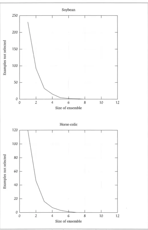
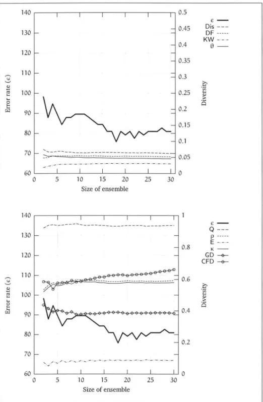
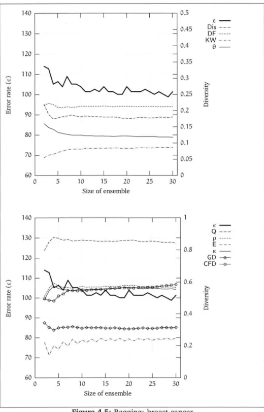
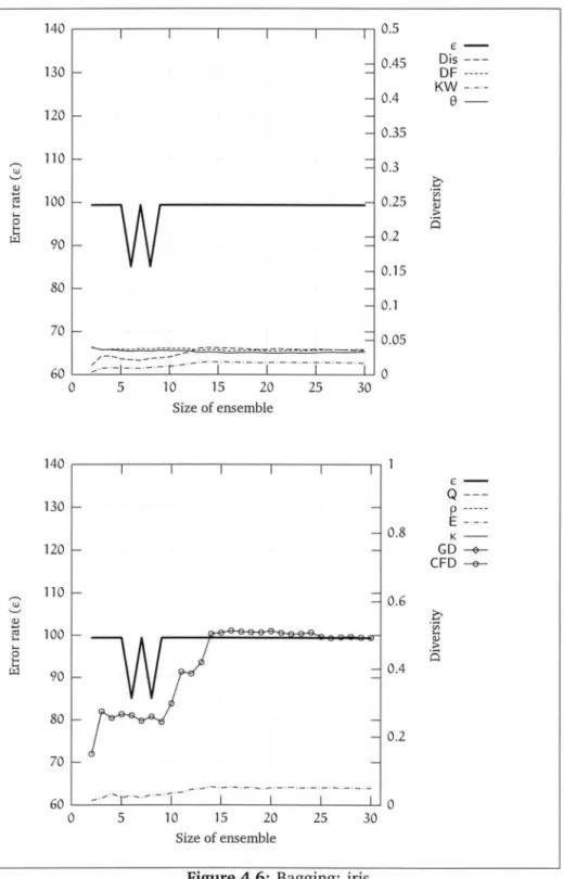
4.3 Number of examples not selected by bagging 4.4 Bagging: soybean . . . . 4.5 Bagging: breast-cancer . 4.6 Bagging: iris . . . . 4. 7 Bagging: balance-scale 4.8 Bagging: heart-c 4.9 Bagging: heart-h . 4.10 Bagging: lymph . . 4.11 Bagging: hepatitis 4.12 Bagging: horse-colic 4.13 Bagging: labor . . . 6 29 31 36 39 42 46 48 49 50 51 52 53 54 55 56 57

5.1 Short history of boosting . 60

5.2 Algorithm for boostl . . . 62

5.3 Algorithm for AdaBoost.Ml 64

5.4 Algorithm for Arc-x4 . . . . 66

5.5 Algorithm for LogitBoost (2 classes) 67

5.6 Boosting: interesting problems . . . 70 5.7 Comparison of AdaBoostMl and Bagging: soybean,

balance-scale . . . . . . . . . . . . . . . . . . . . . . . . . . . . 72 5.8 Comparison of AdaBoostMl and Bagging: hepatitis, horse-colic 73

5.9 AdaBoostMl: soybean . . . 76

5.10 AdaBoostMl: breast-cancer 77

5.11 AdaBoostMl: iris . . . . . . 78

5.12 AdaBoostMl: balance-scale 79

(10)

5.14 AdaBoostM1: heart-h. 5.15 AdaBoostM1: lymph . 5.16 AdaBoostM1: hepatitis 5.17 AdaBoostM1: horse-colic . 5.18 AdaBoostM1: labor .. .. 81 82 83 84 85

(11)

List of Tables

201 Matrix of pairwise Q statistics for an ensemble 0 16

202 Summary of diversity measures 22

401 Example run of bagging 0 0 • 0 40

4o2 Data sets used for empirical analysis 43 403 Error rates for single neural networks 0 44 4.4 Probabilities of an example not being picked by bagging 45

405 Summary of diversity measures 47

501 Example run of boosting 0 0 0 0 61

5o2 Data sets used for empirical analysis 71

5o3 Error rates for single neural networks 0 74 5.4 Summary of diversity measures • 0 0 0 75

(12)

Chapter

1 Introduction

The development of computing and communication technologies has pro-duced a world that lives off information. This is both fascinating and scary. It has become possible for us to google1 _{the internet for background on a} suspicious neighbour, the price of a kite surfing wake board and the last time your friend got a parking ticket. You can check up on your doctor's diagnosis and read about all the side effects of the medicine the pharmacist has given you.

But the most fascinating part is in what you don't know about yourself.

It has become possible for us to search for relationships between see-mingly unconnected pieces of data. Data is the the recorded facts; the innocent events and numbers. Information is the set of patterns and ex-pectations that are waiting to be discovered. Machine learning has made it possible for us to literally read between the lines to extract useful and important information.

A model generated from data by a machine learning algorithm can be regarded as an expert. This expert's quality depends on a lot of factors-the amount and quality of the training data, and whether the machine learning algorithm was suitable for the problem space.

When a wise king makes a decision, he usually takes into account the opinions of several wise people around him rather than relying on his own judgement or that of a single "trusted" advisor. Discussion of different view-points may produce a consensus; otherwise a vote may be called for. It is also important for this wise king to know that his committee of wise peo-ple have different opinions and that they represent the diversity of all the people in his kingdom.

An obvious extension of this would be to also use the opinion of more than one machine learning expert to extract information from data.

(13)

body knows the story of the Mars probe that crashed because of one team of scientists using imperial and another team using decimal units. Could this not have been prevented by a committee of machine learning experts on the probe working together and taking votes for decisions?

This thesis explores the notion of an ensemble of neural network experts. There are several aspects that I specifically want to investigate:

1. How do we build ensembles of neural networks? What is the underly-ing theory and mechanisms?

2. Can we determine if an ensemble of neural networks is more accu-rate than a single network? How do we measure the accuracy of an ensemble?

3. Can we explain the success of some of the well-known ensembling methods?

4. Does diversity in the ensemble members result in more accurate en-sembles? How do we measure the diversity?

This chapter is devoted to introducing the concepts that are specific to the field of neural network ensembles. I explain the thesis layout in sec-tion 1. 7.

(14)

1.1 What is an ensemble?

Suppose we have a supervised learning algorithm. The learning algorithm is given training examples from the training set Z

=

{ (

z

,

-y)} in the problem space 8 (i.e. Z ~ 8) for some function that we are trying to approximate.

The

z

values are vectors of the form (z1, ... , za) consisting of discrete- or real-valued features or attributes. The-y values are drawn from a discrete set of classes lL = {l1 , ... , lm} in the case of classification or from the set of real

numbers in the case of prediction. For the purpose of this section I will only be referring to classification. The training set may be imperfect-it might have some noisy (incorrectly labelled) examples.

The learning algorithm outputs a classifier C after training on the set of training examples Z. This classifier is a hypothesis of the true function.

Given a new example

x

from the problem space, the classifier C will label it with a label l E lL.

An ensemble of classifiers is a set of classifiers whose predictions are combined to produce a single classifier. This resulting classifier is generally more accurate than any of the base classifiers making up the ensemble.

1.2 Why

are ensembles interesting?

An ensemble is usually more accurate than a single classifier. Different clas-sifiers may also implicitly represent different aspects of the training set, while a single classifier cannot represent all useful aspects. An important condition for an ensemble to be more accurate than any of its individual members is that the base classifiers are both accurate (see section 1.3) and

diverse. I discuss the diversity of ensembles in detail in chapter 2.

It is also possible to construct good ensembles that perform better than any of its base classifiers. There are three fundamental reasons (Dietterich (2000)) for this. See figure 1.1 for a depiction.

Statistical A learning algorithm's goal is to construct an approximation of a function f(x). This process can be viewed as a search through the hypothesis space lHI to find the best approximation. This becomes a statistical problem when the number of available training examples are small compared to the size of the hypothesis space. In this case the learning algorithm will find many different approximations (clas-sifiers) of f(x) that have the same accuracy on the training examples.

In the figure there are two curves denoting this situation. The outer curve is the total hypothesis space IHI. The inner curve is the set of classifiers that has the same accuracy on the training examples. If we construct an ensemble out of C1, Cz and C3 we can reduce the risk of

(15)

Computational A learning algorithm usually trains by performing some

kind of local search through the hypothesis space. This search may get stuck in a local maximum. For example, neural networks train by employing back propagation that uses a gradient descent search. Sup-pose we have enough training examples to eliminate the statistical problem. It may still be very difficult to find the best approximation of f(x). If we construct an ensemble by locally searching from different starting points in IHl we have a better chance of not getting stuck in a local maximum.

Representational Our learning algorithm may be unable to approximate

the function f(x)-i.e. f(x) cannot be expressed by any of the hypothe-ses in IHl. If a neural network uses linear activation functions and does not have enough hidden units it may be unable to estimate complex polynomial functions. An ensemble constructed out of the base clas-sifiers C 1, C 2 and C 3 can enlarge the possible space of representable

functions to include f(x).

1.3 What

is

accuracy?

Accuracy is an important aspect of a classifier. For example, we use accuracy as one of the factors to determine whether an ensemble was "better" than a single classifier. Evaluating the accuracy of a classifier is also an integral component of many learning methods. It is therefore important to agree on its definition.

There are three important things to keep in mind when looking at the accuracy of a classifier or ensemble on a limited set of data.

1. How biased is the estimated accuracy? The accuracy of the classifier on the training examples is not a good estimate of its accuracy over unseen examples-the training accuracy is usually too optimistic since the classifier was derived from the training examples.

2. Suppose one classifier does better than another on the limited set of data-does this mean that this classifier is better in general?

3. What is the variance of the estimated accuracy? Even if the classi-fier accuracy is measured over an unbiased set of test examples inde-pendent of the training examples, the measured accuracy can still be different from the true accuracy. This depends on how close the distri-bution of the test set was to that of the function we are trying to learn. A small test set will lead to a greater expected variance.

(16)

Statistical Representational ' ' ,_-?'₀ c1 • f(xl !HI

t

°

Cz

"

I I I I / Computational

Figure 1.1: Three fundamental reasons why an ensemble is good (original figure in Dietterich (2000)).

This leads me to distinguish between sample and true accuracy, or equiv-alently, error. The sample error rate is the fraction of examples misclassi-fied by the classifier C over the sample of data Z:

sample error=

2_

L

b(f(i), C(z)) n

zEZ

where f is the true function that we are trying to approximate and 8 = {

0

1 when f(i) = C(i) when f(i) =J. C(i)

(1.1)

(17)

The true error rate of C is the probability that it will misclassify a single randomly drawn

x

from the input space 8:

true error = Pr ( f ( x) =/:- C( x))

xEEJ

(1.3)

One would usually want to know the true error rate of a classifier; all that we can measure, however, is the sample error rate. Fortunately the sample error rate can be a good estimator of the true error rate, given that we make sure that the test set is independent from the training set and that it contains enough examples for how confident we want the estimation to be.

It might also be worth employing cross-validation. This has a compu-tational impact with processing intensive learning algorithms like neural networks.

1.4 Bias-variance decomposition

The bias-variance decomposition is a useful theoretical tool for evaluating classifiers and ensembles. Several authors (Breiman (1996b), Opitz and Maclin (1999), Kohavi and Wolpert (1996), Witten and Frank (1999)) have used this as part of their proposed theories for the effectiveness of ensem-ble techniques like bagging and boosting. I will be referring back to this decomposition in later chapters.

The total expected error of a particular classifier on a specific target function and training set size has the following three components:

Bias The bias term measures how close the average classifier produced by the learning algorithm will be to the target function. Suppose we have an infinite number of independent training sets for a specific problem space. We can then use these training sets to set up and create an infinite number of classifiers. Take a random test instance and have it processed by all of the classifiers. Let the single ensemble answer be determined by the majority vote (or average if the class is numeric). Even in this ideal situation errors will still occur-no learning scheme is perfect. The error rate will depend on how well suited the machine learning method is to the specific problem. The learning algorithm's bias is defined as the averaged error rate over an infinite number of random test examples. If the bias term is zero we call the classifier unbiased.

The bias term is related to the representational problem in section 1.2.

Variance The variance term measures how much each of the classifier's classifications will vary with respect to each other and is related to the training set in use. The training set is usually finite and seldom

(18)

completely representative of the distribution of the complete problem space. The expected value of this component of the total expected er-ror of the learning algorithm over all the possible training sets is the variance.

Intrinsic target noise This term is defined as the minimum classification error associated with the Bayes optimal classifier for the problem. It is the lower bound of the expected cost associated with any learning algorithm. I explain the concept of a Bayes optimal classifier in the next section.

The bias-variance composition is also sometimes referred to as the

fun-damental decomposition.

Although this is a very interesting way to look at a specific learning algo-rithm it does have limitations when applying it to real-world problems. We need to know what the distribution is that we are trying to learn to estimate the bias, variance and target noise. This is of course unavailable for most real-world problems. Opitz and Maclin (1999) suggested holding out some of the data for this, but the training set size is greatly reduced if you want to get good estimates of the bias, variance and target noise.

1. 5 Bayes optimal classifier

If is often interesting to compare our ensemble to the best hypothesis from the possible hypothesis space IHI, given the set of training examples Z. One way to explain what is meant by the "best" hypothesis is to say that we are searching for the most probable hypothesis, given the training data and any other initial knowledge that we know of the prior probabilities of the hypotheses in IHI. The Bayes theorem provides a direct method for calcula-ting such probabilities-calculate the probability of a hypothesis based on its prior probability, the probability of observing some data given the hypo-thesis and the observed data itself.

Bayes theorem is defined as

( I ) _ Pr(Zih) Pr(h)

Pr hZ - Pr(Z) (1.4)

with the following definitions:

1. Pr(h) is the initial probability that a hypothesis his true, before look-ing at the trainlook-ing data. Pr(h) is usually referred to as the prior

pro-bability of h and will include any background knowledge that may

be available about the chance of h being the correct hypothesis. If

no background knowledge is available, simply assign the same prior probability to every possible h.

(19)

2. Pr(Z) is the prior probability that Z will be observed; given no know-ledge about which hypothesis is selected.

3. Pr(Zih) gives the probability that Z will be observed given the fact that hypothesis h holds.

Pr(hiZ) is the posterior probability of h-it is the confidence that h holds after training with the training examples Z. Pr(hiZ) increases with Pr(h)

and Pr(Zih). Pr(hiZ) decreases as Pr(Z) increases, because when there is a greater chance that Z will be observed independently of h, it also means that Z provides less "evidence" in support of h.

We are interested in finding the best or most probable hypothesis h E IHI,

given the set of training examples Z. Such a maximally probable hypothesis is called a maximum a posteriori (MAP) hypothesis. It is possible to de-termine the MAP hypotheses by using the Bayes theorem to calculate the posterior probability for each candidate hypothesis h E IHI. The MAP hypo-thesis hMAP can be defined as

hMAP = argmaxPr(hiZ) hEIHI Pr(Zih) Pr(h) argmax ( ) hEIHI Pr Z argmaxPr(Zih) Pr(h) hEIHI (1.5)

This far we have been trying to answer the question ''what is the most

probable hypothesis given the training data?" We are actually more interes-ted in what is the most probable classification of a new instance given the training data. This question can be answered by feeding the new instance into the MAP hypothesis, but it is possible to do better.

Consider a hypothesis space containing three hypotheses, h1, h2 and

h₃(example taken from Mitchell (1996)). Let the posterior probabilities of these hypotheses be 0.4, 0.3 and 0.3. This means that h1 is the MAP

hypothesis (highest posterior probability). Take a new instance x and sup-pose h 1 classifies it positively and h2 and h3 classify it negatively. Taking all hypotheses into account, the probability that xis positive is 0.4 and the possibility that it is negative is 0.3

+

0.3

=

0.6. The most probable (nega-tive) classification in this case is not the classification generated by the MAP hypothesis.

Generally the most probable classification of a new instance is the com-bined predictions of all the hypotheses, weighted by their posterior proba-bilities. Take an example

z

E Z that can be labelled by a class label lk E lL.

The probability Pr(lkiZ) that the correct classification for

z

is lk is

(20)

The optimal classification of

z

is the labellk for which Pr(lkiZ) is maxi-mum. This is the Bayes optimal classification:

argmax

L

Pr(lklhd Pr(hi.IZ)

lk ElL h;_ ElHI

(1.7)

No other classification method using the same hypothesis space and same prior knowledge can outperform this method on average. This method maximizes the probability that the new instance is classified correctly; given the set of training examples, the hypothesis space lHI and any known prior probabilities.

1.6 Design and implementation

The object oriented design and analysis process was used for the software developed. This included the normal stages:

• Requirements and initial analysis (setting up a problem statement and deducing the candidate objects, use cases and risks).

• Analysis • Design

• Implementation

The process was adjusted slightly to fit my needs better-! used a more

iterative version (similar to the Extreme Programming model).

1.6.1 Implementation

Implementation took place during several phases. I started out with a C++ neural network implementation and added the bagging ensemble method. During this time we decided to rather use Java. This had the pleasant re-sult of us being able to run our programs on any platform without having to port code. I reused most of the bagging code and built a prototype neu-ral network environment in Java. At this stage I was introduced to the WEKA (Waikato Environment for Knowledge Analysis) environment-a sys-tem developed by the Machine Learning group at the University of Waikato in New Zealand.

WEKA is a comprehensive toolkit for machine learning and data min-ing. Many learning algorithms have already been implemented within an object oriented Java framework. Regression, association rules and cluster-ing algorithms have also been implemented. It includes a variety of tools for transforming and preprocessing datasets. It makes it easy for one to feed a dataset into a learning scheme, and to analyse the resulting classifier and

(21)

its performance. It is enough to say that it is a comprehensive and powerful environment to conduct experiments within.

Rather than to build my own framework, I decided to reuse the exist-ing functionality within WEKA, and to extend it where necessary. WEKA is an open source project and is distributed under the GNU general pu-blic license. This made it easy for me to extend WEKA. The licensing does have implications-if I were to sell my software I would have to provide the sources.

1.6.2 Tools

I employed a number of development tools during the course of this study.

Eclipse (http:/ jwww.eclipse.org) is an open source integrated development environment for Java (among others). It is used as the basis upon which tools like IBM's Websphere Studio for Application Development (WSAD) are built. I used it to develop, debug and distribute my ex-tended WEKA application.

Ant is a general purpose Java build system. It is similar to the GNU make

tool, but much more powerful. I used it to package and deploy my WEKA application. It is available from the Apache Software Founda-tion (http:/ /jakarta.apache.org).

CVS is used for software configuration control and is an acronym for the

Concurrent Versions System (available from http:/ jwww.cvshome.org). It was used for versioning of the software that was developed, as well as for the source files of this thesis.

Bash I wrote quite a lot of bash scripts (part of the Linux operating sys-tem) to automate some of the more mundane tasks-e.g. running sequences of experiments with different numbers of base classifiers in the ensembles.

Log4J is a logging framework for Java available from the Apache Software Foundation (http:/ /jakarta.apache.org). WEKA did not use a proper logging framework and I have started to retrofit it with Log4J.

Linux was used as the operating system on most of the machines that I developed and deployed the WEKA package.

1. 7 Thesis layout

I have attempted to arrange the material in this thesis to create a natural flow of ideas from the beginning to the end. The ideas introduced in this

(22)

In chapter 2 I present a list of diversity measures that can be used to measure diversity (or similarity) in an ensemble of classifiers. Chapter 3 describes the underlying theory of ensemble methods and takes a look at some of the interesting methods that are available.

Bagging (chapter 4) and boosting (chapter 5) are two very well-known ensemble methods. They are described in detail, and I explain the different variations that are available. I test both methods on 11 data sets and present my empirical results-with specific reference to the diversity measures in chapter 2.

Chapter 6 concludes the thesis.

All the symbols used in the thesis are explained in Appendix A. The 11 data sets used for experiments are described in Appendix B.

(23)

Chapter 2 Diversity In Ensembles

An ensemble of classifiers are combined in the hope that the combina-tion will be more accurate than a carefully constructed individual classifier. Chapter 3 will introduce a list of methods available for combining individual classifiers. Most of these methods have been shown to be very successful in improving on the accuracy of the individual base classifiers.

It only makes sense to combine classifiers that make their mistakes on different parts of the input space. A good example would be to take a com-mittee of experts serving as consultants to the CEO of a company. If the committee members were to agree on every question asked of them the company would be better off by having just the best qualified expert in their service-and they would be saving a lot of money! Instead, if the experts were to have different opinions the CEO will be in a much better position to make balanced decisions.

The success of the combining methods introduced in chapter 3 is that, at least intuitively, they build an ensemble of diverse classifiers. Bagging generates data sets for each of the ensemble members by randomly selecting examples from the training set resulting in data sets that are related, but with random differences. There is no specific measure of diversity in this process, but it is assumed that the differences between the generated data sets are a key factor to the success of the bagging algorithm.

Quantifying this diversity is a first step towards trying to link diversity to the ensemble accuracy. The anticipation is also that diversity measures will help us in designing the members of the ensemble and the combination method.

In this chapter I present a list of diversity measures that may be used for measuring diversity in ensembles. There are four pairwise measures

(24)

2.1 Definitions

Let lE = {C 1, Cz, ... , Cn} be an ensemble of n classifiers that classifies exam-ples from the input space 8 that has a attributes. Define lL = {l1, l2, ... , lm} to be a set of m class labels. Let x E 8 be a vector with a attributes.

All the measures in this chapter are discussed in terms of correct I

in-correct decisions-the oracle output. The output Ct(x) is 1 if xis correctly classified by C;_ and 0 if C;_ is wrong. This is an oracle output because it

assumes that the correct class label of xis known.

Every measure can either be described as a diversity or similarity mea-sure. The value of a diversity measure will increase if there is more diver-sity in an ensemble. A similarity measure's value will decrease with more diversity-it is the inverse of a diversity measure. I will categorize each of the measures as either a diversity or a similarity measure.

2.2 Pairwise measures

It is possible to derive many possible measures of the connection between

two classifiers from statistics, but it is less clear when there are three or more classifiers. In this section we look at four pairwise measures and a

way to find the averaged measure over all the classifiers.

2.2.1

Q

Statistics

Let Z = {z1, z2, ... , ZN} be the labelled set of training examples with each

example Zj E 8. C;_ either correctly or incorrectly classifies every

zi.

Let us represent this output of C;_ as the binary vector 1];. = (-y₁,;., -y₂,;_, ... , 'YN,;,),

i

=

1, ... , n, where 'Yi.i.

=

1 if C;, correctly classifies Zj and 'Yi.i.

=

0 if C;, incorrectly classifies Zj.

Yule's Q Statistic (Yule (1900), Kuncheva and Whitaker (2003)) for two classifiers C;, and Ck is defined as

N11NOO- N01N10

Qi.,k = N11NOO

+

N01N10 (2.1)

where

N 11 is the number of examples Zj for which 'Yi.i.

=

1 and 'Yi.k

=

1, N 10 is the number of examples Zj for which 'Yi.i. = 1 and 'Yi.k = 0, N°1 is the number of examples

zi

for which 'Yi.i.

=

0 and 'Yi.k

=

1 and N°0 is the number of examples Zj for which 'Yi.i.

=

0 and 'Yi.k

=

0.

N 11 can also be seen as the number of examples correctly classified by both classifiers, N 10 _{as the number of examples correctly classified by C;,} and incorrectly classified by C k et cetera.

(25)

Q has its maximum value of 1 when N °1 N 10 = 0-the classifiers correctly classify the same examples. If both classifiers always make their mistakes on different examples then N 11 N °0 = 0 and Q = -1. Classifiers that are similar will result in higher (positive) values of Q. Q is a measure of similarity.

2.2.2 Correlation coefficient

The correlation coefficient p between two classifiers C;_ and C k is

(2.3)

Q and p will always have the same sign and Kuncheva and Whitaker (2003)

proved that I

P

I :::;

I

Q

J.

- 1:::; p:::; l. (2.4)

p is also a measure of similarity and more diverse classifiers will result in smaller negative values of p.

2.2.3 Disagreement

The disagreement measure (Skalak (1996), Kuncheva and Whitaker (2003))

is the proportion of examples that only one classifier correctly classifies out of the total number of examples. Note that the total number of examples N =Noo+N01 + N1o+Nll.

N10 + N01

Disi.,k = N for two classifiers C;_ and Ck (2.5)

Dis is a true measure of diversity as it will have higher (positive) values when the classifiers make their mistakes on different examples. Dis will have its maximum value of 1 when N 10 + N°1 = Nand N11 ₊N°0 = ₀

-when there are no examples that both classifiers classify correctly and no examples that both classifiers make mistakes on. Similarly Dis will have its minimum value of 0 when N 11 + N °0 _{= N}_.

0 :::;

Dis:::; 1 (2.6)

2.2.4 Double-fault

The double-fault measure is the proportion of examples that both classifiers

C;_ and Ck make mistakes on out of the total number of examples (Giacinto and Roli (2000), Kuncheva and Whitaker (2003)).

Noo

(26)

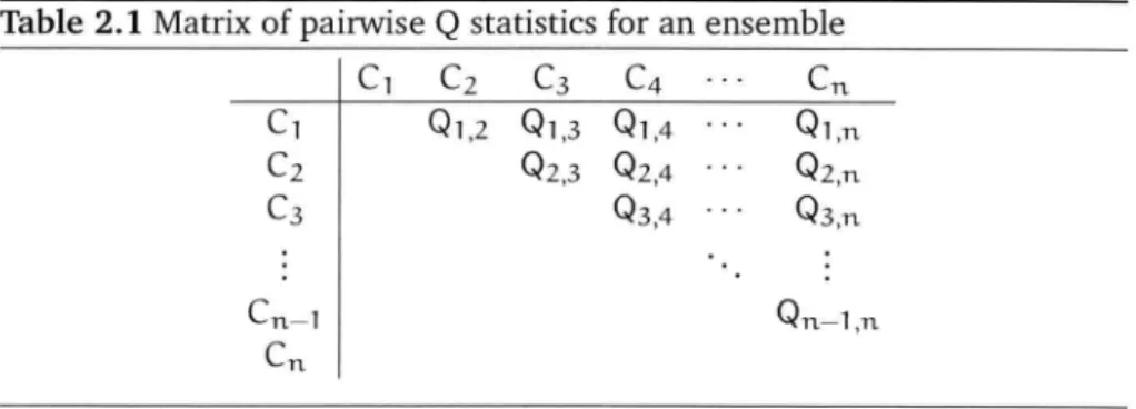
Table 2.1 Matrix of pairwise Q statistics for an ensemble cl 01,2 01,3 01,4 Ol,n C2 02,3 02,4 02,n

c 3 03,4 0 3,n

On-l,n

DF is a measure of similarity as it will have its highest value of 1 when both classifiers misclassify all examples (N°0

_{= N)}

_{. Then we can say}

0 ::; DF ::; 1 (2.8)

2.2.5 Pairwise measures for an ensemble

We would like to use the pairwise measures for an ensemble of more than two classifiers. If one were to calculate all the Q Statistics between all pairs of classifiers Ci and C k in lE the results can be presented in a matrix (see table 2.1). The Q Statistics measure is symmetrical and we only have to compute half of the matrix to be able to get an averaged measure. An ave-raged measure can then be computed for an ensemble of n classifiers as shown in equation 2.9.

2 n-1 n

Oavg = n(n _ ₁)

L L

Oi,k i=l k=i.+ 1

(2.9) This method can be used to calculate all the averaged pairwise diversity measures.

2.2.6 Implementation

I implemented all the pairwise measures in the WEKA system. WEKA al-ready had an Evaluation class that calculates all kinds of statistics on a classifier after it has been trained. It was logical that the diversity mea-sures should also be calculated as part of the ensemble classifier evaluation process.

The diversity measures can only be used on ensemble classifiers like

Bagging and AdaBoost.M1 (package weka.classifiers.meta in WEKA). Since the diversity measures operate on the ensemble's base classifiers I cre-ated an interface that all meta (ensemble) classifiers that want their base classifiers to be evaluated for diversity must implement. The Evaluation

(27)

class always checks if a classifier implements this interface before attempt-ing to calculate the diversity measures on its base classifiers.

2.3 Non-pairwise measures

2.3.1 Entropy

Take an example zi E Z from the input space 8. An ensemble of classifiers has the highest diversity for this Zj when half of the classifiers ( l n/2 J) in the ensemble correctly classify zi and the other half ( n - l n/2 J) misclassify zi.

Define l( Zj) to be the number of ensemble base classifiers ( C;_) that correctly classifies a Zj. The Entropy Measure E (Kuncheva and Whitaker

(2003)) is defined in equation 2.10.

E =

2_

£.

min{l(zj), n - l(zj)}

N . n - ln/2J

J=l

(2.10)

E has its highest diversity value of 1 when l(zj) = ln/2J, Vj. E has its lowest value of 0 when l(zj) =nor l(zj) = 0, Vj.

(2.11) E is a measure of diversity.

2.3.2 Kohavi-Wolpert variance

Kohavi and Wolpert (1996) defined the variance of the predicted class label -y for x E 8 across training sets for a specific classifier as

(2.12)

Remember that l;_ E lL was defined as one of m possible class labels for every x in section 2.1. For the oracle output we are only interested in two possible class labels: lL = {0, 1}. Kuncheva and Whitaker (2003) used this idea in the following way: look at the variance of the predicted class label -y for the given training set using the base classifiers from the ensemble lE.

Kohavi and Wolpert (1996) estimated Pr(-y = l;_)fx) as an average over the different data sets. For the oracle output we can estimate Pr(-y = Ofx)

and Pr(-y = 1fx) for the training set over all the base classifiers C;_, i =

1, 2, ... , n as

JJ(-y = 1fx) = l(x) and JJ(-y = Ofx) = n - l(x) ₍₂_.₁₃₎

(28)

If you substitute equation 2.13 into equation 2.12 you get variancex

=

~

(

1 - 15(-y

=

1lx)2- 15(-y

=

Olx)2)

~ (₁_ l(x)2 _ (n - l(xlf )

2 n2 _n2

l(x)(n - l(x))

n2 (2.14)

Take the average of equation 2.14 over all the examples zi E Z, and define the Kohavi-Wolpert variance (Kuncheva and Whitaker (2003)) to be

(2.15)

KW has its smallest diversity value of 0 when l(zj)

=

0 or l(zj)

=

n, Vj. This will happen if all the classifiers classified all the Zj correctly or were wrong for all the examples. KW will have its largest value of 1/4 when l(zj) = ln/2J,Vj.

0

<

_-

KW

<

_-

~

₄

KW is a measure of diversity.

2.3.3 Interrater agreement

(2.16)

This measure is derived from the measure of interrater reliability, K, which

is used to determine the level of agreement of raters assessing subjects. Kuncheva and Whitaker (2003) adjusted this measure to make it usable in our context-classifiers Craters) and training examples (subjects).

Let

p

be the average base classifier accuracy.

Then we can define

K 1 N 1 n

p

= N .[_

n

.[_

1Ji,i j=l i=l 1 _ ~ .L~

1

l(zi)(n - l(zj)) N(n - 1)p(1- p) 1- n KW ( n - 1 )p ( 1 - p) (2.17) (2.18) (2.19) The measure of interrater agreement is a measure of similarity since larger values of K will occur when the ensemble base classifiers are more

(29)

similar. Diverse base classifiers will result in negative values of K. The value

of K is dependent on

p

and n. When

p

----1 0 or

p

----1 1 it will result in a very

large factor for KW-resulting in a possible large negative (diverse) value of K.

2.3.4 Difficulty

Define X to be a discrete random variable taking values in {0/n, 1 /n, ... , 1 }. The possible values of X describe the proportion of classifiers from Ci E lE correctly classifying a random

x

E 8. In other words-X tells us how difficult it was for the ensemble to classify a random

x.

The measure of difficulty is based on the distribution of X.

Kuncheva and Whitaker (2003) suggested capturing this distribution shape by using the variance of X, er~, as the measure of difficulty 8.

We know that er~ E[X2] - (E[X])2 f.Lxz - (f.lx)2 .[_ xPr(xiX) xEX (2.20) (2.21)

We estimate Pr(xiX) (equation 2.21) for all the training examples Zj E 7l by building a histogram showing how many examples did 0/n, 1 /n, ... , n/n classifiers correctly classify-define h(x) to be the number of examples cor-rectly classified by x E X classifiers. Then

P(xiX) = h(x) N from which we can calculate f.lx and f.Lxz.

(2.22)

Higher values of 8 will mean a less diverse classifier team. The ideal (most diverse) ensemble will have 8 = 0. This implies that 8 is a measure of

similarity.

2.3.5 Generalized diversity

Krzanowski and Partridge (1997) proposed this measure as part of an article about diversity in software. They did a study on how different and diverse versions of mission-critical software systems (for example air craft guidance systems and nuclear reactor protection systems) could prevent software fai-lure through inevitable errors.

Let Y be a discrete random variable taking values in {0/n, 1 /n, ... , 1 }. The possible values of Y describe the proportion of classifiers from Ci E lE incorrectly classifying a random

x

E 8 (Y is the inverse of X introduced in

(30)

section 2.3.4). Define p(i) to be the probability that i classifiers randomly picked from lE misclassify a random

x

.

Krzanowski and Partridge (1997) suggested that maximum diversity in a software system occurs when one randomly chosen part of the system failing results in another randomly chosen part not failing. In our case this would translate into maximum diversity when one randomly chosen Ci. E lE fails and another C k E lE correctly classifies a random example. The probability of both classifiers failing in this case is then p(2) = 0. Minimum diversity will be when failure of one classifier is always accompanied by failure of the other classifier. Then p(2) = p(1 ).

Krzanowski and Partridge (1997) proved that p(1) =

f.

~Pr

(

Y=i

/

n

)

n i.=l n i(i- 1) p(2) =

~

n(n _ ₁) Pr(Y = i/n) l=l (2.23) (2.24)

We can estimate Pr(Y = i/n) similar to equation 2.22. Krzanowski and Partridge (1997) defined the generalized diversity measure as

GD = 1- p(l)

p(l) (2.25)

GD will indicate maximum diversity of 1 when p(2) diversity occurs when GD = 0 and p(2) = p(1 ).

0. Minimum

0

:S

GD

:S

1 (2.26)

GD is a measure of diversity.

2.3.6 Coincident

failure

diversity

Krzanowski and Partridge (1997) also proposed a modification to general-ized diversity-coincident failure diversity. CFD will have a minimum value of 0 (no diversity) when all classifiers are always correct or when all clas-sifiers are simultaneously correct or wrong. CFD will have its maximum value of 1 (very diverse ensemble) when at most one classifier will fail on any random chosen example.

{

0, Pr(Y = 0/n) = 1

CFD = l-Pr(L o;n) Li.=l

n~_:_:~

Pr(Y = i/n), Pr(Y = 0/n) < 1 (2·27) Once again we can estimate Pr(Y = i/n) similar to equation 2.22.

0

:S

CFD

:S

1 (2.28)

(31)

2.3. 7 Fitness

Opitz and Shavlik (1996) used thefitness measure as part of their ADDEMUP

algorithm to help prune their generated ensembles of the least fittest base

classifiers. They combined the base classifiers using a simple weighted sum of the base classifier outputs:

n n

CJ

=

L

Wi · (i With

L

Wi

=

1

i=l i=l

They then define a "diversity" measure di for classifier Ci N

di = .L_rci(zj)-&(zjlf

j=l

The fitness measure F for classifier i is defined as Accuracyi

+

.\di

(1 - Et)+ Adi

(2.29)

(2.30)

with Ei the error rate of classifier i and .\ a trade-off between accuracy and

diversity. Diverse and accurate ensemble members will have a greater value

of Fi. Furthermore Fi ~ 0. This means that F is a measure of diversity. We can determine the average fitness of the ensemble by averaging Fi

over all the ensemble classifiers.

1 n

F = -

L

Fi

n (2.31)

i=l

2.3.8 Implementation

I implemented all the non-pairwise measures in the WEKA system-similar to the pairwise measures. If a classifier implements the MetaClassifier interface its non-pairwise measures will be computed and displayed as part of the normal evaluation process.

(32)

Table 2.2 Summary of diversity measures. An up-arrow Cf) specifies that it

is a measure of diversity. A down-arrow (1) specifies that it is a measure of similarity.

Pairwise

Q Statistics Q

_l

- 1:S: Q:S: 1

Correlation coefficient p

_l

-1 :S:p:S: 1

Disagreement Dis

_T

0 :::; Dis :::; 1

Double-fault DF

_l

0 :S: DF :S: 1 Non-pairwise Entropy E

_T

0 :S: E:S: 1 Kohavi-Wolpert variance KW

_T

0 :S: KW :S: 1/4 Interrater agreement K

_l

Difficulty

e

_l

8 ?:0 Generalized diversity GD

_T

0 :S: GD :S: 1

Coincident failure diversity CFD

_T

0 :::; CFD :::; 1

Fitness F

_T

F?:O

2.4 Summary

Table 2.2 summarizes the eleven different measures of diversity introduced

in this chapter. In the following chapters we will use these measures to de-termine if there is some kind of relationship between ensemble accuracy and diversity and if there are specific ensemble methods that are more suitable

for generating diverse ensembles.

One has to be careful in using these measures-they should be used

in conjunction with the normal accuracy measures. The fitness measure

(section 2.3. 7) is a good example of how I think one should be using the

(33)

Chapter 3 Ensemble Methods

An ensemble of classifiers is a set of classifiers whose predictions (or classifi-cations) are combined to produce a single superior classifier. The ensemble is usually more accurate than any single base classifier and may be able to better represent the classification problem.

There is a myriad of ensemble methods available today and they all have the same basic steps that take place as part of the ensemble process:

1. Generate the members of the ensemble. 2. Combine the members' predictions.

I explain this general process in section 3.1 and describe the basic techniques that are used in most methods.

The last part of the chapter (sections 3.2 to 3.9) introduces some well-known ensemble methods.

(34)

3.1 Process

of building an ensemble

This section outlines the high-level ideas behind many of the ensemble methods in use.

3.1.1 Generate the base classifiers

Training examples

This is a common method for generating multiple base classifiers and is effective for unstable learning algorithms like neural networks and decision trees. The learning algorithm is run several times with a different set of examples based in some way on the original set of training examples:

1. Divide the training set into a number of disjoint subsets. Construct the base classifiers by running the learning algorithm on sets formed by leaving out a different disjoint subset for every iteration. This is similar to the process of cross-validation and ensembles constructed in this way is sometimes also called cross-validated committees.

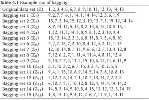
2. Take bootstrap replicates of the training set by drawing random exam-ples from it (with or without replacement). The most famous way of perturbing the training examples in this way must be bagging-it is explained in detail in chapter 4.

3. Add artificial noise to the training examples. This randomness is usu-ally enough for unstable procedures to start their search at a different place in the hypothesis space. One can either add random noise to the training examples or add small amounts of noise to the input at-tributes, but leave the outputs as is. This is also known as jittering.

Input features

In cases where the input features (attributes) are highly redundant one can also manipulate the set of input features available to the learning algorithm.

In cases where the classes are representable by entirely different feature domains the generation of random subsets out of a large feature set also appears to be successful.

Output targets

This general technique works by manipulating the class labels that are given to the learning algorithm. Dietterich and Bakiri (1995) developed a method called error-correcting output coding from this general technique.

(35)

Learning algorithm

An obvious method of generating different base classifiers is to manipulate the learning algorithms. This can be done in any of the following ways:

1. Initialize the learning algorithm with different parameters for every new base classifier. This can include random weights for neural net-works and different parameter choices like the number of hidden nodes and layers. This is useful for injecting randomness into the learning algorithm.

2. Use heterogeneous sets of classifiers built using different learning al-gorithms in the same feature space and using the same training set. Different classifiers are able to express their opinions in different ways.

3.1.2 Combine the base classifiers

Voting

Voting is commonly used with classification and several variations exist: 1. An unanimous vote. The ensemble classifies a new example

x

as l only

if all the base classifiers classified the new example with l.

2. Modified unanimous vote. The ensemble classifies a new example

x

as l if some base classifiers classified the new example as l and no other classifier labelled the new example with another class (rejects it). 3. A majority vote (weighted or unweighted). The ensemble decides that

the new example

x

belongs to class l if more than half of the base classifiers support that

x

belongs to l. This rule is sometimes modified to require a different proportion of classifiers to agree.

4. Threshold plurality. The ensemble decides that

x

belongs to the class l if the number of classifiers that support it is considerably bigger than the number of base classifiers that support any other class.

Fixed rules

The fixed combining rules (Duin (2002)) make use of the fact that the out-puts of the ensemble's base classifiers have a clear definition. It is not just numbers-it may be class labels, distances, probabilities and predictions. Suppose our base classifiers were to predict the probability of an example

x

being in a class l. There are several possible ways to combine these base classifiers into an ensemble.

(36)

1. The product rule is good if the individual base classifiers are indepen-dent. If performs best when the base classifiers are trained on different feature spaces.

The rule also needs noise free and reliable confidence estimates and fails when the estimates are zero or very small.

2. The sum rule is often used with ensembles of predictors. It usually takes the form of an average of the outputs of the base classifiers or a weighted sum.

The rule works well with a collection of similar base classifiers with independent noise behaviour-the errors in the probabilities are ave-raged out by the summation. This rule is equivalent to the product rule when the classifier outputs are similar, but still independent. 3. The maximum rule selects the classifier that is most confident. This

fails when some of the base classifiers are over-trained.

It is difficult to find applications for which this rule works well. 4. The minimum rule selects the classifier that has the least objection

against a classifier; similarly to the maximum rule it is not easy to find applications for this rule.

5. The median rule is similar to the sum rule, but is sometimes more robust.

Combining classifier

Instead of using voting or a fixed rule one can also use the training set and the outputs of the base classifiers to train another classifier to combine the base classifiers into an ensemble. One has to carefully consider how much and what subset of the training set to use for training the combining classifier as it is very easy to over-train the ensemble with this method.

(37)

3.2 Select

the single best classifier

The simplest form of an "ensemble" is simply selecting the single best or most accurate classifier from a set of base classifiers generated in some way.

It is simple to use and easy to understand what is happening. It does how-ever have the problems explained in sections 1.2 and 1.4.

One has to have an independent set of examples for evaluating the set of base classifiers and this set cannot be the same as the test set. If your set of labelled examples is small you might not have enough data to do this properly and you might select an over-trained classifier as the "best"

classifier. This "best" classifier will in general perform worse on unseen data than some of the other generated classifiers.

A variation of this idea is discussed in section 3.8.

3.3 Linear combinations

Ensembles of predictors are often combined using the average or weighted sum of the outputs of the base classifiers. It is simple to construct and, depending on the method used to construct the base classifiers, often out-performs any single best base classifier. The ensemble members can be con-structed in any way. A linear combination of classifiers is a fixed summation rule.

From a neural network perspective linearly combining the outputs of a

number of trained neural networks is similar to setting up a single large neural network in which the trained neural networks are smaller networks operating in parallel. The combination weights are the connection weights of the output layer. For a given example

x

the output of the combined model is the weighted sum of the outputs of the component neural networks.

The general form of the linear combination is

n

E=.L_wici

i=l

where the {wi} is a set of weights that may sum up to one. Using

1 .

w,

=

-,

v

'l.

n

is the common method of averaging the outputs of the ensemble members. Granger and Ramanathan (1984) considered three different approaches to obtaining linear combinations. They found that the best method is not to use the common practise of a weighted sum with the weights adding up to one. One should rather add a constant term to the sum and not constrain

(38)

the weights to add up to unity:

n

lE =wom+

L

wiCi i=l

(3.1)

with m the mean of the outputs of the base classifiers. The weights {wi} are obtained by regression.

Linear combinations mainly work by attacking the statistical problem described in section 1.2.

3.4 Optimal linear combinations

Hash em et al. (1994) also proposed using an "optimal" linear combination of neural networks instead of a single best network. The optimal combina-tion is constructed in a way similar to equation 3.1. Hashem et al. (1994) found that their optimal combination was better than that of the single best trained neural network and that of the simple averaging of the outputs of the base networks.

They set m = 1 and found that the optimal weights {wi} are equal to the ordinary least squares regression coefficients. The weights are not con-strained to sum to unity. This algorithm is shown in figure 3.1.

Hashem et al. (1994) found that the optimal linear combination method performed better on poorly trained neural network base classifiers than on well-trained networks. For well-trained networks the combination weights tended to automatically sum to unity, with the constant term w0

approach-ing 0. This can be explained by the fact that the base networks are close to the approximated function and have little bias. For the poorly trained networks the combination weights did not sum to unity while the constant term was significantly different from 0. In the case of the well-trained net-works the optimal linear combination method operated in a "fine-tuning" role, while for the poorly trained networks it performed a significant model-ling role.

3.5 Weighted majority

The weighted majority algorithm (Littlestone and Warmuth (1992)) is a simple and effective method that can construct an ensemble that is robust in the presence of errors in the data. The algorithm makes predictions by taking a weighted vote among a pool of prediction algorithms and builds the ensemble by altering the weight associated with every base classifier.

First we have to construct and train the set of base classifiers using methods derived from section 3.1.1. These classifiers make varying num-bers of mistakes. The goal of the weighted majority algorithm is not to

(39)

Ensemble generation

Require: A labelled training set Z. Base neural network architectures-may be the same or different.

for i

=

1 to n do

Construct neural network

Ct

according to architecture settings and with random connection weights.

Train this neural network with the whole training set Z. Construct the ensemble

n

lE=wo+L,wiCi i=l

and estimate the combination weights by least squares regression.

Classification procedure

Require: An unseen example

x.

Feed the example into the ensemble.

Figure 3.1: Algorithm for optimal linear combinations

make more mistakes than the best algorithm in the pool, even though it does not have any knowledge about the accuracy of the base classifiers.

The weighted majority algorithm begins by assigning a weight of 1 to every base classifier in the pool and then uses the set of training examples to modify these weights to reflect the accuracy of the base classifiers. Ensemble "learning" then proceeds in a sequence of iterations (see figure 3.2). In every iteration the algorithm takes an example from the set of training examples and feeds it to each of the base classifiers. Each classifier makes a prediction and these predictions are grouped together to enable the master algorithm to make its prediction. If the master algorithm misclassifies an example each base classifier that has misclassified that example has its weight reduced by a factor 0 :::;

f3

:::;

1. This makes it possible for the weighted majority algorithm to accommodate inconsistent training data. The algorithm never completely eliminates a base classifier but only reduces its weight. The weight of a classifier represents the "belief" of the master algorithm in the accuracy of the member.

If the weighted majority algorithm is used with equal weights and

f3

= 0, it is identical to the halving algorithm. If

f3

>

0, weighted majority gradually decreases the influence of base classifiers that make a large number of mis-takes and gives the classifiers that make few mismis-takes high relative weights.

I have described the basic weighted majority algorithm where the pre-dictions of the base classifiers and the ensemble as well as the labels of the examples are required to be binary. Various variants of the algorithm exist that that allow continuous predictions.

(40)

Littlestone and Warmuth (1992) proved that the number of mistakes m

made by weighted majority

klog2 i

+

log₂n

m

<

2

logz 1+13

where k is the minimum number of mistakes made by any base classifier and n is the number of classifiers in the ensemble. This means that the number of mistakes made by weighted majority will never be greater than a constant factor times the number of mistakes made by the best classifier in the ensemble, plus a term that grows logarithmically with the size of the ensemble.

The prediction of the weighted majority vote is based on the weighted

average of the predictions of the ensemble base classifiers. In that way it is similar to linearly combining predictions through a method like optimal linear combinations. Weighted majority works because it attacks the

sta-tistical problem (section 1.2) and reduces the variance of the bias-variance decomposition (section 1.4) of the total expected error.

3.6 Stacking

Stacked generalisation (Wolpert (1992)) can also be used for combining base classifiers (section 3.1.2). Stacking is generally used to combine base classifiers that are not of the same type-an ensemble of decision trees and neural networks, for example. Stacking introduces the notion of a meta learner-replacing the voting or averaging combining mechanisms that one finds in ensemble methods like bagging and boosting. With the meta learner stacking tries to learn how trustworthy each of the base classifiers in the ensemble is. The meta learner is another learning algorithm-for example a neural network-that trains on the outputs of the base classifiers. Some

researchers also suggest using some of the inputs to the base classifiers in conjunction with the base classifiers' outputs; I am of the opinion that this will increase the chances of over-training the ensemble.

The meta learner tries to learn which of the base classifiers are more reliable-and thus how to best combine them. The meta learner has the same of number of inputs or attributes as the number of base classifiers-and these attribute values are simply the predictions of the base classifiers. During classification an instance is first fed into the base classifiers, and each one predicts a value. These predictions are then fed into the meta learner to be combined into a single final prediction.

Unfortunately we can't use the same training examples that have been used to train the base classifiers to also train the meta learner-for the same

(41)

Ensemble generation

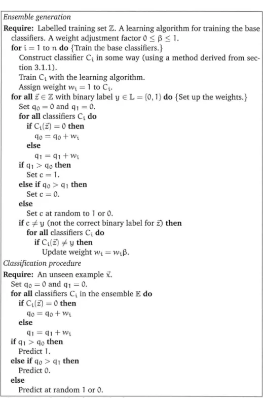
Require: Labelled training set Z. A learning algorithm for training the base classifiers. A weight adjustment factor 0 :::; j3 :::; 1.

for i

=

1 to n do {Train the base classifiers.}

Construct classifier C;_ in some way (using a method derived from sec-tion 3.1.1).

Train C;_ with the learning algorithm. Assign weight w;_

=

1 to C;_.

for all i E Z with binary label11 E L = {0, 1} do {Set up the weights.}

Set q₀= 0 and q₁= 0. for all classifiers C;_ do

if C;_(z)

=

o then Qo = Qo + w;_ else Q1 = Ql + w;_ if Ql > Qo then Set c = 1. else if q0

>

q1 then Set c = 0. else Set c at random to 1 or 0.

if c =I= 11 (not the correct binary label for i) then for all classifiers C;_ do

if C;_(Z) =I= 11 then

Update weight w;_ = w;_j3.

Classification procedure

Require: An unseen example

x.

Set Qo

=

0 and Q1

=

0.

for all classifiers C;_ in the ensemble lE do if C;_(z) = 0 then Qo = Qo + w;_ else Ql = Ql + w;_ if Q1

>

Qo then Predict 1. else if Qo

>

Q1 then Predict 0. else Predict at random 1 or 0.

Figure 3.2: Algorithm for weighted majority vote. Assumes the base classi-fiers does binary classification.

(42)

true error rate. We are trying to use the meta learner to learn the reliability of the base classifiers. If we reuse the training examples we will be too optimistic-some of the base classifiers may be over-trained on the training examples and will receive an incorrect better rating. For this reason we have to have two sets of training examples-one for the base classifiers and another one for training the meta learner. The set used for training the meta classifier must never be used during training of the base classifier. In this way the base classifiers' predictions will be unbiased and the meta learner will be more accurate.

This process does make the training set even smaller. It is possible to incorporate the process of cross-validation in conjunction with stacking to make better use of the available data.

In his paper "The Combining Classifier: to Train or Not to Train", Duin (2002) has some interesting points that relate to stacking. He remarks that if the base classifiers have been trained independently (i.e. using different feature sets or different numbers of epochs) one must look carefully at their outputs. It may be necessary to calibrate or scale the outputs. Duin (2002) also proposed the following strategies for using the training data:

• Use a single training set for both the base classifiers and the meta model. Train the base classifiers carefully to avoid over-fitting. Reuse the training set for training the meta learner.

• Use a single training set for both the base classifiers and the meta model. Train the base classifiers weakly. Reuse the training set for training the meta learner.

• Separate the training examples into two sets. Use one set for training the base classifiers and another set for training the meta learner. Stacking can help us find a solution for the representational problem de-scribed in section 1.2.

3.7 Mixture of expert models

Milidiu et al. (1999) described a system consisting of a mixture of different learning models suitable for time series forecasting. The training examples are partitioned into disjoint sets using a clustering algorithm. Every disjoint set is then used for training a number of different learning models. For every disjoint set a "winning" model is then chosen based upon accuracy on the independent test set. The strength of this method is that it always uses the most appropriate learning algorithm for the specific cluster of training data-reducing the bias (section 1.4).

The MEM system starts by doing a Haar wavelets transform on the train-ing examples. This prepares the training set for the clustering algorithm