Acronyms and Definitions
ASD Analytical spectral devices
AISA Airborne imaging spectrometer for applications
AVIRIS Airborne visible/infrared imaging spectrom
eter sensor
CHRIS PROBA Compact High Resolution Imaging Spectro meter Project for OnBoard Autonomy, Belgian Satellite
DHVIs Derivative hyperspectral vegetation indices
(DHVIs)
DNs Digital numbers
EnMAP Environmental Mapping and Analysis
Program, Genrman’s hyperspectral satellite mission
EO1 Earth Observing1 satellite of NASA
GnyLi A hyperspectral vegetation index involving
5 hyperspectral narrow bands developed by Martin Gnyp Leon, Fei Li, and Georg Bareth et al.
HICO Hyperspectral Imager for Coastal Oceans
sensor, NASA’s Hyperspectral Imager for the Coastal Ocean (HREPHICO)
HBSIs Hyperspectral biomass and structural indices
HNBs Hyperspectral narrow bands
HVIs Hyperspectral vegetation indices (HVIs)
HyspIRI Hyperspectral infrared imager, nextgenera
tion hyperspectral sensor by NASA
MBHVI Multiple band hyperspectral vegetation indices
MNF Minimum noise fraction
NASA National Atmospheric and Space
Administration
9
Hyperspectral Remote Sensing
for Terrestrial Applications
Acronyms and Definitions ...201
9.1 Introduction ... 202
9.2 Hyperspectral Sensors ... 203
Spectroradiometers • Airborne Hyperspectral Remote Sensing • Spaceborne Hyperspectral Data • Unmanned Aerial Vehicles • Multispectral versus Hyperspectral • Hyperspectral Data: 3D Data Cube Visualization and Spectral Data Characterization • Past, Present, and NearFuture Future Spaceborne Hyperspectral Sensors • Data Normalization Hyperspectral Data 9.3 Data Mining and Data Redundancy of Hyperspectral Data ...210
9.4 Hughes’ Phenomenon and the Need for Data Mining ...210
9.5 Methods of Hyperspectral Data Analysis ...212
9.6 Optimal Hyperspectral Narrowbands ...213
9.7 Hyperspectral Vegetation Indices ...213
TwoBand Hyperspectral Vegetation Indices • MultiBand Hyperspectral Vegetation Indices 9.8 The Best Hyperspectral Vegetation Indices and Their Categories ...217
9.9 Whole Spectral Analysis ...219
Spectral Matching Techniques • Continuum Removal through Derivative Hyperspectral Vegetation Indices 9.10 Principal Component Analysis... 220
9.11 Spectral Mixture Analysis of Hyperspectral Data ... 222
9.12 Support Vector Machines ... 223
9.13 Random Forest and Adaboost TreeBased Ensemble Classification and Spectral Band Selection ... 223 9.14 Conclusions... 230 References ... 230 Prasad S. Thenkabail U. S. Geological Survey Pardhasaradhi Teluguntla U. S. Geological Survey and
Bay Area Environmental Research Institute
Murali Krishna Gumma
International Crops Research Institute for the Semi Arid Tropics
Venkateswarlu Dheeravath
United Nations World Food Programme
OHNBs Optimum hyperspectral narrow bands
OMI Ozone Monitoring Instrument onboard Aura
satellite
PCA Principal component analysis
PRISMA Hyperspectral Precursor and Application
Mission or PRecursore IperSpettrale della Missione Applicativa of Italy
SCIAMACHY Scanning Imaging Absorption spectroMeter
for Atmospheric CartograpHY, hyperspec tral sensor onboard European Space Agencies (ESA’s) ENVISAT
SMA Spectral mixture analysis
SMT Spectral matching techniques
SVM Support vector machines
TBHVIs Twoband hyperspectral vegetation indices
VNIR Visible and nearinfrared (VNIR)
WSA Whole spectral analysis
9.1 Introduction
Remote sensing data are considered hyperspectral when the data are gathered from numerous wavebands, contiguously over an entire range of the spectrum (e.g., 400–2500 nm). Goetz (1992) defines hyperspectral remote sensing as “The acquisition of images in hundreds of registered, contiguous spectral bands such that for each picture element of an image it is possible to derive a complete reflectance spectrum.” However, Jensen (2004) defines hyperspectral remote sensing as “The simulta neous acquisition of images in many relatively narrow, con tiguous and/or non contiguous spectral bands throughout the ultraviolet, visible, and infrared portions of the electromagnetic spectrum.”
Overall, the three key factors in considering data to be hyper spectral are the following:
1. Contiguity in data collection: Data are collected contigu
ously over a spectral range (e.g., wavebands spread across 400–2500 nm).
2. Number of wavebands: The number of wavebands by itself
does not make the data hyperspectral. For example, if there are numerous narrowbands in 400–700 nm wave lengths, but have only a few broadbands in 701–2500 nm, the data cannot be considered hyperspectral. However, even relatively broad bands of width, say, for example, 30 nm bandwidths spread equally across 400–2500 nm, for a total of ~70 bands, are considered hyperspectral due to contiguity.
3. Bandwidths: Often, hyperspectral data are collected in
very narrow bandwidths of ~1 to ~10 nm, contiguously
over the entire spectral range (e.g., 400–2500 nm). Such narrow bandwidths are required to get hyperspectral sig natures. But one can have a combination of narrowbands and broadbands spread across the spectrum and meet the criterion for hyperspectral remote sensing.
In summary
Remote sensing data are called hyperspectral when the data are collected contiguously over a spectral range, pref erably in narrow bandwidths and in reasonably high num ber of bands.
Such a definition will meet many requirements and expec tations of hyperspectral data.
Hyperspectral remote sensing is also referred to as imag ing spectroscopy since data for each pixel are acquired in numerous contiguous wavebands resulting in (1) 3d image cube and (2) hyperspectral signatures. The various forms and characteristics of hyperspectral data (imaging spec troscopy) are illustrated in Figures 9.1 through 9.7. The dis tinction between hyperspectral and multispectral is based on the narrowness and contiguous nature of the measure ments, not the “number of bands” (Qi et al., 2012).
The overarching goal of this chapter is to provide an intro duction to hyperspectral remote sensing, its characteristics, data mining approaches, and methods of analysis for terrestrial appli cation. First, hyperspectral sensors from various platforms are
(a) (c) 0.6 Beech Poplar Soil 0.4 Refle ct an ce (–) 0.2 0 500 1000 1500 Wavelength (nm) 2000 2500 (b)
Figure 9.1 Tree spectra. Analytical Spectral Devices (ASD) FieldSpec JR spectroradiometer. Hyperspectral shapebased unmixing to improve intra and interclass variabilities for forest and agro ecosystem monitor ing. A detail of a 30by30 m image pixel of the virtual forest consisting of two species with a different structure, with 10% of the trees removed to include gaps in the canopy (a). An example of a virtual tree for the two species, used to build up the forest, is shown in (b), while the spec tral variability of the two species and the soil is given as well (c). (From Tits, L. et al., ISPRS J. Photogramm. Remote Sens., 74, 163, 2012.)
noted. Second, data mining to overcome data redundancy is enu merated. Third, concept of Hughes’s phenomenon and the need to overcome it are highlighted. Fourth, hyperspectral data analysis methods are presented and discussed. Methods section includes approaches to optimal band selection, deriving hyperspectral vegetation indices (HVIs) and various classification methods.
9.2 Hyperspectral Sensors
Hyperspectral data (or imaging spectroscopy) are gathered from various sensors. These are briefly discussed in the follow ing text.
9.2.1 Spectroradiometers
The most common and widely used over last 50 years is handheld or platformmounted spectroradiometers. Typically, spectro radiometers gather hyperspectral data ~1 nm wide narrowbands over the entire spectral range (e.g., 400–13,500 nm). For example, Figure 9.1 illustrates the hyperspectral data gathered for Beech versus Poplar forests (Thomas, 2012; Tits et al., 2012; Zhang, 2012; Tanner, 2013) based on FieldSpec Pro FR spectroradiometer man ufactured by Analytical Spectral Devices (ASD). Data are acquired over 400–2,500 nm at every 1 nm bandwidth. Gathering spectra at any given location involved optimizing the integration time (typi cally set at 17 ms), providing foreoptic information, recording dark current, collecting white reference reflectance, and then obtaining target reflectance at set field of view such as 18° (Thenkabail et al.,
2004a). Data are either in radiance (W m−2 sr−1 µm−1) or reflec
tance factor as shown in Figure 9.1 or in percentage.
9.2.2 Airborne Hyperspectral Remote Sensing
Airborne hyperspectral remote sensing platform is the next most common hyperspectral data, which has a history of over 30 years. The most common is the airborne visible/infrared imagingspectrometer (AVIRIS) by NASA’s Jet Propulsion Laboratory (JPL). As an imaging spectrometer, AVIRIS gathers data in 614 pixel swath, in 224 bands, over 400–2500 nm wavelength. The data can be constituted as image cube (e.g., Figure 9.2; [Guo et al., 2013]). Figure 9.2 shows hyperspectral imaging data gath ered by AVIRIS over an agricultural area. The hyperspectral signatures of tilled versus untilled lands of corn and soybean farms as well as few other crops are illustrated by Guo et al. 2013 (Figure 9.2). Spectral reflectivity of notill corn fields is high est in the red (around 680 nm). In contrast, grass/pasture and woods are highest around 680 nm, and reflectivity is highest for these land covers in the nearinfrared (NIR; 760–900 nm). The healthy grass/pasture and woods also absorb heavily around 960–970 nm range. There are many other unique features that can even be observed qualitatively by someone trained in imag ing spectroscopy.
Another frequently used airborne hyperspectral imager is the Australian HyMap. It has 126 wavebands over 400–2500 nm. The data captured by HyMap are illustrated in Figure 9.3 (Andrew and Ustin, 2008). Typical characteristics of healthy vegetation for certain species is obvious as described earlier for wavelengths centered in red and NIR. In contrast, the soil and the litter have comparable spectra, with litter having higher reflectivity than soil in NIR and SWIR bands. Water absorbs heavily in NIR and SWIR, and hence the reflectivities are very low or zero (Figure 9.3).
9.2.3 Spaceborne Hyperspectral Data
In the year 2000, NASA launched the first civilian space borne hyperspectral imager called Hyperion onboard Earth Observing1 (EO1) satellite. Hyperion gathers data in 242 bands spread across 400–2500 nm. Each band is 10 nm wide. Of the original 242 Hyperion bands, 196 are unique and calibrated: bands 8 (427.55 nm) to 57 (925.85 nm) from the visible and nearinfrared (VNIR) sensors, and bands 79 (932.72 nm) to 224
8000 6000 Sc ale d refle ct an ce 4000 2000 0 50 100 Band number (b) (a) 150 200 Corn-notill Corn-min Grass/pasture Grass/trees Hay-windrowed Soybeans-notill Soybeans-min Soybeans-clean Woods
Figure 9.2 Corntill. AVIRIS Indian Pines data set: (a) 3D hyperspectral cube and (b) the scaled reflectance plot. (From Guo, X. et al., ISPRS J. Photogramm. Remote Sens., 83, 50, 2013.)
5,000 4,000 Refle ct an ce * 10,000 3,000 2,000 1,000 0 500 750 1,000 Wavelength (nm) (a) 1,250 Lepidium Water Distichlis Salicornia C. solstitialis Litter Lepidium C. calcitrapa Agriculture Typha Water Litter Soil 5,000 4,000 Refle ct an ce * 10,000 3,000 2,000 1,000 0 500 750 1,000 Wavelength (nm) 1,250 (b)
Agriculture Trees Litter Soil
Lepidium Refle ct an ce * 10,000 5,000 4,000 3,000 2,000 1,000 0 500 750 1,000 1,250 1,500 Wavelength (nm) 1,750 2,000 2,250 (c)
Figure 9.3 Reflectance spectra derived from HyMap imagery of the dominant species at (a) Rush Ranch, (b) Jepson Prairie, and (c) Consumes River Preserve. These spectra were used as training end members for the mixturetuned matched filtering (MTMF). (From Andrew, M.E. and Ustin, S.L., Remote Sens. Environ., 112, 4301, 2008.)
(2395.53 nm) from the SWIR sensors (Thenkabail et al., 2004b). The redundant and uncalibrated bands are in the spectral range: 357–417, 936–1068, and 852–923 nm. The 196 bands are further reduced to 157 bands after dropping bands in atmospheric win dows: 1306–1437, 1790–1992, and 2365–2396 nm ranges, which show high noise level (Thenkabail et al., 2004b).
From year 2000 to 2014, Hyperion has acquired ~64,000
images spread across the world (Figure 9.4) that are now freely available from the U.S. Geological Survey’s (USGS) EarthExplorer and Glovis portals. Each image is 7.5 km by 185 km with a pixel resolution of 30 m. The data cubes composed from these images allow us to derive hyperspectral signature banks of various land cover or cropland themes (e.g., Figure 9.4). Figure 9.5a illustrates two Hyperion images acquired over California as well as a num ber of hyperspectral signatures of major crops gathered using ASD field spectroradiometer.
9.2.4 Unmanned Aerial Vehicles
Hyperspectral sensors are increasingly carried onboard unmanned aerial vehicles (UAVs; Colomina and Molina, 2014). The UAVs are fast evolving as widely used remote sensing platform. A wide array of UAVs (e.g., Figure 9.5b) are currently used to carry hyperspec tral sensors as well as many different types of sensors.
9.2.5 Multispectral versus Hyperspectral
Whereas multispectral broadband dataacquired from sensors such as the Landsat ETM+ only offer few possibilities, in contrast Hyperion offers many possibilities for visualizations and quantifi cation of terrestrial earth features (e.g., Figure 9.6). In Figure 9.6, depiction of different false color composites (FCCs) of Hyperion (e.g., RGB: 843, 680, 547 nm; or RGB: 680, 547, 486 nm, and so on)
850 350 Refle ct an ce (%) 50 40 30 Legend Corn-late vegetative EO-1 Hyperion 30°S 60°S 0° 30°N 60°N 30°S 60°S 0° 30°N 60°N
180°W 120°W 60°W 0° 60°E 120°E 180°E
180°W 120°W 60°W 0° 60°E 120°E 180°E
Irrigated croplands Rainfed croplands Non-croplands 20 10 0 Refle ct an ce (% ) 50 Mixed crops (122) Cotton 1: late vegetative (176) Rice 1: pod formation (155) Corn: tasselling (112) cassava (56) Wheat: late vegetative (134) Cropland Fallows (47) 40 35 30 25 20 15 10 5 0 428 529 631 733 834 933 1034 1134 1235 1336 1437 Wavelength (nm) Refle ct an ce (% ) 1538 1639 1740 1841 1942 2042 2143 2244 2345 40 30 20 10 0 1350 Wavelength (nm) Wheat, critical
Barley, late vegetative
Typical hyperspectral data cube containing 100s of Hyperspectral Narrowbands (HNBs)
~64,000 Hyperion images of the world from 2000 to 2013.
Rice, senescing 1850 2350 850 350 Refle ct an ce (%) 40 3,400 1,700 0S 3,400km N E W 35 25 30 15 20 10 5 0 1350 Wavelength (nm) 1850 2350 16 9:52 850 350 1350 Wavelength (nm) 1850 2350 Refle ct an ce (% ) 50 40 60 30 20 10 0 850 350 1350 Wavelength (nm) 1850 2350
Figure 9.4 EO1 Hyperion is the first spaceborne civilian hyperspectral sensor that was launched in year 2000 and has so far acquired ~64,000 images of the world (see the area covered by Hyperion images marked in red on global image). Each image is 7.5 km by 185 km, has 242 bands over 400–2500 nm. A single such image data cube is shown in the center with spectral signatures derived from the Hyperion sensor shown for few land cover themes. Typical ASD spectroradiometer gathered hyperspectral data of crops are shown in photos. The gaps in ASD hyperspectral data are in areas of atmospheric win dows where data is too noisy and hence deleted. (Plotted using Data available from http://earthexplorer.usgs.gov/; http://eo1.gsfc.nasa.gov/.)
117°0 ΄0˝W 114°0 ΄0˝W 122°0 ΄0˝W 121° 0΄ 0˝ W 120°0 ΄0˝W 39°0 ΄0˝N 38°0 ΄0˝N 37°0 ΄0˝N 120° 0΄ 0˝ W 121° 0΄ 0˝ W 122° 0΄ 0˝ W 42° 0΄ 0˝N 42°0 ΄0˝ N 39° 0΄ 0˝N 39°0 ΄0˝ N 36° 0΄ 0˝N 36°0 ΄0˝ N 33° 0΄ 0˝ N 33° 0΄ 0˝N 114° 0΄ 0˝W 120° 0΄ 0˝W 123°0 ΄0˝W N N H igh : 1 56 10 Low : 0 1 37°0 ΄0˝N 36°0 ΄0˝N 35°0 ΄0˝N 34°0 ΄0˝N 122°0 ΄0˝W 121°0 ΄0˝W 120°0 ΄0˝W (b ) 119° 0΄ 0˝W 118°0 ΄0˝W 34°0 ΄0˝N 37° 0΄ 0˝N 38° 0΄ 0˝N Kilometers 16 0 80 40 0 39°0'0''N 0 40 80 160 Kilometers N 123° 0΄ 0˝ W 0 125 250 500 Kilometers 117° 0΄ 0˝ W 120° 0΄ 0˝ W Fi g u r e 9. 5 H yp er sp ec tr al sp ec tr al si gn at ure s o f s om e of th e m aj or c rop s o f C al ifo rn ia . Th e de pic te d sp ec tr al si gn at ure s a re re pre se nt at iv e of th e pa rt ic ul ar c rop s m ea su re d us in g A SD sp ec tr or ad io m et er . T w o H yp er io n im ag es (e ac h of 7. 5 k m b y 1 85 km ) a re al so il lu st rat ed . ( a) M ic ro dr one M D 4– 10 00 fl yi ng o ve r t he ex pe ri m en ta l c rop . ( Fr om T or re s Sá nc he z, J. et al ., Co m pu t. El ec tr on . A gr ic . , 1 03 , 1 04 , 2 01 4. ) ( Co nt in ue d )
(a) Fi g u r e 9. 5 ( Co nt in ue d ) H yp er sp ec tr al sp ec tr al si gn at ure s o f s om e of th e m aj or c rop s o f C al ifo rn ia . Th e de pic te d sp ec tr al si gn at ure s a re re pre se nt at iv e of th e pa rt ic ul ar c rop s m ea su re d us in g A SD sp ec tr or ad io m et er . T w o H yp er io n im ag es (e ac h of 7. 5 k m b y 18 5 k m ) a re a lso il lu st rat ed . ( a) M ic ro dr one M D 4– 10 00 fl yi ng o ve r t he ex pe ri m en ta l c rop .
and comparison with FCC of Landsat ETM+ bands 4, 3, 2 clearly demonstrate, even by visual observation, the many possibilities that exist with Hyperion. For example, a sevenband Landsat will pro vide 21 unique indices (7 × 7 = 49 indices − 7 indices on the diago nal of the matrix divided by 2 since the values above and below the matrix are transpose of each other). In contrast, 157band clean Hyperion data (after reduced from original 242 bands by eliminat ing bands in atmospheric windows and uncalibrated bands) allow for 12,246 unique indices (157 × 157 = 24,640 indices—157 indices on the diagonal of the matrix divided by 2 since the values above and below the matrix are the transpose of each other).
9.2.6 Hyperspectral Data: 3D Data
Cube Visualization and Spectral
Data Characterization
One quick way to visualize the hyperspectral data is to cre ate 3D cubes as illustrated by an EO1 Hyperion data in Figure 9.7. The 3D cube basically is a data layer stack of 242 bands over
400–2500 nm. Looking through this stack, when there is same color along the bands 1–242, it indicates less diversity in data. The spectral regions with significant diversity are in different color (e.g., red versus cyan in Figure 9.7). Hyperion digital numbers (DNs) are 16bit radiances and are stored as 16bit signed integer, which are then converted to radiances using a scaling factor pro vided in the header file, then to atsensor reflectance, and finally to ground reflectance (see Thenkabail et al., 2004b). So, a click on any pixel will give reflectances in 242 bands, which is then plotted as hyperspectral signature (e.g., Figure 9.6) and analyzed quantitatively.
9.2.7 Past, Present, and Near-Future
Spaceborne Hyperspectral Sensors
Hyperspectral sensors are of increasing interest to the remote sensing community given its their natural inherent advan tages over multispectral sensors (Qi et al., 2012; Thenkabail et al., 2012a). As a result, we are seeing a number of spaceborne
Figure 9.6 Hyperion images displayed in a number of different combinations of false color composites (FCCs) (e.g., wavebands centered at 843, 680, 547 nm, which are NIR, red, green as RGB FCC) and compared with classic RGB 4, 3, 2 (NIR, red, green) FCC combination of Landsat ETM+ data on top left. Unlike multispectral data, hyperspectral data offer numerous different opportunities to depict, quantify, and study the Planet Earth.
W et lands (64) Ba rr en ro ck y ar ea (3 2) Built -up (69) Fo re st : young (113) Fo re st : primar y (79) Co co a (33) Bamb oo (21) 428 45 40 35 30 25 Reflect anc e (%) 20 15 10 5 0 529 631 733 834 933 1034 1134 1235 1336 1437 W avelen gt h (nm) 1538 1639 1740 1841 1942 2042 2143 2244 2345 Fi g u r e 9 .7 H yp er sp ec tr al si gn at ure s d er iv ed fr om H yp er io n dat a c ub e f or ce rt ai n la nd co ve r t he m es . Th e n um be rs w ith in b ra ck et s s ho w sa m ple si ze s.
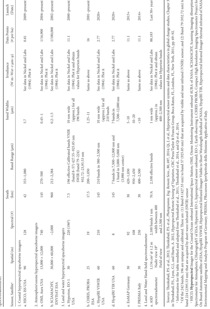
hyperspectral imagers for Ocean, Atmosphere, and Land (Table 9.1). These include (Table 9.1) NASA’s Hyperion, HyspIRI, OMI, HICO, German’s EnMap, Italy’s PRISMA, ESA’s SCIAMACHY, and CHRIS PROBA (Miura and Yoshioka, 2012; Ortenberg, 2012; Qi et al., 2012). There are also current initiatives from pri vate industry in the commercial sector, like that from Boeing to launch hyperspectral sensors. The spatial, spectral, radiometric, and temporal characteristics of some of the key ocean, atmo spheric, and land observation spaceborne hyperspectral data are provided in Table 9.1.
9.2.8 Data Normalization Hyperspectral Data
We illustrate the hyperspectral data normalization taking the case of Hyperion data. The DNs of the Hyperion level 1 products are 16bit radiances and are stored as 16bit signed integers. The DNswere converted to radiances (W m−2 sr−1 µm−1) using an appropri
ate scaling (e.g., for a Hyperion image dated March 21, 2002, fac tor: 40 for visible and VNIR, and 80 for SWIR). However, users should check the header file of the image they work with to deter mine the exact scaling factor for their image.
Radiance (W m−2 sr−1 µm−1) for VNIR bands = DN/40 Radiance (W m−2 sr−1 µm−1) for SWIR bands = DN/80
Radiance to at-sensor top of atmosphere reflectance is then cal-culated using Reflectance (%) = n π θ λ λ L d ESUN cos S 2
where, TOA reflectance (atsatellite exoatmospheric reflectance)
Lλ is the radiance (W m−2 sr−1 µm−1)
d is the earthtosun distance in astronomic units at the acquisition date (see Markham and Barker, 1987)
ESUNλ is the irradiance (W m−2 sr−1 µm−1) or solar flux
(Neckel and Labs, 1984) θs is the solar Zenith angle
Note: θs is solar Zenith angle in degrees (i.e., 90° minus the sun
elevation or sun angle when the scene was recorded as given in the image header file).
Atmospheric correction methods include (1) dark object sub traction technique (Chavez, 1988), (2) improved dark object subtraction technique (Chavez, 1989), (3) radiometric normal ization technique: Bright and dark object regression (Elvidge et al., 1995), and (4) 6S model (Vermote et al. 2002). Readers with further interest in this topic are referred to Chapters 4 through 8 in Remotely Sensed Data Characterization, Classification, and Accuracies and Chander et al. (2009).
9.3 Data Mining and Data Redundancy
of Hyperspectral Data
Data mining is one of the critical first steps in hyperspectral data analysis. The primary goal of data mining is to eliminate redundant data and retain only the useful data. Data volumes
are reduced through data mining methods such as feature selection (e.g., principal component analysis (PCA), deriva tive analysis, and wavelets), lambdabylambda correlation plots (Thenkabail et al., 2000), minimum noise fraction (MNF) (Green et al., 1988; Boardman and Kruse, 1994), and HVIs (e.g., Thenkabail et al., 2014). Data mining methods lead to (Thenkabail et al., 2012b) (1) reduction in data dimensionality, (2) reduction in data redundancy, and (3) extraction of unique information.
It is a wellknown fact that wavebands adjacent to one another (e.g., 680 nm versus 690 nm or 550 nm versus 560 nm) are often highly correlated for a given application. In various research papers, Thenkabail et al. (2000, 2004a,b, 2010, 2012b, 2014), Numata (2012), and Thenkabail and Wu (2012) showed that in a large stack of 242 bands in a Hyperion data, typically ~10% of the wavebands (~20 bands) are very useful in agri cultural cropland or vegetation studies. It means for any one given application (e.g., agriculture), a large number of bands are likely to be redundant. So, the goal of the data mining is to identify and eliminate redundant bands. This will help elimi nate unnecessary processing of redundant data, at the same time retaining the optimal power of hyperspectral data. This process is of great importance at a time when “big data” are the norm of the times.
However, eliminating redundant bands needs to be done with considerable care and expertise. What is redundant for one application (e.g., agriculture; [Yao et al., 2011]) may be critical for another application (e.g., geology).
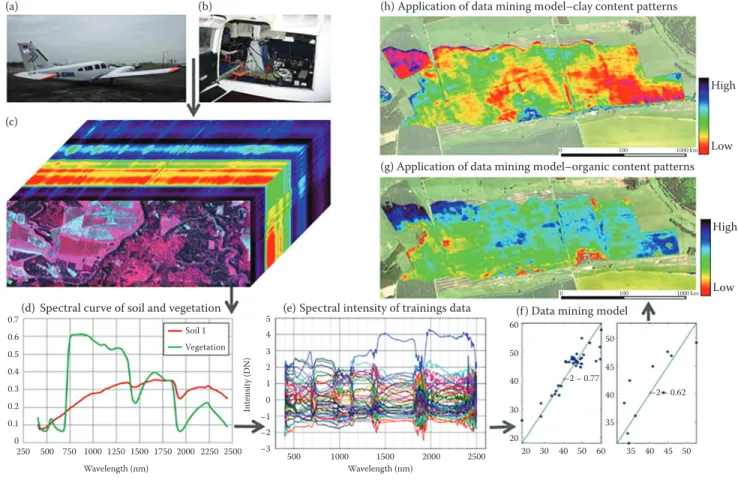
Data mining requires merging of different disciplines such as digital imagery, pattern recognition, database, artificial intelligence, machine learning, algorithms, and statistics. There are various models of data mining. The generic concept of data mining is illustrated in Figure 9.8 (Lausch et al., 2014). Figure 9.9 (Lausch et al., 2014) shows data mining model applications for studies in soil clay content and soil organic content.
9.4 Hughes’ Phenomenon and
the Need for Data Mining
If the number of bands remains high, the number of observa tions required to train a classifier increases exponentially to maintain classification accuracies, which is called Hughes’s phenomenon (Thenkabail and Wu, 2012). For example, Thenkabail et al. (2004a, b) used 20 Hyperion bands to clas sify five crop types and achieve an accuracy of 90%. Relative to this, the sevenband Landsat data provided only an accuracy of 60% in classifying the same five crops. However, the num ber of observation points (e.g., ground data) to train and test the algorithms will be exponentially higher for the Hyperion data relative to Landsat data because larger numbers of bands are involved with Hyperion. So, one needs to weigh the higher classification accuracies achieved using greater number of bands versus the resources required to gather exponentially
Ta bl e 9 .1 C ha ra ct er ist ic s o f S pa ce bo rne H yp er sp ec tr al S en so rs (E ith er in O rb it or P la nne d fo r L au nc h) fo r O ce an , A tm os ph ere , L and , a nd W at er A pp lic at io ns C om pa re d w ith A SD Sp ec tr or ad io m et er a Sen so r, Sa te lli te c Sp at ia l (m) Sp ec tra l (#) Swa th (k m) Ba nd R an ge ( μ m) ba nd W id th s ( μ m) Ir radi an ce (W m−Wsr−r μ m− μ ) D at a P oin ts (# p er h a) La un ch (D at e) 1. C oa sta l h yp er sp ec tra l s pace bo rn e im ag er s a. HI CO , ISS USA 90 128 42 353–1,080 5.7 Se e d at a in N ec ke l a nd L abs (1984). P lo t i t 0.81 2009–p res en t 2. A tm os ph er e\o zo ne h yp er sp ec tra l s pace bo rn e im ag er s a. O MI, A ura USA 13,000 × 12,000 740 145 270–500 0.45–1 Se e d at a in N ec ke l a nd L abs (1984). P lo t i t 1/16,900 2004–p res en t b. SCI AMA CHY , ENVISA T ESA 30,000 × 60,000 ~ 2,000 960 212–2,384 0.2–1.5 Se e d at a in N ec ke l a nd L abs (1984). P lo t i t 1/180,000 2002–p res en t 3. L an d an d wa ter h yp er sp ec tra l s pace bo rn e im ag er s a. H yp er io n, EO 1 USA 30 220 (196 b) 7.5 196 eff ec tiv e C ali bra te d ba nd s VNIR (b an d 8–57) 427.55–925.85 nm SWIR (b an d 79–224) 932.72–23,95.53 nm 10 nm w ide (a pp ro x.) fo r a ll 196 b an ds Se e d at a in N ec ke l a nd L abs (1984). P lo t i t a nd o bt ain va lues fo r H yp er io n ba nd s 11.1 2000–p res en t b. CHRIS, P RO BA ESA 25 19 17.5 200–1,050 1.25–11 Sa m e a s a bo ve 16 2001–p res en t c. H ys pIRI V SWIR USA 60 210 145 210 b an ds in 380–2,500 nm 10 nm w ide (a pp ro x.) fo r a ll 210 b an ds Se e d at a in N ec ke l a nd L abs (1984). P lo t i t 2.77 2020+ d. H ys pIRI TIR USA 60 8 145 7 ba nd s in 7,500–12,000 nm an d 1 b an d in 3,000–5,000 nm (3,980 nm cen ter) 7 ba nd s i n 7, 50 0– 12 ,0 00 n m Se e d at a in N ec ke l a nd L abs (1984). P lo t i t 2.77 2020+ e. EnMAP G er m an y 30 92 30 420–1,030 5–10 Sa m e a s a bo ve 11.1 2015+ 108 950–2,450 10–20 f. PRIS MA It al y 30 250 30 400–2,500 <10 Sa m e a s a bo ve 11.1 2014+ 4. L an d an d W at er H an d he ld sp ec tro radio m et er a. A SD sp ec tro radio m et er 1,134 cm 2 @ 1.2 m N adir v ie w 18° Fie ld o f v ie w 2,100 b an ds 1 nm w id th b et w een 400 an d 2,500 nm N/A 2,100 eff ec tiv e b an ds 1 nm w ide (a pp ro x.) in 400–2,500 nm Se e d at a in N ec ke l a nd L abs (1984). P lo t i t a nd o bt ain va lues fo r H yp er io n ba nd s 88,183 La st 30+ y ea rs So ur ce s: Th en ka ba il, P. S. et al ., 2 01 2; Th en ka ba il, P. S. et al ., Ph ot ogr am m . E ng . R em ot e Se ns ., 8 0, 6 97 , 2 01 4; Q i, J. et al ., H yp er sp ec tra l s en so r s ys te m s a nd d ata ch ar ac te ris tic s i n gl ob al ch an ge st ud ie s, Ch ap te r 3 , in Th en ka ba il, P. S. , L yo n, G .J. , a nd H ue te , A . 2 01 2, H yp er sp ec tra l R em ot e Se ns in g o f V eg eta tio n , C RC P re ss /T ay lo r & F ra nc is G ro up , B oc a R at on , F L, L on do n, F L, N ew Y or k, 2 01 1, p p. 6 9– 92 . a Inf or m at io n fo r t he ta ble m odifie d an d ado pt ed fr om Th en ka ba il et a l., 2011, Th en ka ba il et a l., 2014, an d Qi et a l., 2014. b Of th e 242 b an ds, 196 ar e uniq ue an d ca lib ra te d. Th es e a re: (1) B an d 8 (427.55 nm) to b an d 57 (925.85 nm) th at ar e acq uir ed b y vi sib le an d ne ar inf ra re d (VNIR) sen so r; an d (2) B an d 79 (932.72 nm) to ba nd 224 (2395.53 nm) th at ar e acq uir ed b y sh or t wa ve inf ra re d (SWIR) sen so r c HI CO , H yp ers pe ct ra l I m ag er fo r t he C oa sta l O ce an o nb oa rd In ter na tio na l S pace S ta tio n; O MI, O zo ne M oni to rin g In str um en t o nb oa rd A UR A o f N A SA; SCI AMA CHY , S ca nnin g Im ag in g Abs or pt io n Sp ec tro m et er fo r A tm os ph er ic CH ar tog ra phY o f ESA; H yp er io n EO 1, h yp er sp ec tra l s en so r o nb oa rd; EO 1, E ar th o bs er vin g 1; CHRIS P RO BA, C om pac t H ig h Res ol ut io n Im ag in g Sp ec tro m et er P ro je ct fo r On B oa rd A ut on om y s at el lit e o f ESA; H ys pIRI V SWIR , H yp er sp ec tra l I nf ra re d Im ag er V isi ble to Sh or t W av elen gt h Inf raR ed o f N A SA; H ys pIRI TIR , H yp er sp ec tra l I nf ra re d Im ag er th er m al inf ra re d of N A SA; En vir onm en ta l M ap pin g an d A na lysi s P rog ra m o f G er m an y; P RIS MA, P Re cur so re Ip erS pet tra le de lla M issio ne A pp lic at iva o f I ta ly.
higher number of observation (e.g., ground data) required to train and test the algorithms. So, higher accuracy by as much as 30% using 20 hyperspectral narrowbands (HNBs) when compared with sevenband Landsat will justify the greater number of ground data required. However, beyond 20 bands, increase in accuracy per increase in wavebands becomes asymptotic (e.g., Thenkabail et al., 2004a,b, 2012b). These studies, for example, show that when 40 Hyperion bands were used, the classification accuracies increased only by another 5% (from 90% with 20 bands to 95% with 40 bands). Here using 20 additional Hyperion bands (from 20 to 40) cannot be justified since the ground observation needed to train and test the algorithm will also increase exponential for 40 bands relative to 20. So, the key aim is to balance the higher clas sification accuracies with an optimal number of bands such as 20 instead too few or too many (e.g., 7 or 40). By doing so, we achieve a number of goals:
1. Increased classification accuracies with optimal number of bands.
2. Significantly reduced data redundancies with optimal number of bands.
3. Overcoming Hughes’s phenomenon by using optimal number of bands (e.g., 20) in which observation data (ground data) to train and test the algorithms will be kept to reasonable levels.
9.5 Methods of Hyperspectral
Data Analysis
Hyperspectral data analysis methods are broadly grouped under two categories (Bajwa and Kulkarni, 2012):
1. Feature extraction methods 2. Information extraction methods
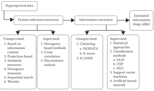
Under each of the earlier two categories, specific unsupervised and supervised classification approaches exist (Figure 9.10) (Bajwa and Kulkarni, 2012; Plaza et al., 2012). Methods of classi fying vegetation classes or crop types or vegetation species using HNBs are discussed extensively in this chapter and include unsu pervised classification, supervised approaches, spectral angle mapper (SAM), artificial neural networks, and support vector machines (SVMs), multivariate or partial least square regressions (PLSR), and discriminant analysis (Thenkabail et al., 2012a). Fundamental philosophies of hyperspectral data analysis involve two approaches:
1. Optimal hyperspectral narrowbands (OHNBs) where only a selective number of nonredundant bands are used (e.g., ~20 off Hyperion OHNBs are used).
2. Whole spectral analysis (WSA) where all the bands in the continuum (e.g., all 242 Hyperion bands in 400–2500 nm) are used. Data mining-system (DM-S) Iterative process Knowledge Validation phase Test phase Training phase Trainings
data Referencevalue Testdata Reverencevalue Validationdata Referencevalue Data preprocessing Data postprocessing Determined quality Evaluation Estimated value + (–1) Estimated value Error Feature selection and extraction Classifier application Data preprocessing Data preprocessing Feature selection and extraction Classifier optimization Data preprocessing Data preprocessing Feature selection and extraction Modelling Optimization Classifier training Data
Figure 9.8 Data mining 1. Data mining and linked open data—New perspectives for data analysis in environmental research. Data mining process with the data mining system (DMS) in the phases: (1) training phase, (2) test phase, and (3) validation phase. The data mining process works in a comparable way in all types of data mining types like text mining or web mining (changed according to Fayyad et al., (1996) and Tanner (2013). (From Lausch, A. et al., Ecol. Model., 2014.)
9.6 Optimal Hyperspectral Narrowbands
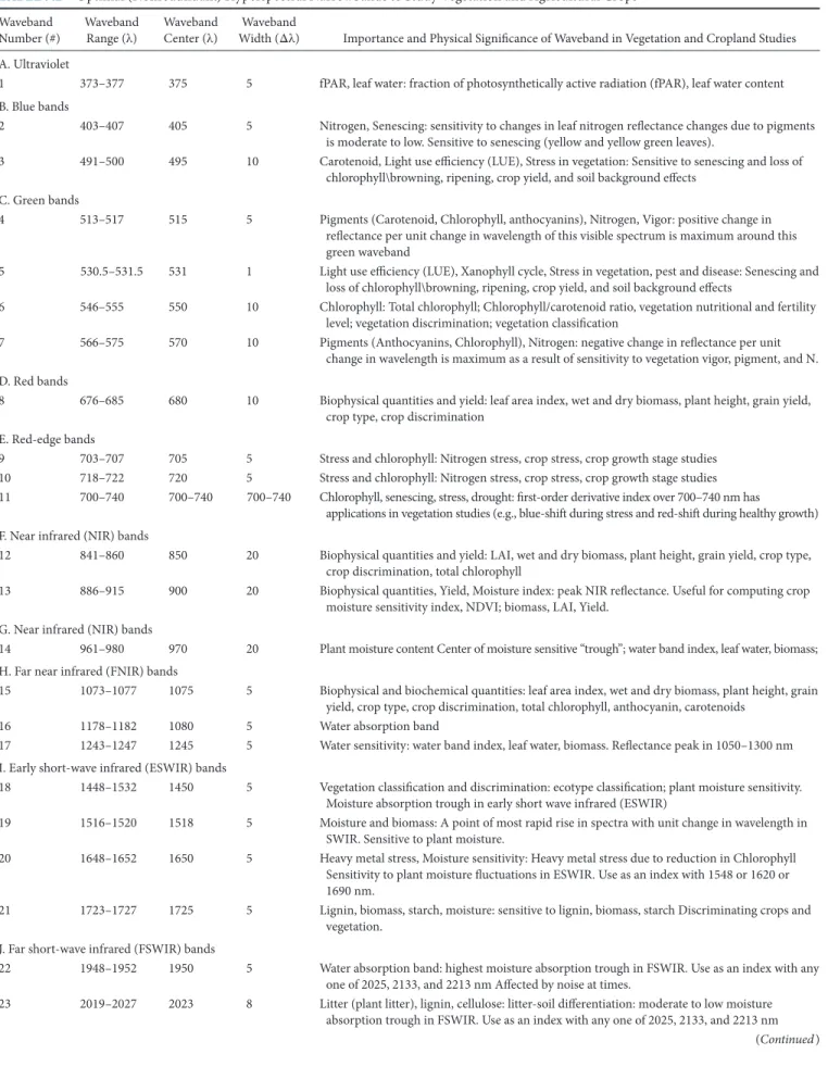
Determining wavebands that are optimal for different studies requires a thorough study of these subjects. For example, the impor tance of the wavebands for different studies such as vegetation, geol ogy, and water are all different. So, determining optimal OHNBs requires subject knowledge and considerable experience working with hyperspectral data. Based on the synthesis of the extensive studies conducted by Thenkabail et al. (2000, 2002, 2004a,b, 2012, 2013, 2014), the OHNBs for agriculture and vegetation studies are established and presented in Table 9.2. Each of these HNBs is iden tified for their importance in studying one or more of vegetation and crop biophysical and biochemical characteristics. Most of these bands are also very distinct from one another; so none of them are redundant. Using some combination of these bands will help better quantify the biophysical and biochemical characteristics of vegeta tion and agricultural crops (Alchanatis and Cohen, 2012; Pu, 2012). In the following sections and subsections, we will demonstrate how these HNBs are used in classifying, modeling, and mapping agri cultural croplands and other vegetation.Table 9.2 shows that over 400–2500 nm range of the spec
trum, there are 28 bands (e.g., ~12% of the 242 Hyperion bands
in 400–2500 nm range) that are optimal in the study of agri culture and vegetation. However, the redundant bands here (i.e., agriculture and vegetation applications) may be very useful in other applications such as geology (BenDor, 2012). For example, the critical absorption bands for studying min erals like biotite, kaolinite, hematite, and others are shown in Table 9.3. Unlike the vegetation and cropland bands, the HNBs required for mineralogy are quite different (Vaughan et al., 2011; Slonecker, 2012).
The earlier fact clearly establishes the need to determine OHNBs that are application specific.
9.7 Hyperspectral Vegetation Indices
One of the most common, powerful, and useful form of feature selection methods for hyperspectral data is based on the calcula tion of HVIs (Clark, 2012; Colombo et al., 2012; Galvão, 2012;60 50 40 30 35 40 –2 – 0.77 –2 – 0.62 45 50 20 20 30 40 50 60 35 40 45 50 High Low Application of data mining model–organic content patterns (g)
(h) Application of data mining model–clay content patterns (b)
(a)
(c)
Data mining model (f)
High
Low
0 100 1000 km
0 100 1000 km
(d) Spectral curve of soil and vegetation 0.7 Soil 1 Vegetation 0.6 Refle ct an ce 0.5 0.4 0.3 0.2 0.1 0 250 500 750 1000 1250 Wavelength (nm) 500 1000Wavelength (nm)1500 –3 –2 –1 0 1 2 3 In te ns ity (D N ) 4
(e) Spectral intensity of trainings data 5
2000 2500
1500 1750 2000 2250 2500
Figure 9.9 Data mining 2. (a, b) Data mining and linked open data—New perspectives for data analysis in environmental research. Airborne hyperspectral AISAEagle/HAWK remote sensor mounted on Piper, (c) CIRimage from hyperspectral sensors of the AISAEAGLE/ HAWK (AISADUAL) 400–2500 nm with data cube, 367 spectral bands with 2 m recorded ground resolution, date of recording Mai 2012 with a Piper, Region Schäfertal—Bode Catchment, (d) Spectral curve of ground truth sampling points for soil and vegetation in the test site. (e) Spectral intensity curves of imaging hyperspectral data, (f) data mining model, (g) application of the best data mining model on airborne hyperspectral image data for quantification and recognition of organic content patterns, and (h) pattern of clay content. (From Lausch, A. et al., Ecol. Model., 2014.)
Gitelson, 2012a,b; Roberts, 2012). The HVIs achieve two impor tant goals of hyperspectral data analysis:
1. Compute many specific targeted HVIs to help model bio physical and biochemical quantities.
2. Reduce the data volume (mine the data) to eliminate all redundant bands for a given application.
There are several approaches to deriving HVIs. These are briefly presented and discussed.
9.7.1 Two-Band Hyperspectral
Vegetation Indices
The twoband hyperspectral vegetation indices (TBHVIs) are defined as follows (Thenkabail et al., 2000):
TBHVI R R R R ij j i j i =
(
−)
+(
)
(9.1)where, i, j = 1 … N, with N = number of narrowbands. Hyperion 242 bands offer the possibility of 29,161 unique indices (242 * 242 =
58,564 − 242 = 58,322 divided by 2 resulting in C2422 = 29,161;
−242 because the values on the diagonal of matrix of 242 * 242 are unity, divided by 2 because the values above the diagonal of the matrix and below the diagonal of matrix are transpose of one another). However, as defined in Section 9.2.3, only 157 of the 242 Hyperion bands are useful after removing the wavebands in the atmospheric windows and those that are uncalibrated. This will
still leave C1572 = 12,246 unique TBHVIs.
Any one of the crop biophysical or biochemical quantity (e.g., biomass, leaf area index, nitrogen) is correlated with each one of the 12,246 TBHVIs (Stroppiana et al., 2012; Zhu et al., 2012). This will result for each crop variable (e.g., biomass) a
total of 12,246 unique models, each providing an Rsquare. Figure 9.11 shows the contour plot of 12,246 Rsquare values plotted for (1) rice crop wet biomass with TBHVIs (Figure 9.11; above the diagonal) and (2) barley crop wet biomass with TBHVIs (Figure 9.11, below the diagonal). The areas with “bull’seye” are regions of rich information having high Rsquare values, whereas the areas in gray are redundant bands
with low Rsquare values. Based on these lambda (λ1) versus
lambda (λ2) plots (Figure 9.11), the optimal waveband centers
(λ) and widths (Δλ) are determined (Table 9.2). Table 9.2 shows the optimal wavebands (λ), wavebands centers (λ), and widths (Δλ) based on numerous studies (Thenkabail et al., 2000, 2002, 2004a,b, 2012, 2013, 2014), and a metaanalysis of these studies. 9.7.1.1 Refinement of Two-Band HVIs
Further refinement of each of the twoband HVIs (TBHVIs) is possible by computing (1) soiladjusted versions of TBHVIs and (2) atmospheric corrected versions of TBHVIs. Interested read ers can read more on this topic at Thenkabail et al. (2000).
9.7.2 Multi-Band Hyperspectral
Vegetation Indices
The multiband hyperspectral vegetation indices (MBHVIs) are computed as follows (Thenkabail et al., 2000; Li et al., 2012):
MBHVIi a Rij j j 1 N = =
∑
(9.2) whereMBHVIi is the crop variable i
R is the reflectance in bands j (j = 1 − N with N = 242 for Hyperion)
a is the coefficient for reflectance in band j for ith variable Hyperspectral data Feature selection/extraction Unsupervised: 1. Divergence based methods 2. Cross correlation 3. Discriminant analysis Supervised: 1. Statistical approaches 2. Classification methods a. SAM b. OSP c. MLC 3. Support vector machines 4. Artificial neural network 1. Clustering a. ISODATA b. K-mean 2. ICAMM
Information extraction informationEstimated (map, table) Unsupervised: Supervised: 1. Based on information content 2. Projection-based 3. Similarity measures 4. Divergence measures 5. Sequential search 6. Wavelet
Figure 9.10 Hyperspectral data analysis methods. (From Bajwa, S. and Kulkarni, S.S., Hyperspectral data mining, Chapter 4, in Thenkabail, P.S., Lyon, G.J., and Huete, A., Hyperspectral Remote Sensing of Vegetation, CRC Press/Taylor & Francis Group, Boca Raton, FL/London, U.K./New York, 2012, pp. 93–120.)
Table 9.2 Optimal (Nonredundant) Hyperspectral Narrowbands to Study Vegetation and Agricultural Cropsa, b, c Waveband
Number (#) Waveband Range (λ) Waveband Center (λ) Width (Δλ) Waveband Importance and Physical Significance of Waveband in Vegetation and Cropland Studies A. Ultraviolet
1 373–377 375 5 fPAR, leaf water: fraction of photosynthetically active radiation (fPAR), leaf water content
B. Blue bands
2 403–407 405 5 Nitrogen, Senescing: sensitivity to changes in leaf nitrogen reflectance changes due to pigments
is moderate to low. Sensitive to senescing (yellow and yellow green leaves).
3 491–500 495 10 Carotenoid, Light use efficiency (LUE), Stress in vegetation: Sensitive to senescing and loss of
chlorophyll\browning, ripening, crop yield, and soil background effects C. Green bands
4 513–517 515 5 Pigments (Carotenoid, Chlorophyll, anthocyanins), Nitrogen, Vigor: positive change in
reflectance per unit change in wavelength of this visible spectrum is maximum around this green waveband
5 530.5–531.5 531 1 Light use efficiency (LUE), Xanophyll cycle, Stress in vegetation, pest and disease: Senescing and
loss of chlorophyll\browning, ripening, crop yield, and soil background effects
6 546–555 550 10 Chlorophyll: Total chlorophyll; Chlorophyll/carotenoid ratio, vegetation nutritional and fertility
level; vegetation discrimination; vegetation classification
7 566–575 570 10 Pigments (Anthocyanins, Chlorophyll), Nitrogen: negative change in reflectance per unit
change in wavelength is maximum as a result of sensitivity to vegetation vigor, pigment, and N. D. Red bands
8 676–685 680 10 Biophysical quantities and yield: leaf area index, wet and dry biomass, plant height, grain yield,
crop type, crop discrimination E. Rededge bands
9 703–707 705 5 Stress and chlorophyll: Nitrogen stress, crop stress, crop growth stage studies
10 718–722 720 5 Stress and chlorophyll: Nitrogen stress, crop stress, crop growth stage studies
11 700–740 700–740 700–740 Chlorophyll, senescing, stress, drought: firstorder derivative index over 700–740 nm has
applications in vegetation studies (e.g., blueshift during stress and redshift during healthy growth) F. Near infrared (NIR) bands
12 841–860 850 20 Biophysical quantities and yield: LAI, wet and dry biomass, plant height, grain yield, crop type,
crop discrimination, total chlorophyll
13 886–915 900 20 Biophysical quantities, Yield, Moisture index: peak NIR reflectance. Useful for computing crop
moisture sensitivity index, NDVI; biomass, LAI, Yield. G. Near infrared (NIR) bands
14 961–980 970 20 Plant moisture content Center of moisture sensitive “trough”; water band index, leaf water, biomass;
H. Far near infrared (FNIR) bands
15 1073–1077 1075 5 Biophysical and biochemical quantities: leaf area index, wet and dry biomass, plant height, grain
yield, crop type, crop discrimination, total chlorophyll, anthocyanin, carotenoids
16 1178–1182 1080 5 Water absorption band
17 1243–1247 1245 5 Water sensitivity: water band index, leaf water, biomass. Reflectance peak in 1050–1300 nm
I. Early shortwave infrared (ESWIR) bands
18 1448–1532 1450 5 Vegetation classification and discrimination: ecotype classification; plant moisture sensitivity.
Moisture absorption trough in early short wave infrared (ESWIR)
19 1516–1520 1518 5 Moisture and biomass: A point of most rapid rise in spectra with unit change in wavelength in
SWIR. Sensitive to plant moisture.
20 1648–1652 1650 5 Heavy metal stress, Moisture sensitivity: Heavy metal stress due to reduction in Chlorophyll
Sensitivity to plant moisture fluctuations in ESWIR. Use as an index with 1548 or 1620 or 1690 nm.
21 1723–1727 1725 5 Lignin, biomass, starch, moisture: sensitive to lignin, biomass, starch Discriminating crops and
vegetation. J. Far shortwave infrared (FSWIR) bands
22 1948–1952 1950 5 Water absorption band: highest moisture absorption trough in FSWIR. Use as an index with any
one of 2025, 2133, and 2213 nm Affected by noise at times.
23 2019–2027 2023 8 Litter (plant litter), lignin, cellulose: littersoil differentiation: moderate to low moisture absorption trough in FSWIR. Use as an index with any one of 2025, 2133, and 2213 nm
The process of modeling involves running stepwise linear regression models (e.g., using MAXR algorithm in Statistical Analysis System (SAS, 2009) with any one biophysical or bio chemical variable (e.g., biomass) as dependent variable and the numerous HNBs as independent variables (e.g., 157 of the 242 useful bands of Hyperion). In this modeling approach, we will get the best oneband, twoband, threeband, and so on to best nband model. The best oneband model is the one in which the biomass (taken as example) has highest Rsquare value with a single band out of the total 157 Hyperion HNBs. Then, we obtain the best twoband model, in which two HNBs provide a best Rsquare value with biomass. Similarly, the best threeband, best fourband, and best nband (e.g., all 157 Hyperion bands) models are obtained, even though, theoretically, all 157 bands can be involved in providing a 157band biomass model that is usually meaningless due to overfitting of data. However, a plot of Rsquare values (yaxis) versus the number of bands (xaxis) will show us when an increase in Rsquare values with the addi tion of wavebands becomes asymptotic. Alternatively, we can also consider additional bands, when there is at least an increase of 0.03 or higher in Rsquare value when additional bands are added. So, the approach we can use is to look at oneband model
and see its Rsquare. Then, when twoband model increases Rsquare value by at least 0.03 (a threshold we can set), then con sider the twoband model; otherwise, retain the oneband model as final. At some stage, we will notice that addition of a band does not increase Rsquare value by more than 0.03. Typically, we have noticed that anywhere between 3 and 10 HNBs explain optimal variability in most agricultural crop and vegetation variables. Beyond these 3–10 bands, the increase in Rsquare per increase in band is insignificant or asymptotic. However, which 3–10 bands within 400–2500 nm will, often, vary is based on the type of crop variable.
Through MBHVIs, we can establish the following:
1. How many HNBs are required to achieve an optimal Rsquare for any biophysical or biochemical quantity? 2. Which HNBs are involved in providing optimal Rsquare? 3. Through this process, we can determine which are impor tant HNBs and which are redundant. However, the best approach to achieve this is by a study conducted for many crops, involving several crop variables, and based on data from multiple sites and years. Table 9.2 provides one such summary.
Table 9.2 (continued ) Optimal (Nonredundant) Hyperspectral Narrowbands to Study Vegetation and Agricultural Cropsa, b, c Waveband
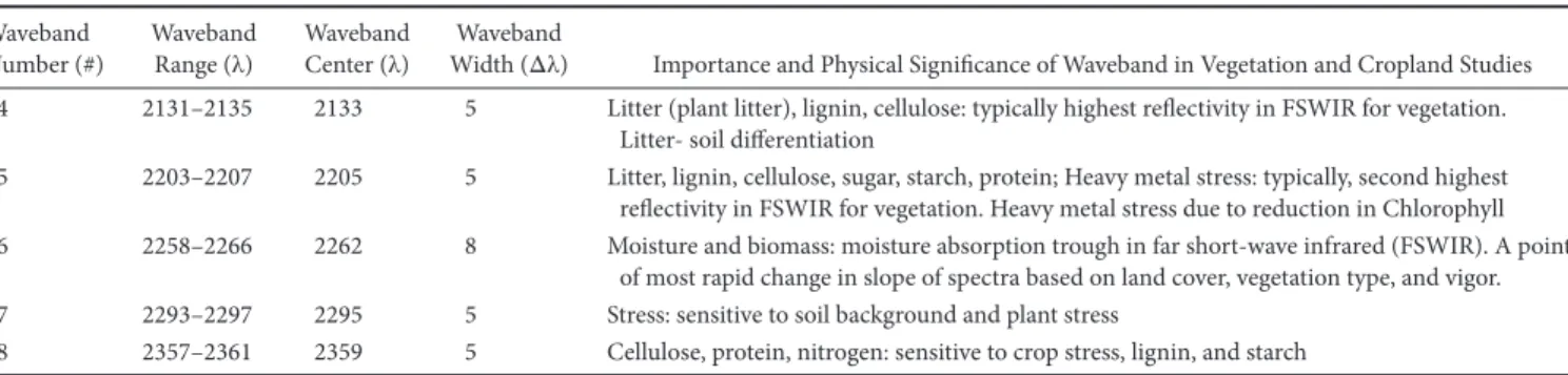
Number (#) Waveband Range (λ) Waveband Center (λ) Width (Δλ) Waveband Importance and Physical Significance of Waveband in Vegetation and Cropland Studies 24 2131–2135 2133 5 Litter (plant litter), lignin, cellulose: typically highest reflectivity in FSWIR for vegetation.
Litter soil differentiation
25 2203–2207 2205 5 Litter, lignin, cellulose, sugar, starch, protein; Heavy metal stress: typically, second highest reflectivity in FSWIR for vegetation. Heavy metal stress due to reduction in Chlorophyll
26 2258–2266 2262 8 Moisture and biomass: moisture absorption trough in far shortwave infrared (FSWIR). A point
of most rapid change in slope of spectra based on land cover, vegetation type, and vigor.
27 2293–2297 2295 5 Stress: sensitive to soil background and plant stress
28 2357–2361 2359 5 Cellulose, protein, nitrogen: sensitive to crop stress, lignin, and starch
Sources: Modified and adopted from Thenkabail, P.S. et al., Remote Sens. Environ., 71, 158, 2000; Thenkabail, P.S. et al. (2002); Thenkabail, P.S. et al., Remote Sens. Environ., 90, 23, 2004a; Thenkabail, P.S. et al., Remote Sens. Environ., 91, 354, 2004b; Thenkabail et al. (2012, 2013); Thenkabail, P.S. et al., Photogramm. Eng. Remote Sens., 80, 697, 2014.
a Most hyperspectral narrowbands (HNBs) that adjoin one another are highly correlated for a given application. Hence from a large number of HNBs, these nonredundant (optimal) bands are selected.
b These optimal HNBs are for studying vegetation and agricultural crops. When we use some or all of these wavebands, we can attain highest possible classi fication accuracies in classifying vegetation categories or crop types.
c Wavebands selected here are based on careful evaluation of large number of studies.
Table 9.3 Subpixel Mineral Mapping of a Porphyry Copper Belt Using EO1 Hyperion Data
Hyperion Band (#) Wavelength (nm) Feature Minerals Mineral Characteristic
210, 217 2254, 2324 Absorption Biotite Potassicbiotitic alteration zone
205 2203 Absorption Muscovite and illite Al–OH vibration in minerals with muscovite deeper absorption than illite
201, 205 2163, 2203 Absorption Kaolinite Al–OH vibration
14, 79, 205 487, 932, 2203 Absorption Goethite
14, 53, 205 487, 884, 2203 Absorption Hematite
79211205 932, 2264, 2203 Absorption Jarosite
201 2163 Absorption Pyrophyllite Al–OH and Mg–OH
218 2335 Absorption Chlorite Al–OH and Mg–OH
These MBHVIs take advantage of the key absorption and reflec tive portions of the spectrum (e.g., Figure 9.12; [Gnyp et al., 2014]). Taking advantage of four HNBs, two reflective (900 and 1050 nm) and two absorptive (955 and 1220 nm), Gnyp et al. constitute an MBHVI (Equation 9.1). In their paper, Gnyp et al. (2014) clearly demonstrate the significantly higher Rsquare values provided by such a multiband HVIs when compared with other twoband HVIs (e.g., in Figure 9.13, GnyLi has a much higher Rsquare value relative to other indices). Interesting and maybe noteworthy that while the typical saturation effect (lack of sensitivity) at higher biomass amounts is still present, it is evidently somewhat less severe with GnyLi than the others (except REP but it has lower r2). Also, research by Thenkabail et al. (2004a, b), Mariotto et al. (2013), and Marshall and Thenkabail (2014) has demonstrated that anywhere between 3 and 10 HNBs involved in multiband HVIs explain greatest variability in modeling various biophysical and biochemical quantities for various agricultural crops.
However, it needs to be noted that the specific band centers and band widths are not as definitive as shown in Figure 9.12 or/ and Equation 9.1. This is because, with crop type and crop grow ing conditions, the specific reflective maxima (900 and 1050 nm)
and reflective minima (955 and 1220 nm) shown in Figure 9.12 and Equation 9.1 can vary. For example, the moisture absorp tion maxima can be at 750, 760, 770, or 780 nm (Thenkabail et al., 2012, 2013) or can be at 755 nm as shown in Figure 9.12 and Equation 9.1. As a result, we performed metaanalysis of a number of papers to come with the recommendations of HNB centers and HNB widths (Table 9.2) that are optimal for use in HVI computations across crops and vegetation.
GnyLi R R R R R R R R = + 900 1050 955 1220 900 1050 955 1220 × × × × − (9.3)
9.8 The Best Hyperspectral Vegetation
Indices and Their Categories
Based on extensive research over the last decade (Thenkabail et al., 2000, 2002, 2004a,b, 2012, 2013, 2014), six distinct categories of twoband TBHVIs (Table 9.4) are considered most significant and important in order to study specific biophysical and biochemi cal quantities of agriculture and vegetation. Author recommends
0.95–1 2365 2305 2244 2184 2123 2063 2002 1942 1881 1821 1760 1699 1639 1578 1518 1457 1397 1336 1276 1215 1155 1094 1034 973 916 855 794 733 672 611 550 489 428 428 489 550 611 672 733 794 855 916 973 1034 1094 1155 1215 1276 1336 1397 Wavelength 1 (nm)
Rice crop: contour plot of R-square values between rice wet biomass vs. HVIs
Barley crop: contour plot of R-square values between barley wet biomass vs. HVIs
W aveleng th 2 (n m ) 1457 1518 1578 1639 1699 1760 1821 1881 1942 2002 2063 2123 2184 2244 2305 2365 0.9–0.95 0.85–0.9 0.8–0.85 0.75–0.8 0.7–0.75 0.65–0.7 0.6–0.65 0.55–0.6 < 0.50
Figure 9.11 Lambda (λ) versus Lambda (λ) plot of Rsquare values between wet biomass and hyperspectral vegetation indices (HVIs) for the rice crop (above the diagonal) and barley crop (below the diagonal).
1150 Wavelength (nm) 0.0 0.2 Refle ct an ce *100 (%) 0.4 Rlocal.min.1 Rlocal.min.2 Rabsolute.max Rlocal.max R1050 R900 Moisture related R955 R1220 Biomass related 0.6 950 750 550 350 1350 1550 1750
Figure 9.12 New index. Development and implementation of a multiscale biomass model using hyperspectral vegetation indices for winter wheat in the North China Plain. Reflectance of winter wheat and its characteristic peaks and troughs with the reflectance maxima and minima in the NIR and SWIR domains. These peaks were used to compute the VI GnyLi. R is the reflectance value (%) at a specific wavelength (nm). (From Gnyp, M.L. et al., Int. J. Appl. Earth Obs. Geoinf., 33, 232, 2014.)
y = 0.914*exp(8.979*x) R2 = 0.78 y = 0.033*exp(6.384*x) R2 = 0.49 y = 0.603*exp(8.831*x) R2 = 0.84 y = 464.907*exp(–3.687*x) R2 = 0.47 y = 1E-59*exp(0.188*x) R2 = 0.70 y = 0.011*exp(7.007*x) R2 = 0.44 L1 L2 L3 L4 15 (a) (b) (c) (d) O bs er ve d bioma ss (t/ha) O bs er ve d bioma ss (t/ha) (e) (f) 10 5 0 15 10 5 0 15 10 5 0 15 10 5 0 –0.2 0.0 0.2 NRI 0.4 15 10 5 0 0.0 0.0 0.2 0.4 0.6 NDVI TCl 2.0 1.5 1.0 0.2 0.4 0.6 OSAVI 0.8 2.5 0.8 1.0 0.2 GnyLi 0.4 15 10 5 0 720 725 730 REP 735
Figure 9.13 Observed biomass versus various HVIs and also GnyLi (see Figure 9.20). R is the reflectance value (%) at a specific wavelength (nm). (From Gnyp, M.L. et al., Int. J. Appl. Earth Obs. Geoinf., 33, 232, 2014.)
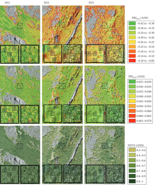
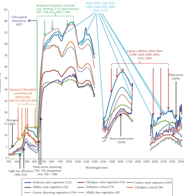
that in future, researchers use these HVIs, derived using HNBs, for their studies to quantify and model biophysical and biochemi cal quantities of various agricultural crops and vegetation of dif ferent types. The values of two such indices are illustrated. These are (1) hyperspectral biomass and structural index 1 (HBSI1; Thenkabail et al., 2014), derived using the Hyperion bands cen tered around 855 and 682 nm (each with 10 nm width), is applied to an agricultural area to determine biomass (Figure 9.14); and (2) photochemical reflectance index (PRI) for stress detection (e.g., Figure 9.15; Middleton et al., 2012). The importance of wavebands in computing the indices for various biophysical and biochemi cal is illustrated in Figure 9.16. Reader is encouraged to compare Figure 9.15 with Table 9.4 and Table 9.2 for better understand ing of HNBs (Table 9.2), HVIs (Table 9.4), and their importance (Figure 9.16) in studies pertaining to crops and vegetation.
9.9 Whole Spectral Analysis
A number of chapters discuss the usefulness and utility of using whole spectra (e.g., continuous and entire spectra over 400–2500 nm) for analysis using such methods as PLSR, wavelet analysis, continuum removal, SAM, and spectral matching tech niques (SMTs) (Thenkabail et al., 2012).
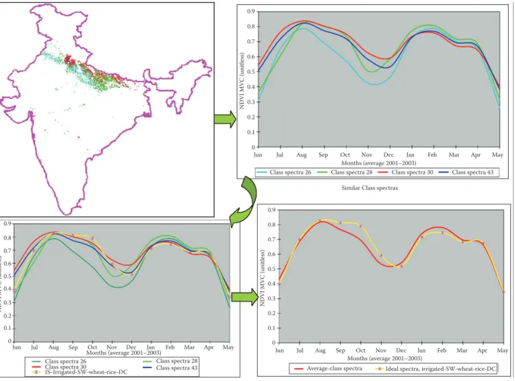
9.9.1 Spectral Matching Techniques
SMTs (Thenkabail et al., 2007) involves the following:1. Ideal or target spectral library creation: Collecting ideal or
target spectra (e.g., specific crops, specific species, specific mineral) and creating a spectral library.
2. Class spectra collection.
3. Matching class spectra with ideal spectra to identify and label classes.
The principal approach in SMT is to match the shape or the magnitude or (preferably) both to an ideal or target spectrum (pure class or “end member”). Thenkabail et al. (2007) proposed and implemented SMT for multitemporal data illustrated later (Figure 9.17). The qualitative phenoSMT approach concept remains the same for hyperspectral data (replace the number of bands of temporal data with the number of hyperspectral bands).
The quantitative SMTs consist of (Thenkabail et al., 2007) (1) spectral correlation similarity—a shape measure; (2) spectral similarity value—a shape and magnitude measure; (3) Euclidian distance similarity—a distance measure; and (4) modified spec tral angle similarity—a hyper angle measure.
9.9.2 Continuum Removal through Derivative
Hyperspectral Vegetation Indices
The derivative hyperspectral vegetation indices (DHVIs) are computed by integrating index over a certain wavelength (e.g., 600–700 nm or 700–760 nm). The equation is
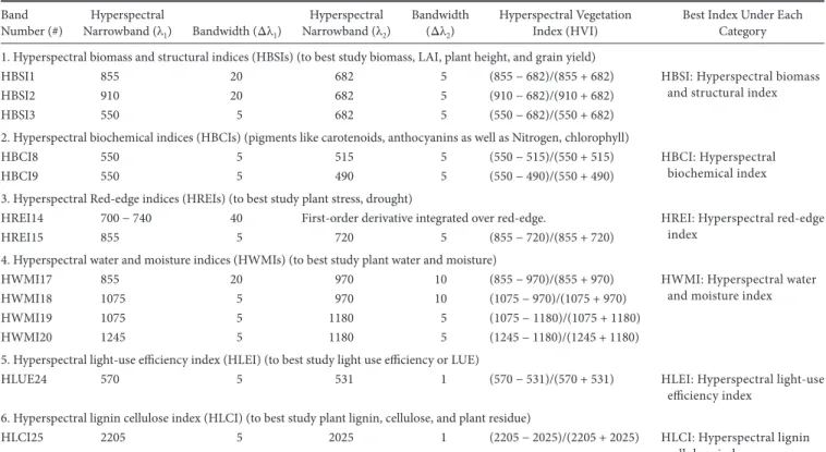
Table 9.4 Hyperspectral Vegetation Indices or HVIs Band
Number (#) Narrowband (λHyperspectral 1) Bandwidth (Δλ1)
Hyperspectral Narrowband (λ2)
Bandwidth (Δλ2)
Hyperspectral Vegetation
Index (HVI) Best Index Under Each Category 1. Hyperspectral biomass and structural indices (HBSIs) (to best study biomass, LAI, plant height, and grain yield)
HBSI1 855 20 682 5 (855 − 682)/(855 + 682) HBSI: Hyperspectral biomass
and structural index
HBSI2 910 20 682 5 (910 − 682)/(910 + 682)
HBSI3 550 5 682 5 (550 − 682)/(550 + 682)
2. Hyperspectral biochemical indices (HBCIs) (pigments like carotenoids, anthocyanins as well as Nitrogen, chlorophyll)
HBCI8 550 5 515 5 (550 − 515)/(550 + 515) HBCI: Hyperspectral
biochemical index
HBCI9 550 5 490 5 (550 − 490)/(550 + 490)
3. Hyperspectral Rededge indices (HREIs) (to best study plant stress, drought)
HREI14 700 − 740 40 Firstorder derivative integrated over rededge. HREI: Hyperspectral rededge
index
HREI15 855 5 720 5 (855 − 720)/(855 + 720)
4. Hyperspectral water and moisture indices (HWMIs) (to best study plant water and moisture)
HWMI17 855 20 970 10 (855 − 970)/(855 + 970) HWMI: Hyperspectral water
and moisture index
HWMI18 1075 5 970 10 (1075 − 970)/(1075 + 970)
HWMI19 1075 5 1180 5 (1075 − 1180)/(1075 + 1180)
HWMI20 1245 5 1180 5 (1245 − 1180)/(1245 + 1180)
5. Hyperspectral lightuse efficiency index (HLEI) (to best study light use efficiency or LUE)
HLUE24 570 5 531 1 (570 − 531)/(570 + 531) HLEI: Hyperspectral lightuse
efficiency index 6. Hyperspectral lignin cellulose index (HLCI) (to best study plant lignin, cellulose, and plant residue)
HLCI25 2205 5 2025 1 (2205 − 2025)/(2205 + 2025) HLCI: Hyperspectral lignin
cellulose index Sources: Modified and adopted from Thenkabail, P.S. et al., Photogramm. Eng. Remote Sens., 80, 697, 2014.
DHVI n i j I =
∑
λ ρ λ′( )
− ′ρ λ( )
λ λ ( ( 1∆ (9.4) wherei and j are band numbers λ is the center of wavelength
The process of obtaining DHVI value for 600–700 nm is as fol
lows: (1) DHVI1 = lambda 1 (e.g., λ1 = 600 nm) versus lambda
2 (e.g., λ2 = 610 nm). The difference in the reflectivity of these
two bands is then divided by their bandwidth (ΔλI = 10 nm)
and (2) DHVI2 = the process is repeated for lambda 1 (e.g., λ1
= 610 nm) versus lambda 2 (e.g., λ2 = 620 nm). The difference
in reflectivity of these two bands is then divided by their band
width (ΔλI = 10 nm) and (3) DHVIn = so on to lambda 1 (e.g.,
λ1 = 690 nm) versus lambda 2 (e.g., λ2 = 700 nm). The difference
in reflectivity of these two bands is then divided by their band
width (ΔλI = 10 nm). Finally, add DHVI1, DHVI2, and so on to
DHVIn to get single an integrated DHVI value over the entire 600–700 nm range.
The DHVIs can be derived over various wavelengths such as 400–2500 nm, 500–600 nm, 600–800 nm, and any other wavelength you find useful for the particular application. There are opportunities to further investigate the signifi cance of DHVIs over different wavelengths for a wide array of applications.
9.10 Principal Component Analysis
Another common, powerful, and useful feature selection method for hyperspectral data analysis is PCA. The PCA per forms following functions:1. Reduces data volumes: This happens since the PCA gen
erates numerous principal components (PCs) (as many as the number of wavebands), but the first few PCs explain almost all the variability of data. The first PC (PC1) explains the highest, followed by the other. Since each PC is constituted based on the information from all the bands (e.g., PC1 = factor loading for band 1 *
band 1 reflectivity + ⋯ + factor loading for band n *
band n reflectivity), the PCs have the power of hyper spectral bands, but does not have all the redundancy of the same.
2. Provides a new single band of information (e.g., PC1, PC2),
each of which (e.g., PC1) actually has the information derived from all the HNBs. These new bands of informa tion (e.g., PC1) can then be used to classify an area (e.g., to establish crop types) or used to model crop biophysical or biochemical quantities.
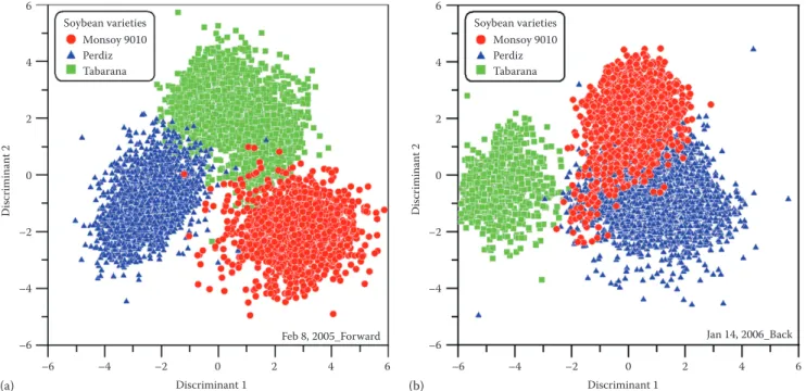
3. The power of PCs can be used to discriminate crop types,
or land cover themes, or species (e.g., Figure 9.18). Hyperion
(September 19, 2003) RGB Red: EO1_H_050
81°1΄30˝E 81°2΄15˝E 81°3΄0˝E 81°3΄45˝E
81°3΄45˝E
81°4΄30˝E
Hyperspectral biomass and structural index (HBSI) = (B50 – B33)/(B50 + B33)
HBSI1 1 5.62 2.56 1.17 0.53 0.24 0.11 0.05 0.02 0.01 0.004 0.002 N S E W 0.8 0.6 0.4 0.2 0 –0.2 –0.4 –0.6 –0.8 –1 Biomass (kg/m2) 16°50'15''N 0 0.5 1 2 km 16°51'0''N 16°51'45''N Green: EO1_H_033 Blue: EO1_H_020 81°4΄30˝E 16°50 ΄1 5˝N 16°51 ΄0 ˝N 16°51 ΄45˝ N 81°2΄15˝E 81°1΄30˝E 81°3΄0˝E
Figure 9.14 Spatial depiction of a hyperspectral biomass and structural index 1 (HBSI1) as applied to an agricultural area. One of the HVIs (HBSI1) in mapping wet biomass for a study area using Hyperion hyperspectral data. The red area in the zscale can be stretched further to show better biomass variability with change in HBSI1. For example, HBSI1 0.4 = 0.53 and HBSI 0.6 = 1.16, HBSI1 0.8 = 2.56, and HBSI1 = 5.62. The current stretch does not adequately show these differences (as much of the higher end is in red). However, if we stretch between HBSI1 from 0.4 to 1.0, then the biomass differences in this HBSI1 range, which is 0.53–5.62, will show up in better contrast. The relationship between HBSI1 and biomass is nonlinear due to saturation of indices at the higher end of the biomass. However, this saturation is much lower for hyperspectral index like HBSI1 when compared to broadband NDVI.
–0.42 to –0.38 SN3 SN2 SN1 –0.38 to –0.34 –0.34 to –0.30 –0.30 to –0.26 –0.26 to –0.22 –0.22 to –0.18 –0.18 to –0.14 –0.14 to –0.10 –0.10 to –0.06 0.025–0.030 0.030–0.035 0.035–0.040 0.040–0.045 0.045–0.050 0.050–0.055 0.055–0.060 0.060–0.065 0.065–0.070 0.3–0.4 NDVI (AHS) PRI570 (AHS) PRI512 (AHS) 0.4–0.5 0.5–0.6 0.6–0.7 0.7–0.8 0.8–0.9 0.9–1
Figure 9.15 Assessing structural effects on photochemical reflectance index (PRI) for stress detection in conifer forests. PRI512, PRI570, and NDVI obtained from the AHS airborne sensor from three study areas of Pinus nigra with different levels of stress: SN1, SN2, and SN3. At the bot tom of each image, two zoom images of a central plot, one pixel based displaying 1 × 1 and 3 × 3 resolutions and the other at object level. Note: PRI512 is a normalized index involving a waveband centered at 512 and 531 nm, whereas PRI570 is a normalized index involving a waveband centered at 570 and 531 nm. Airborne hyperspectral scanner (AHS) (Sensytech Inc., currently Argon St. Inc., Ann Arbor, MI) acquiring 2 m spatial resolution imagery in 38 bands in the 0.43–12.5 μm spectral range. (From HernándezClemente, R. et al., Adv. Space Res., 53, 440, 2011.)
9.11 Spectral Mixture Analysis
of Hyperspectral Data
Hyperspectral data have great ability to distinguish specific objects based on their unique signatures. For example, wheat versus barley crops are distinguished based on the spectral reflectivity in two HNBs, each of 10 nm wide, and centered at 687 and 855 nm (e.g., Figure 9.19). However, often, we find multiple objects or classes within a pixel. In situations like that, we will need to perform spec tral mixture analysis (SMA) and an independent component anal ysis, in order to unmix the spectral signatures within each pixel.
The reference spectra for SMA are derived from “end mem bers” (e.g., Figure 9.20). Once all the materials in the image are
identified, then it is possible to use linear or nonlinear spec tral unmixing to find out how much of each material is in each pixel.
The concept of unmixing hyperspectral data is illus trated by showing Hyperion unmixing of (1) vegetation frac tional cover in Figure 9.21 and (2) minerals in Figure 9.22. Subpixel mineral mapping of a porphyry copper belt using EO1 Hyperion data in Figure 9.23 involved mineral spec tra extracted from Hyperion compared to convolved spectra from field samples and reference library spectra (Figures 9.20 and 9.21; Hosseinjani Zadeh et al., 2014). Extensive discus sions on linear and nonlinear SMAs can be found in Plaza et al. (2012).
Plant stress (2295)
Heavy metal stress (1650)
Pigments (Chlorophyll, carotenoid, and
anthocyanin) (450, 515, 550, 570, 650)
Lignin, cellulose, plant litter (1548, 1620, 1690, 2025,
2133, 2205)
Water (970, 1180, 1245, 1450, 1760, 1950, 2050,
2145, 2173)
Biophysical quantity and yield (e.g., biomass, LAI, plant density) (687, 760, 855, 1045, 1100) Chlorophyll absorption (687) 65 60 55 50 45 40 35 Refle ct an ce (%) 30 25 20 15 10 5 0 350 450 550 650 950
Plant stress, senescing (705, 720, integration
over 700 = 740) Light use efficiency
(490, 531) 1050 1150 1250 1350 Wavelength (nm) 1450 1550 1650 1750 1850 1950 2050 2150 2250 2350 750 850 Nitrogen (405)
Soybeans, late vegetative (132) Chickpea, early vegetative (76) Cotton, early vegetative (105)
Alfalfa, early vegetative (35) Soybeans, critical (79) Chickpea, critical (56)
Cotton, flowering vegetative (134) Alfalfa, late vegetative (43)
Figure 9.16 Importance of various portions of hyperspectral data in characterizing biophysical and biochemical quantities of crops and vegetation.