Improving and validating methods in lesion behaviour mapping

(1)

Improving and validating methods in lesion behaviour mapping

Dissertation

zur Erlangung des Grades eines Doktors der Naturwissenschaften

der Mathematisch-Naturwissenschaftlichen Fakultät und

der Medizinischen Fakultät der Eberhard-Karls-Universität Tübingen

vorgelegt von

Christoph Sperber

Geboren in Kirchheim/Teck, Deutschland

(2)

Tag der mündlichen Prüfung: 18.12.2018

Dekan der Math.-Nat. Fakultät: Prof. Dr. W. Rosenstiel Dekan der Medizinischen Fakultät: Prof. Dr. I. B. Autenrieth

1. Berichterstatter: Prof. Dr. Dr. Hans-Otto Karnath

2. Berichterstatter: Prof. Dr. Martin Giese

Prüfungskommission: Prof. Dr. Dr. Hans-Otto Karnath

Prof. Dr. Martin Giese

Prof. Dr. Hanspeter Mallot

(3)

Declaration:

I hereby declare that I have produced the work entitled “Improving and validating methods in lesion behaviour mapping”, submitted for the award of a doctorate, on my own (without external help), have used only the sources and aids indicated and have marked passages included from other works, whether verbatim or in content, as such. I swear upon oath that these statements are true and that I have not concealed anything. I am aware that making a false declaration under oath is punishable by a term of imprisonment of up to three years or by a fine.

Tübingen, den ... ... Datum / Date Unterschrift /Signature

(4)

Abstract

The investigation of diseased brain is one of the major methods in cognitive neuroscience. This approach allows numerous insights both into human cognition and brain architecture. Most prominent is the method of lesion behaviour mapping, where inferences about functional brain architecture are drawn from focally lesioned brains. In the last 15 years, the state-of-the-art implementation of lesion behaviour mapping has been voxel-based lesion behaviour mapping, which is based on the framework of statistical parametric mapping. Recently, the validity of this method has been criticised and multivariate methods have been proposed to complement or even replace it.

In my thesis, I aim to evaluate these different methodological approaches to lesion behaviour mapping and to provide guidelines on how lesion-brain inference should be drawn. In my first empirical work, I investigate the validity of voxel-based lesion behaviour mapping. It shows that previous studies overestimated biases inherent to the method, and that validity can be improved by the use of correction factors. The second empirical work deals with a recently developed method of multivariate lesion behaviour mapping. On the one hand, I clarify how this method can be used to obtain valid lesion-brain inference. On the other hand, I show that the method is not able to overcome all limitations of voxel-based lesion behaviour mapping. In my last work, I apply multivariate lesion behaviour mapping to investigate the neural correlates of higher motor cognition. This analysis is the first to identify a brain network to underlie apraxia, a disorder of higher motor cognition, which underlines the benefits of the new multivariate approach in brain networks.

(5)

2

Acknowledgements

First, I would like to express my great appreciation to my advisor Prof. Hans-Otto Karnath for his supervision and guidance. All the great opportunities that he offered me were challenging, but in the end it turned out very well and it got me where I am now.

Besides my advisor, I would also like to thank the rest of my thesis committee for their guidance: Prof. Martin Giese and Prof. Hanspeter Mallot. I also would like to thank Prof. Georg Goldenberg for the cooperation on the topic of higher order motor control.

I would like to offer special thanks to the Friedrich Naumann Foundation for financial support, and even more for their ideal promotion.

I thank the members of the Section of Neuropsychology for all the team work and the great time we have had together. Special thanks go to Johannes Rennig, Bianca de Haan, Daniel Wiesen, Marc Himmelbach, Ina Baumeister, Sonja Cornelsen, Maren Prass, Gabriela Zaiser, Sophia Nestmann, and Jasmin Klopfer.

I am particularly grateful to Johannes Rennig and Bianca de Haan. Without their initial guidance, my scientific projects never would have gotten that far.

I also want to acknowledge the awesome and efficient cooperation with Daniel Wiesen.

It was a great honour to be accompanied by Hannah Tomczyk, who really isn’t that bad at all.

All moose were trained by Þōrvaldr Eirikssonr, and no moose were harmed or inappropriately nuzzled while performing my research.

(8)

5

1 Cognitive neuroscience and diseased brains

The scientific aim of cognitive neuroscience is to understand how the human brain works. A major part of this is to map the anatomo-behavioural architecture of the brain, that is to find out which brain regions are responsible for a certain cognitive behaviour. Until the middle of the 20th_{century, the mapping of deceased brain has}

been the only available method in this field. The neural correlates of a cognitive function were inferred from patients with focal neurologic damage, who suffered from deficits in the cognitive function.

In the last decades, new methods emerged. On the one hand, imaging techniques such as electro- or magnetoencephalography, positron emission tomography, and functional magnetic resonance imaging were established in the field. One important limitation of these imaging methods is that they might not only identify regions where activity is causal for a certain cognitive function, but also regions where activity is just correlative. On the other hand, non-invasive transcranial neurostimulation methods based on electric or magnetic stimulation of the brain came up. Latter methods allow drawing the conclusion if activity of certain brain regions is

necessary for a cognitive function. Unfortunately, transcranial neurostimulation is

limited to a few experimental protocols, to a few possible stimulation loci, and effects are often weak. Here, the mapping of diseased brains comes back into play. Brains with focal damage also offer the opportunity to study causality in brain-behaviour relations (Rorden & Karnath, 2004). This is the reason why the mapping of diseased brains is still an important method in cognitive neurosciences in the 21st_century.

The most common approach in mapping diseased brains involves the study of stroke patients, which was termed lesion behaviour mapping. My thesis deals with this method, and the greater goal of my work is to find the best way to perform lesion behaviour mapping. I investigate the validity of both established and novel methods in the field, I empirically define guidelines for novel methods, and I apply these methods to identify the networks underlying higher motor cognition.

In the synopsis of my thesis, I first give an introduction into the methods of lesion behaviour mapping in chapter 2. I outline the method’s historical evolution and depict procedures that are prerequisites for state of the art lesion behaviour mapping. Last, I provide an overview of the methodological paradigm that dominated lesion

(9)

6 behaviour mapping in the last 15 years: voxel-based lesion behaviour mapping. In chapter 3, I characterise several challenges and limitations in the field of voxel-based lesion behaviour mapping. Chapter 4 outlines an approach that is suited to investigate the impact of these limitations on the validity of lesion behaviour mapping, and which I used to investigate the different methods. Chapter 5 overviews a new method in the field: multivariate lesion behaviour mapping. This method is thought to overcome several of the limitations mentioned in the chapter before. In chapter 6, I provide a short overview on the empirical works in my thesis. Finally, in chapter 7, I picture possible future research directions in lesion behaviour mapping.

2 Lesion-deficit inference – from Paul Broca to statistical parametric

mapping

2.1 Early history

Historically, studies on patients with brain damage were the first studies ever to investigate the functional anatomy of the brain. One of the most famous milestones in the field dates back to the middle of the 19th_{century (Broca, 1861). In 1861, the}

French physician and anatomist Paul Broca heard about Louis Victor Leborgne, who suffered from a loss of speech production. This patient was unable to speak any words other than the syllable “tan”. Broca showed that both Leborgne’s cognitive capabilities and his ability to understand speech were largely preserved. When Leborgne died, Broca performed an autopsy and found the left inferior frontal cortex to be damaged. Broca replicated this finding in several other patients with deficient speech production, but intact comprehension. A general conclusion of these findings was relevant in providing a paradigm for future research: cognitive functions are anatomically localised in the brain.

For more than 100 years, the methodological approach used by Paul Broca - neurological single case studies with post mortem autopsy - was almost the only available method to investigate brain-function relationships. Some lesser known exceptions were the studies by Tatsuji Inouye (see Glickstein & Whitteridge, 1987) and by Gordon Holmes (Holmes & Lister, 1916). They studied patients with non-lethal gunshot wounds to the brain in the russo-japanese war and the First World War. By examining entry and exit wounds in the skull, they were able to map the primary visual cortex with high precision. The most innovative aspect about these studies was

(10)

7 the examination of a group of patients. Still, single case studies were the standard in the field, because anatomical information was usually only obtainable post mortem.

2.2 The advent of brain imaging and first lesion-behaviour mapping studies

In 1971, the first in vivo X-ray computed tomography scan of a human brain was carried out. Scanning and data processing, however, still took several hours, and the final image consisted of only one single low-resolution slice. Two years later, application of nuclear magnetic resonance in image generation was first described (Lauterbur, 1973) and used to obtain in vivo images in living organisms (Lauterbur, 1974). Based on these foundations, both X-ray computed tomography (CT) and magnetic resonance imaging (MRI) evolved at a tremendous pace into essential methods in many clinical fields, culminating in the Noble Prize awards of 1979 for Allan Cormack and Godfrey Hounsfield, and 2003 for Paul Lauterbur and Peter Mansfield.

The development of these imaging methods was of outstanding relevance for the diagnosis and treatment of stroke. CT allows to differentiate between ischaemic and haemorrhagic stroke, which is of vital significance in thrombolysis therapy (Freeman & Aguilar, 2012). Moreover, a wide array of more specialised CT or MRI clinical imaging protocols emerged, which allow to visualise brain perfusion, vessels, and diffusion (Jäger, 2000). Most importantly for the field of lesion behaviour mapping, structural CT or MRI that visualises the extent of stroke became available. For the first time in history, researchers were able to localize structural brain damage after stroke in vivo. This allowed researchers to perform anatomo-behavioural studies more efficiently than ever before on groups rather than single patients.

First anatomo-behavioural studies using these imaging methods qualitatively assessed brain damage. To do so, neuroradiologists – or other scientists with comparable expertise in brain anatomy and stroke imaging – visually inspected brain scans and assessed if certain areas were damaged. Alternatively, for a topographical approach, scientists manually transferred the lesion onto a template. In more detail, the lesion borders were drawn by hand on a schematic diagram of the brain, which could either be an over-simplified line drawing without any or only a few anatomical landmarks or any kind of brain template. Further analyses of these topographical data were performed qualitatively. For example, individual lesions were overlapped to identify brain areas that are often affected when a symptom is present.

(11)

8 This approach based on simple overlap topographies is however severely limited: brain regions often affected in patients with a symptom are not necessarily the neural correlates of the symptom, but instead areas that are simply more often affected in stroke in general (Rorden & Karnath, 2004). This issue can elegantly be visualised by computing a simple overlap of stroke patients in general, i.e. patients unselected for any symptom. In a study on 439 unselected acute right hemisphere stroke patients (Sperber & Karnath, 2016), we found overlap maxima in the centre of the territory of the middle cerebral artery, including Heschl’s gyrus, insula, and putamen. Overlap maxima are thus not specific in identifying a symptom’s neural correlates, but can originate from general stroke anatomy. The solution to this problem is the inclusion of control patients into the analysis (Rorden & Karnath, 2004). Control patients are stroke patients that do not suffer from the investigated symptom. The underlying rationale is that stroke in all patients follows its typical anatomy, however, only in the group of patients with the symptom the neural correlates of the symptom are damaged. Anatomo-behavioural studies should thus compare both groups. So-called lesion subtraction analysis (Rorden & Karnath, 2004) has often been used in this context. This analysis method requires normalised lesion data (see below, chapter 2.3.2). The analysis is computed for each voxel (= volumetric pixel), i.e. for each 3D imaging point, individually. For each voxel, in both groups the proportion of patients with damage in this voxel is identified. The difference between both proportional values now can indicate if a voxel is part of a symptom’s neural substrate. E.g., if a voxel is damaged in 60% of patients with the symptom, but in 15% of patients without the symptom (resulting in a difference of +45%), the voxel is assumed to be part of it. On the other hand, if a voxel is damaged in 60% of patients with the symptom, and also in 60% of patients without the symptom (resulting in a difference of 0%), the voxel is likely not neural substrate of the symptom. Latter example again illustrates how simple overlap analyses can be misleading, and why control patients are required in studies on patients with brain lesions.

2.3 Voxel-wise Statistical Mapping

Lesion subtraction analysis was an innovative method that lead to many new insights on brain architecture. Yet, it is only a qualitative approach. A more or less wide range of non-zero values is always present in a lesion subtraction analysis. Whether these values are just random stochastic fluctuations or indicative for an actual

(12)

brain-9 behaviour relation, is not obvious. This problem was overcome by the implementation of voxel-wise statistical mapping into the field of lesion behaviour mapping. Before I discuss the principles of this method, I need to introduce some pre-requisites that are commonly used for this method. Raw brain imaging obtained by CT or MR is not directly usable in voxel-wise lesion behaviour mapping. First, lesioned areas in the brain have to be identified, and second, the images have to be warped into a common space.

2.3.1 Lesion visualisation and delineation

Identification of damaged brain tissue after stroke is not a trivial task (for reviews see Provenzale et al., 2003; Merino & Warach, 2010). A first major issue is that we need to find an imaging modality that can be used to identify structurally damaged tissue. Optimal solutions, however, vary as a function of time since stroke, ranging from hyper-acute (~ first 48 hours after stroke) and acute (first 2 weeks after stroke), to chronic stroke (>3 months after stroke). When a patient with acute neurological symptoms arrives on a stroke unit, acquisition of brain imaging is a first important step in stroke diagnosis. Non-contrast CT is very sensitive to haemorrhagic stroke even in the early acute stage of stroke. On the other hand, ischemic stroke – with about 80% of stroke patients the most common stroke aetiology – often cannot be identified with acute CT in hyper-acute stroke. Furthermore, CT can fail to identify smaller stroke. Similarly, MR imaging has some limitations in acute stroke. T1-weighted MR imaging can achieve high imaging resolution, but it does not visualise acute structural damage at all. On the other hand, it is sensitive to chronic stroke. T2-weighted imaging can visualise acute stroke with a resolution that is superior to CT. In the hyper-acute stage, diffusion-weighted MR imaging can visualise the core ischemic zone, where diffusion broke down due to structural damage. Diffusion-weighted imaging, however, only provides low resolution, and can - to a minimal degree - be misleading about the extent of structural damage (Inoue et al., 2014a).

The challenge of stroke visualisation is not solved just by choosing the right imaging modality at the right time. More fundamental concerns arise in the comparison of acute versus chronic damage. In acute stroke, deficits might not only arise from structural damage, but also from diaschisis (Carrera & Tononi, 2014; Silasi & Murphy, 2014) and temporary malperfusion (Karnath et al., 2005; Zopf et al., 2012; Sebastian et al., 2014). In the chronic stage, brain architecture might be altered due to neural plasticity, i.e., the brain’s ability to reorganize its anatomo-behavioural

(13)

10 architecture in reaction to brain damage (e.g., Chelette et al., 2013; Vaina et al., 2014; Veldema et al., 2017). This hampers the transfer of findings in a clinical study to general anatomy of the healthy brain. Furthermore, post-stroke atrophy of brain tissue can limit the usability of chronic imaging to visualise structurally damaged areas and spatial normalisation (see below, chapter 2.3.2.). The complicated topic of choosing a time point of stroke imaging and behavioural assessment for lesion behaviour mapping was already discussed by several studies, including an own review paper (Karnath & Rennig, 2017; Shahid et al., 2017; de Haan & Karnath, 2018; Sperber & Karnath, 2018). We can summarise here that lesion visualisation for lesion behaviour mapping is not a trivial task, and that no perfect solution exists.

As soon as a neuroscientist has decided to choose a certain time point after stroke (i.e. acute vs. chronic stroke) for clinical imaging consistently across all subjects, the structural lesion can be visualised using clinical imaging as illustrated above. The next step is lesion delineation, where for each patient, each voxel is identified as either damaged or intact. This can be done either manually, or by different automatic or semi-automatic algorithms (e.g. Seghier et al., 2008; de Haan et al., 2015). The result of this procedure is a binary image, the so-called lesion map.

2.3.2 Spatial normalisation

Spatial normalisation replaces the former procedure of manually transferring a lesion onto a template (see above, chapter 2.2.). Lesion subtraction analyses and voxel-based statistical analyses work on both types of data. Yet, normalisation is preferred for being an objective method, that is independent of a researcher and his anatomical expertise.

Lesion maps of different patients are not directly comparable. Brains have different shapes and sizes, and patients can lie at different positions in the scanner. Therefore, a voxel with the same coordinates in two different lesion maps in native space may belong to different brain regions. However, when comparing a voxel between two patients in an analysis, we would like both voxels to belong to the same structure, e.g. the tip of the middle temporal pole. The spatial correspondence of two lesion maps can be achieved by spatial normalisation into a common space. In this process, the individual brain scan is warped onto a template by using linear and non-linear transformations. ‘Template’ here refers to a brain image averaged from multiple real brain images and set in a well-defined coordinate system. In normalisation, transformations are applied in a way that squared intensity differences between

(14)

11 individual brain and template are minimised. The odd intensity values in lesioned areas can be controlled for by different strategies (Brett et al., 2001; Nachev et al., 2008). The resulting normalised brain image is roughly about the same size and shape in every subject, and set in a common coordinate system. The same transformation parameters are applied to the lesion map, which can now be used in a voxel-wise group analysis.

2.3.3 Voxel-based lesion symptom mapping

In spatially normalised lesion maps, a voxel coordinate is comparable between all subjects. This allows valid application of voxel-wise statistics. Voxel-wise mapping of statistical parameters was first applied on functional data obtained by either positron emission tomography or functional MR imaging (Friston et al., 1991; Friston et al., 1995). This framework, termed ‘statistical parametric mapping’, has been the leading analysis paradigm in the analysis of neuroimaging data for years. Its vast success is likely rooted in its simplicity: in a data sample of spatially normalised images, each voxel is analysed by any statistical parametric test. The resulting statistics are remapped into three-dimensional image space. Areas where many voxels show significant signal are interpreted as regionally specific effects. Although the general rationale to apply this framework to lesion analysis has been suggested in the mid-90s (Friston et al., 1995), it has been implemented for the first time only some years later in a landmark study by Bates et al. (2003). The method was termed ‘voxel-based lesion symptom mapping’ (VLSM), and it was used to investigate stroke patient samples with continuous behavioural scores. Its exact implementation worked as following: for each voxel, the patient sample is divided into two groups – a group of patients with damage to this voxel, and a group of patients without damage to this voxel. The behavioural variable in both groups is now compared by an independent t-test, ultimately producing a map of t-statistics. These can then be assessed for their significance. If a voxel yields a significant test, with more severe symptoms in the group of patients with damage in the voxel, then damage to the voxel is thought to underlie the symptom. A statistical map can then be interpreted in reference to a brain atlas in the same space (i.e. in the same coordinate system) in order to identify brain areas that are connected to the investigated symptom.

The VLSM-framework is not restricted to the t-test, but can be used with other statistics, such as more complex general linear models, binomial, or non-parametric tests (e.g. Karnath et al., 2004; Rorden et al., 2007; Schwartz et al., 2012). General

(15)

12 linear models are flexible and can include further variables in order to control for covariates and more complex effects. If the behavioural variable is not continuous, but binary (e.g. symptom present/symptom absent), a binomial test such as the χ²-test can be applied. A significant extension of the VLSM was the addition of non-parametric tests (Rorden et al., 2007), because parametric tests like the t-test make requirements such as normal distribution of data and variance homogeneity, which are commonly violated in clinical data sets. Non-parametric mapping in lesion-behaviour mapping thus can provide higher statistical power.

VLSM and its extensions have been the state-of-the-art method in lesion behaviour mapping since its first application, and they are used to gain insights into the functional architecture of the brain until today. In order to not confuse the reader with the terminology used by Bates et al. (2003), I will from now on use the term voxel-based lesion behaviour mapping (VLBM), which refers not only to the mass-univariate t-test in VLSM (Bates et al., 2003), but to all mass-mass-univariate voxel-wise lesion symptom mapping methods. This is also in line with the nomenclature in the empirical papers in my thesis.

2.3.4 Voxel-based lesion behaviour mapping – a mass-univariate method

My thesis investigated and applied methodological approaches that either extend or even replace VLBM in certain situations. In order to understand why this can improve our insights into brain architecture, we first need to focus on one aspect of VLBM: its mass-univariate character.

Theoretically, a voxel-wise test can be a multivariate test in a way that it includes – besides voxel-wise lesion status and behavioural variable – a covariate or a second target variable. Most often, however, univariate tests like the t-test are used. For clarity in nomenclature, I will from now on only refer to univariate tests in the VLBM-framework. In a VLBM analysis, thousands of univariate statistical tests are computed. Therefore, this approach has been termed a ‘massively univariate’ or ‘mass-univariate approach’. A central feature of a mass-univariate analysis is the statistical independence of tests. Each and every voxel is tested with a univariate statistical test that is independent of all other statistical tests. Imagine we are about to compute a VLBM analysis, and we pause the VLBM in the middle of the computations. Further imagine that in a brain region with a size of 1000 voxels, 999 have already been tested, and all of them were significantly related to the tested symptom. Intuitively, we would deem it very likely that the 1000th_{voxel will also}

(16)

13 contain significant signal. Still, VLBM will continue to test the 1000th_{voxel with}

another independent test, that is computed as if the 999 tests before never happened. We will further see that statistical independence leads to major limitations of the VLBM framework.

3 Challenges and limitations of the mass-univariate approach

The simplicity of the VLBM-framework is contrasted by complex challenges and limitations of the mass-univariate approach or even lesion behaviour mapping in general. In two review papers (Sperber & Karnath, 2018; Karnath et al., 2018), I provided comprehensive overviews on this topic. In my thesis, I want to focus in-depth on five such challenges that are faced in mass-univariate lesion behaviour mapping. These are i) the multiple comparison problem, ii) limitations of voxel-wise statistical power, especially in rarely lesioned areas, iii) lesion size as a possible confounding factor, iv) the complexity of functional brain architecture (or functional dependence of voxels), and v) the complexity of lesion anatomy (or lesion-related dependence of voxels).

3.1 The multiple comparison problem

In a mass-univariate test, each voxel is tested independently with a statistical test. For interpretation of a test statistic, the corresponding α error probability can be computed. The α error probability indicates how likely it is to obtain a false positive result, i.e. a significant result when actually no true effect is present. In the context of a t-test, an α error would mean that the test suggests a difference of means between two groups, although there is no true difference. At which α error probability level (or level) statistics are performed has to be decided a priori. As there is no perfect α-level defined by nature, scientists usually follow established conventions when choosing such level. In psychology, a commonly chosen α-level is p < 0.05, or p < 5%. This means that if you perform 20 statistical tests on data that do not contain any signal (e.g. random noise), on average one of these statistical tests will yield a significant result.

In order to decide if voxels in a VLBM analysis are significantly associated with a symptom, we also have to choose an α-level. Usually, α-levels such as p < 0.05 or p < 0.01 are chosen. A major issue – termed the multiple comparison problem –

(17)

14 now arises, if we perform multiple tests at the same α-level. Imagine that we investigate 100000 voxels in a VLSM analysis at an α-level of p < 0.05. If there is actually no real connection between voxel-wise lesion damage and behavioural variable (i.e. no true positive signal), we will anyway obtain a significant signal in 5% of all statistical tests, resulting in 5000 voxels that are significantly associated with the symptom. With this problem in mind, we can easily dismiss the entire VLBM analysis as a null result if we only find 5000 significant voxels. The situation becomes much more difficult, if we find 9000 significant voxels. Likely, some true positive signal is present in the data. Still, many voxels will be false positives and you will not be able to distinguish which part of the signal are false or true positives. Luckily, there are solutions to the multiple comparison problem.

The multiple comparison problem is not specific to VLBM or mass-univariate imaging analyses, but it is present whenever multiple statistical tests are performed simultaneously. Non-surprisingly, many scientists and statisticians implemented strategies to overcome the multiple comparison problem. A well-known, and easily applicable correction is the Bonferroni correction. If n tests are performed at a global α-level of p(global), each individual statistical test is performed with an α-level of p(individual) = p(global)/n. If a global α-level of p(global) < 0.05 is chosen, that means that the probability to obtain one or more false positives across all tests is only 5%. While the Bonferroni correction very well corrects for false positive inflation in multiple tests, it is excessively conservative. In VLBM, where thousands of tests are computed, the α-level of an individual test will be vanishingly tiny, and likely no single test will ever yield a significant result. A less conservative solution to the multiple comparison problem is a correction by false discovery rate (FDR; Benjamini & Yekutieli, 2001). Contrary to Bonferroni correction, FDR does not intend to eliminate any false positive in the analysis. Instead, a researcher using FDR accepts a certain rate of false positive results in all positive results. If, for example, a FDR of q = 0.05 is chosen, this means that 5% of all positive findings are expected to be false positives. If we then find 9000 significant voxels after applying FDR, we know that about 450 voxels will be false positives. FDR thus offers a trade-off between the ability to find true signal and some false positive findings. To apply FDR on a set of statistical tests, only individual p-values are required, which makes FDR simple to compute. On the other hand, there are some drawbacks of FDR in the field of lesion behaviour mapping or in general (e.g. Mirman et al., 2018; Karnath et al., 2018).

(18)

15 Generally, FDR appears to be too lenient in several cases, but much more conservative if the true signal is only small. Yet, FDR is a popular correction method in VLBM, statistical parametric mapping, and multiple comparison situations in general.

For statistical mapping, further correction methods based on permutation testing are available. Permutation testing is a flexible and powerful approach in statistical testing. Generally, established statistical tests such as the t-test can be replaced with a permutation test. In comparison with the t-test, permutation testing does not rely on distributional assumptions, but it requires larger computational power. Another benefit of permutation testing is that tests can perform exact, i.e. truly at an α-level of p, and not only asymptotically at p. Theoretically, all t-tests in a VLSM could be replaced by permutation tests. This would, however, not help us with the multiple comparison problem. Still, each voxel would be tested at an individual α-level, and α errors would accumulate across the many performed tests.

To solve the multiple comparison problem in VLBM with permutation tests, a more sophisticated approach has to be chosen (Nichols & Holmes, 2002; Nichols & Hayasaka, 2003). The permutation test somehow has to consider a variable that is derived not on voxel level, but that originates from the whole brain. One solution is to consider the maximum statistic. Like described above, e.g. t-tests are performed for each voxel individually on the real data. This will provide a statistical map of t-statistics. Next, several thousands of permutations of the behavioural data are also analysed with VLSM. Each of these analyses on random data will provide a maximum t-statistic, i.e. the highest t-value found across the whole statistical map. This will tell us which maximum t-statistics can be expected by chance. At an α-level of p < 0.05, we can now identify the maximum t-statistic that is yielded while only 5% of all analyses yield higher maximum statistics. Using this t-value, the original statistical map can be thresholded, and all voxels above this t-value are considered to be associated with the symptom. Another permutation approach in VLSM uses the maximum cluster size instead of maximum statistics. With an analogue approach, it is investigated what cluster sizes of significant voxels above an a priori α-level can be expected by chance. Then, in the VLSM on real data, all clusters are deemed significant that have a size that is larger than the threshold obtained in the permutation analysis. Permutation tests in VLSM are computationally demanding, and some drawbacks are known (Mirman et al., 2018). On the other hand, they are thought to

(19)

16 provide a more appropriate correction than the lenient FDR correction.

3.2 Voxel-wise power and rarely lesioned brain voxels

If statistical parametric mapping using the t-test is applied on functional data, each voxel can be tested with the same groups. E.g., if two conditions are compared voxel-wise based on data of 30 subjects, each voxel will be subject to a t-test that compares 30 data points versus 30 data points. This (purely fictional) example for functional data will appear different if we now instead look on lesion data in a VLSM. Here, groups are defined by who has a lesion in the voxel and who has no lesion there. Regions across the brain are differently susceptible to stroke, and voxel-wise lesion frequencies vary (Sperber & Karnath, 2016). Which patient groups are compared per voxel and size of the groups thus varies across the brain. Furthermore, lesions are rare in many brain areas. As a consequence, the group of patients with a lesion in a voxel is very small (up to non-existent) in many voxels. A two-samples t-test that compares a large group of patients without lesion in a voxel with a group of zero patients with a lesion cannot be computed. As soon as latter group includes at least one patient, a t-test statistic can mathematically be computed, but it is still obvious non-sense. It becomes interesting as soon as we look at cases, where the lesion-group has two or more patients. It is difficult to define a cutoff at which a group is large enough to be validly tested with a t-test. A post-hoc voxel-wise power analysis can be helpful here (Kimberg et al., 2007). Such power analysis will also show that voxel-wise power considerably varies across voxels, and that power is lowest in areas that are rarely affected (Kimberg et al., 2007).

In summary, we have the following problem in nearly all lesion data samples: for many voxels in the brain statistical power is too low for proper voxel-wise analysis, and in more extreme cases statistical tests might be either not be computable at all, or might provide odd results. In order to account for these problems, scientists apply a criterion for minimum lesion affection in a lesion analysis. This is often verbalised in a paper’s method section as following: ‘We only tested voxels with at least x lesions’ (see, e.g., Goldenberg and Randerath, 2015; Mirman et al., 2015; Tarhan et al., 2015; Timpert et al., 2015; Watson and Buxbaum, 2015). This simply excludes all these potentially problematic voxels from the analysis. In turn, VLBM analyses are never truly a whole brain analysis, what usually is not explicitly communicated in studies.

(20)

17

3.3 The effect of lesion size

Lesion size is a major confounding factor in any anatomo-behavioural study that investigates brain damage. This is not limited to voxel-wise or mass univariate analyses. Most neurological symptoms correlate with lesion size. The reason is not that lesion size itself induces a symptom, but that larger lesions are more likely to affect a critical brain region. The resulting general problem can be grasped intuitively: imagine a researcher in the 19th_{century that aims to identify the neural correlates of a}

symptom. He is able to post-mortem dissect the brains of two patients with the symptom, and finds that one patient suffered from a full stroke of the middle cerebral artery territory, and the other suffered from a small stroke to the temporo-parietal junction. Obviously, investigation of latter patient with a smaller lesion tells us much more about the neural correlates of the symptom. Large lesions, on the other hand, do not provide us with spatially specific information. Unfortunately, there is even more to this problem in VLBM. Average size of a lesion in a voxel differs across the brain, i.e. there are regions that are on average affected more frequently by larger lesions than other regions. With lesion size being highly correlated with most behavioural variables, patients with more severe symptoms will also have larger lesions. Thus, a VLBM analysis might not only map the neural correlates of a symptom, but also regions that are typically affected by larger lesions.

Several approaches exist to overcome this issue. First, one might restrict a lesion analysis to only small lesions (Price et al., 2017). While this strategy indeed controls for the issues with lesion size – and partially also for other issues outlined in chapter 3.5 – it only aggravates issues related to statistical power. When we only investigate smaller lesions, lesion frequencies per voxel will be lower, and problems related to statistical power, as described in chapter 3.2, will be more prominent. In addition, such strategy would require application of more stringent exclusion criteria. This might not be optimal, because clinical samples are already difficult to acquire with less strict exclusion criteria. Another approach is to control for the effect of lesion size in the lesion analysis. The most common approach here is to control the behavioural variable for variance explained by lesion size (Karnath et al., 2004; Schwartz et al., 2012). This can be done by regression methods that can identify the variance in the behavioural variable explained by lesion size. In the actual lesion behaviour mapping analysis, only the residuals of this regression, i.e. the variance not explained by lesion size, is mapped.

(21)

18 Such stringent control of lesion size should theoretically overcome the problems in VLBM mentioned above. Yet, the approach was seen as controversial. First, lesion size often highly correlates with behavioural symptoms. Therefore, the regression approach removes a lot of variance from the behavioural data. The remaining variance might then be too low to find positive signal in VLBM analysis. In other words, control for lesion size comes with decreased statistical power. A second problem was controversially discussed (Karnath & Smith, 2014; Nachev, 2015; Xu et al., 2018). The average lesion size varies across the brain (see Sperber & Karnath, 2016), thus some brain areas are typically affected by larger than average lesions. If the neural correlates of a symptom are located in a brain area that is typically affected by larger lesions, then the control for lesion size might be unfairly penalised. It has been stated that this problem “will inevitably confound the anatomical inference” (Nachev, 2015). And indeed, looking at this problem from a more moderate and nuanced perspective, such biases are probable at least in some cases of VLBM analyses. If, however, such biases predominate, or if a control for lesion size does more good than harm, has never been investigated before.

3.4 The complexity of functional brain architecture and the partial injury problem

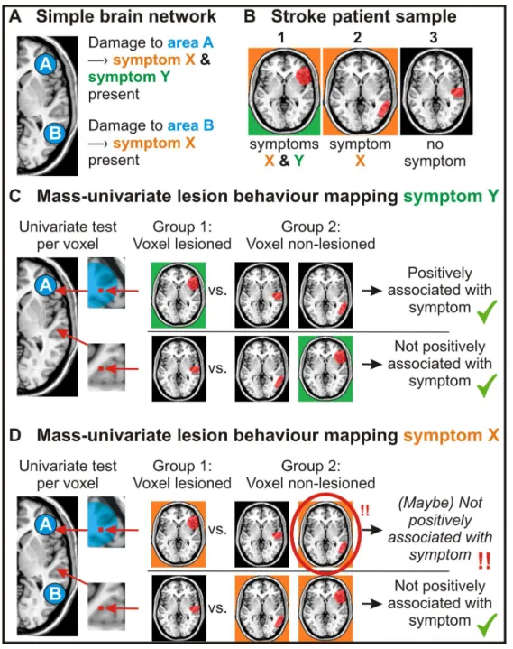
In the chapter above I elaborated on the mass-univariate nature of voxel-based lesion behaviour mapping and the independence of statistical tests. In two ways, the assumption of independence in VLBM seems to be unfitting to investigate the brain. The first is related to cognitive brain architecture. If we perform an independent statistical test on a single voxel – like in VLBM – we implicitly act as if damage to this single voxel was underlying the investigated symptom. However, lesions with the size of a single voxel (e.g. 1x1x1mm³) will most likely go clinically unnoticed. This will also happen in a voxel that was found to be associated with a symptom in a VLBM analysis. The reason is that the single voxel alone does not underlie the investigated cognitive function. Instead, neurons in many voxels have to work together to create the neural substrate of cognitive abilities. This could be a larger cluster of neurons that together form a brain region, or multiple brain regions in a brain network. In other words, neurons in a voxel work dependently with neurons in other voxels.

The independence of tests in VLBM leads to the so-called ‘partial injury problem’ (Kinkingnéhun et al., 2007; Rorden et al., 2009). A cognitive module that is

(22)

19 larger than a voxel can be damaged only partially by a lesion, i.e. some voxels of this module can be damaged and some of them remain intact. In this situation the VLBM analysis will suffer from lower power, and the analysis might fail to identify the brain module/brain network in parts or in whole. For an in-depth explanation of the partial injury problem, I’d like to refer the reader to the introduction and figure 1 of the second project of my thesis, ‘An empirical evaluation of multivariate lesion behaviour

mapping’.

3.5 The complexity of lesion anatomy

The second way in which the independence of voxel-wise statistical tests seems to be unfitting to investigate the brain is related to lesion anatomy. The cerebrum is supplied by three major brain arteries, the anterior, the middle, and the posterior cerebral artery. These arteries each supply a territory in the brain with only small overlap. These territories are located the same across humans with some variance (van der Zwan et al., 1993; Tatu et al., 2012; Neumann et al., 2016). Likewise, branches of these major arteries are – with few exceptions, especially for the anterior cerebral artery – located similarly across individuals. Thus, each branch of a major artery typically supplies a certain brain region. Further, branches of the brain arteries are differently susceptible to stroke, leading to typical locations of lesions (see Caviness et al., 2002; Sperber & Karnath, 2016). Therefore, both after ischemia and haemorrhage, brain lesions follow typical patterns along the vasculature. This fact is well illustrated by Lee at al., 2009, who show MR images of typical posterior cerebral artery stroke loci with reference to the occluded branches of the posterior cerebral artery.

Following these typical patterns, lesions often damage voxels collaterally. In other words, damage to two voxels is not independent. But how does this affect the results of VLBM? Imagine that the neural correlates of a cognitive function are organised in a small brain area A. Placed next to this brain region A is another brain region B that is not related to the cognitive function. Further imagine that both areas are supplied by the same branch of a cerebral artery. Thus, whenever the branch is occluded in stroke, both brain regions will be affected at once. Therefore, if a post-stroke cognitive symptom is present after damage to area A, area B will often be damaged as well. Likewise, if area B is damaged after stroke, most often area A will also be damaged, and the symptom is present. A VLBM analysis investigating the

(23)

20 symptom will now likely not only correctly identify area A as neural substrate of the function, but also area B. In this example, we see how the dependence of voxels in relation to stroke anatomy – from here one referred to as ‘anatomical dependence’ – can lead to wrong results in lesion behaviour mapping.

4 Investigating the validity of lesion behaviour mapping methods

In the previous chapter, I introduced a quintet of challenges and limitations present in mass-univariate lesion behaviour mapping. I discussed these points from a purely theoretical perspective, with some fictional examples. Such theoretical perspective, however, might not be sufficient in finding the optimal way to perform lesion behaviour mapping. While the multiple comparison problem does not leave much opportunity for objections, the other problems are more controversial. Especially for the last two issues – functional and anatomical dependence of voxels – there is a wide range of possible conclusions available. On the one extreme, we might now admit that some possible inaccuracies exist in lesion behaviour mapping, that we however deem to be too small or irrelevant when performing a study. On the other extreme, we might feel compelled to discard the mass-univariate entirely and abandon all findings of previous studies using this method (Mah et al., 2014; Nachev, 2015; Xu et al., 2018).

In my opinion, these problems are too complex to solve them from a purely theoretical perspective. If we aim to find out if these issues considerably affect the validity of VLBM, or if we want to find out which strategy to investigate lesion-behaviour inference is superior, we need some validation method. Unfortunately, it is not trivial to investigate the validity of lesion behaviour mapping. Ideally, the results of a lesion behaviour mapping analysis would be compared with some ground truth, i.e. a cognitive module that is anatomically well known and thus represents a gold standard. A valid analysis of the related cognitive function should then identify the ground truth. However, the knowledge we have of brain architecture is largely based on lesion behaviour mapping. Using our knowledge of the brain to define a ground truth thus is a circular error. In a review paper (Sperber & Karnath, 2018), I addressed this problem at greater length, and proposed several strategies to investigate the validity of lesion behaviour mapping methods. In my dissertation, one of these approaches plays the most important role: simulation studies.

(24)

21

4.1 A simulation approach to test the validity of lesion behaviour mapping

We can investigate the validity of lesion behaviour mapping with simulations. These simulations require a sample of real lesions, which are processed into binary, normalised lesion maps. The behavioural scores required for lesion behaviour mapping, however, are no real data. Instead, these are simulated data. The central idea is that we arbitrarily choose the anatomical ground truth underlying a cognitive function. For example, we decide that the inferior parietal gyrus – as defined by any brain atlas – is the neural correlate of a fictional symptom. Next, we compute a score for the behavioural symptom for each lesion. For example, we could decide that each lesion that has at least 10% of all voxels in the inferior parietal gyrus damaged is associated with the presence of a binary symptom. If we instead desire a continuous variable, we could choose an algorithm that computes a behavioural score from a lesion’s damage to the inferior parietal gyrus. A simple, straight-forward algorithm is a linear relation between damage to the inferior parietal gyrus and the behavioural score. In its simplest version, the behavioural score is equivalent to the damage in the region. For example, a lesion that affects 25% of all voxels in the inferior parietal gyrus would be associated with a behavioural score of 25; the maximum obtainable score would then be 100, indicating maximal symptom severity.

There are several advantages of simulation studies. First, and most importantly, we have exact knowledge about the ground truth, i.e. the anatomical correlates of a symptom. For this very reason, we can use simulations to validate lesion behaviour mapping. Second, an infinite amount of ground truth regions or simulation algorithms can be chosen. This allows us to perform large group studies with complex designs. Third, simulations provide us with a tool to investigate all the issues that I introduced in chapter 3. By using real lesions in simulations, we will likely find the usual effects of lesion size, and damage between voxels is dependent. Further, we can choose ground truths that consist of multiple regions, thus adding functional dependence between voxels. A major limitation of simulations is limited ecological validity – simulation algorithms are likely over-simplified, with real lesion-behaviour relations being more complex in several aspects. Still, such simulations provide us with a powerful opportunity to validate lesion behaviour mapping. Consequently, several studies utilised simulation approaches to compare different approaches to lesion behaviour mapping (Rorden et al., 2009; Mah et al., 2014; Inoue et al., 2014b; Zhang et al., 2014; Pustina et al., 2018; DeMarco & Turkeltaub, 2018).

(25)

22

4.2 The independence of statistical tests in the mass univariate approach put on trial

Some studies used simulations to investigate if functional or anatomical dependence between voxels affects lesion behaviour mapping. The first study came from the Nachev group (Mah et al., 2014), and was – so far – the most influential one. This study aimed to investigate if and how much VLBM is affected by functional or anatomical dependence. In a first experiment, they investigated simulations that were only based on damage to one single voxel. Thus, there was no functional dependence of voxels present, but due to the use of real lesions, anatomical dependence was. They found that maps of statistically significant voxels in a VLBM were not centred on the simulation’s ground truth voxel, but shifted by on average 16mm towards the centre of the vascular territory. In a second experiment, they investigated what happens if functional independence comes into play. They based simulations on two ground truth regions, in a way that damage to either region could lead to the simulated symptom. Doing so they showed that VLBM can yield results that can be grossly misplaced. The authors concluded that the only possible consequence was nothing less than the abandonment of mass-univariate lesion behaviour mapping in its entirety. The same position was hold in subsequent review papers by the Nachev group (Nachev, 2015; Xu et al., 2018). In parallel, the study by Inoue et al. (2014) investigated the same questions, with only slightly different simulations. Their findings mirrored the ones by Mah et al. (2014), thus strengthening their quality by a first replication.

The issues with functional independence were further disseminated in the studies by Zhang et al. (2014) and Pustina et al. (2018). They also investigated simulation ground truths consisting of multiple regions, however with a more elaborated design. Both studies found that VLBM often fails to identify all ground truth regions, and instead only correctly identifies some of them. These findings are in line with the partial injury problem (see chapter 3.4).

To sum up, some studies have shown that the assumption of independence in mass-univariate lesion behaviour mapping indeed leads to errors. This was found to be the case for both functional and anatomical independence of voxels. Although I do not fully agree with the rigorous criticism expressed by Nachev and colleagues, I think that these issues in VLBM are a clear limitation. From personal experience, I especially see problems in identifying brain networks, which is hampered by the partial injury problem. As examples where this issue is highly relevant, I see apraxia

(26)

23 of pantomime (see the third project in my thesis, ‘The network underlying human higher-order motor control: Insights from machine learning-based lesion-behaviour

mapping’) or spatial neglect (see Karnath & Rorden, 2012). For both symptoms,

VLBM studies found markedly heterogeneous results. As outlined in my review (Sperber & Karnath, 2018), this heterogeneity might have originated from the partial injury problem. VLBM analyses might have identified only parts of the underlying brain networks, and the parts found in each study might have varied due to random sampling effects or due to smaller methodological differences.

5 Multivariate lesion behaviour mapping

The findings by Mah et al. (2014) lead to vigorous discussions on the validity of mass-univariate lesion behaviour mapping, and the flames were fanned by a parallel development: the advent of multivariate lesion behaviour mapping (MLBM).

The central idea behind MLBM is to compute (statistical) models not for each voxel individually, but for multiple voxels or regions at once. Theoretically, any multivariate statistical method that can model a dependent variable (in VLBM: the behavioural score) based on multiple independent variables (in VLBM: voxel-wise lesion status) could be considered here. Methods such as multiple regression or n-way ANOVAs (for n ≥ 2), however, are limited in lesion behaviour mapping, as they are not suited to compute models based on enormous numbers of independent variables. Such methods are especially problematic if the number of observations (i.e. the number of subjects) is smaller than the number of independent variables. Thus, previous implementations of MLBM utilised more complex ways to model data. Such can be machine learning algorithms such as a support vector machine (SVM). SVMs model a binary variable based on a large number of variables (for more information see Vapnik, 1995; Hastie et al., 2008). As machine learning algorithms play an important role in my thesis, we require some technical terms: the dependent variables in machine learning are often referred to as input variables or features. The predicted variable, or target variable, can be a binary or a continuous variable. When the target variable is binary (e.g. symptoms present vs. symptom not present), the algorithms are used to perform a classification. When it is continuous, the algorithms are used to perform a regression.

(27)

24 spatial neglect (Smith et al., 2013). Aim of the study was to find a SVM that can classify patients only by using anatomical data. Such SVM model could provide new insights into lesion-deficit inference. As features, Smith et al. computed the proportion of damage to a priori chosen regions of interest. These regions of interest were taken from brain atlases. In so-called cross-validation, the performance of SVMs was assessed. It was investigated if combinations of either two or three features (i.e. damage to two or three regions of interest) provide better models than SVMs using less features, that is either one or two regions. This strategy points at a major challenge: the relevance of a single feature in SVM is difficult to access. A viable strategy is to compute a SVM on a set of features, and then remove one feature. If model performance significantly decreases, the one feature was important. The problem in MLBM is that with many features, like dozens of regions of interest or even thousands of voxels, the amount of possible feature combinations explodes. Therefore, the study by Smith et al. was restricted to a maximum of three features.

All in all, there are several disadvantages to this approach. First, it is limited to a priori chosen regions of interest. Second, although strictly speaking being multivariate, the approach is limited to a small number of features. Third, being a classification, the full variance of continuously measured behaviour cannot be investigated. These problems are shared with another multivariate approach based on game theory (Toba et al., 2017).

The next study that used MLBM was the study by Mah et al. (2014), who did not only identify problems with VLBM (see chapters 3.4 and 3.5), but additionally suggested that MLBM might be the only way to obtain valid lesion-brain inference. However, they also faced the challenge of interpreting the relevance of features in SVM. They performed a SVM on voxel level. To do so, they included the damage status of each voxel (damaged vs. not damaged) as features. With such large amount of features, a direct comparison between SVM models is not an option. Instead, they assessed the feature weights. In a SVM, each single feature is weighted in order to generate the model. This feature weighting is not informative on its own, and it does not tell us if a feature significantly contributes to a model. However, feature weights can be ranked. Mah et al. aimed to directly compare VLBM with MLBM. In the VLBM, they found a certain amount of significant voxels. Then, in the SVM, they selected the same amount of voxels, and chose the voxels that had the highest feature weight. This approach allowed a limited comparison of univariate versus multivariate

(28)

25 lesion analysis, yet it is not a practically usable approach. Importantly, Mah et al. postulated that MLBM is able to overcome the problems related to both functional and anatomical dependence of voxels. Their simulations, however, only pointed at better performance of MLBM in regard to functional dependence (see chapter 3.4), but not anatomical dependence (see chapter 3.5). Still, the authors heavily emphasized the importance of MLBM to overcome the problems related to anatomical dependence, and maintained this position in two review papers (Nachev, 2015; Xu et al., 2018).

Only shortly after the study by Mah et al. (2014), Zhang et al. (2014) published the next study that implemented MLBM. This study finally was able to overcome the problem with interpreting features. As in the MLBM approach by Mah et al., Zhang et al. included information from individual voxels as features. Instead of a SVM, they employed a support vector regression (SVR). This is an algorithm that extents SVM so that continuous target variables can be included. The major innovation was a permutation approach to test the contribution of each voxel to the SVR model. As in Mah et al., the model was computed and feature weights were assessed. Next, the same procedure was performed for a large amount of random permutations of the behavioural data. Latter analyses shows what feature weights can be expected with random data. Like commonly done in permutation testing, statistical thresholds can be inferred from these analyses to assess statistical significance of feature weights in the analysis of real data. The resulting topography is a voxel-wise map of statistical significance.

This approach, termed support vector regression based lesion symptom mapping (SVR-LSM), has several advantages. First, it is able to model continuous target variables. Second, it includes individual voxels as features, and thus it does not depend on the quality of any a priori parcellation of the brain. Furthermore, the modelling process can include an immense amount of voxels, even up to a whole brain analysis. Last but not least, the method underwent an elaborated validation by simulations. These simulations have shown that SVR-LSM outperforms VLBM in identifying complex functional modules like brain networks. In other words, SVR-LSM is able to capture the functional dependence of voxels. Likely due to these benefits, SVR-LSM was quickly adopted in the field (Mirman et al., 2015b; Fama et al., 2017; Griffis et al., 2017; Ghaleh et al., 2018; DeMarco & Turkeltaub, 2018), and I adopted this method while working on my thesis to investigate the neural correlates

(29)

26 of spatial neglect (Wiesen et al., submitted), the line bisection error, and apraxia. The latter is part of the present thesis.

Note that in recent years, more attempts to establish multivariate lesion-brain inference were made (e.g. Yourganov et al., 2015; Toba et al., 2017; Pustina et al., 2018). These approaches were not investigated or used in my thesis. Therefore, I will not further discuss them. This shall not hide the fact these methods also have potential to complement lesion-deficit inference.

6 Empirical research questions in my thesis

6.1 Impact of correction factors in human brain lesion-behavior inference

The first empirical work takes a second look at the validity of VLBM. It closely follows the work by Mah et al. (2014), who found systematic errors in VLBM due to functional and anatomical dependence of voxels. In my work, I challenge the severe criticism on VLBM by putting a focus on two correction factors in VLBM: correction for lesion size and restriction of the analysis to voxels with sufficient power. Both factors were neglected in the study by Mah et al. Using simulations, my study shows that this has inflated errors in VLBM, and that correction for lesion size is generally beneficial in VLBM.

6.2 An empirical evaluation of multivariate lesion behaviour mapping

The second empirical work examines the SVR-LSM approach. Although previous studies have shown the superiority of SVR-LSM in detecting functionally dependent brain modules, many open questions remained. A major theoretically relevant question is, if SVR-LSM not only captures functional dependence between voxels, but also anatomical dependence. Several authors advertised multivariate lesion behaviour mapping as only valid way to analyse lesion-deficit inference because it captures the anatomical dependence of voxels. However, it was never properly investigated before if MLBM indeed is able to do so. In my thesis, I use simulations to show that this in fact not the case – SVR-LSM still suffers from systematic biases due to lesion anatomy. Furthermore, I investigate the practically relevant questions if SVR-LSM requires a correction for multiple comparisons, and what sample sizes are required in SVR-LSM.

(30)

27

6.3 The network underlying human higher-order motor control: Insights from machine learning-based lesion-behaviour mapping

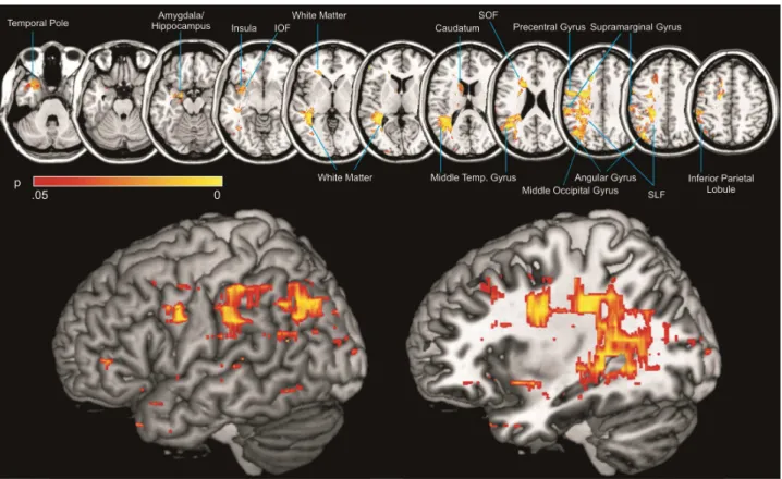
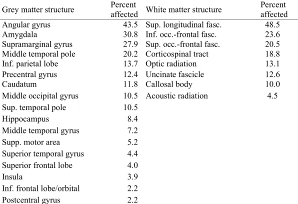
The third empirical work finally applies SVR-LSM to investigate the neural correlates of real behaviour. Here, I investigate the apraxia of pantomime. Previous studies investigated apraxia with VLBM, and their results were heterogeneous. A possible explanation might be that the actual neural correlates of apraxia are a complex brain network, where VLBM is limited due to the partial injury problem. In my thesis, I showed that SVR-LSM identifies multiple brain regions to underlie apraxia. All these brain regions were found by previous VLBM studies, but often in isolation. This suggests that SVR-LSM is a valuable tool when brain functions organised in networks are investigated.

7 Future challenges and research directions in lesion behaviour

mapping

A large amount of methodological innovations in the field of lesion-deficit inference came up in the last years. Besides MLBM, several methods based on magnetic resonance imaging also allow insights into lesion-deficit inference. Among those are fMRI, resting-state fMRI, diffusion tensor imaging, and perfusion imaging. In a review paper, I discussed how these methods can be used in neurological patients to investigate the functional anatomy of the brain (Karnath et al., 2018). For new research directions in the near future, it suggests itself to utilise these methods to study brain anatomy. Currently, I apply MLBM to gain new insights into the neural correlates of several neurological deficits. Furthermore, I would like to deepen the understanding of anatomical networks underlying praxis skills by using diffusion tensor imaging. I believe this method is better suited to identify involved white matter tracts than lesion behaviour mapping methods. In this case, lesion behaviour mapping and fibre tracking nicely complement each other.

Additionally, there are major challenges that require methodological refinement. These methodologically oriented research directions also logically follow the works in my thesis: the optimisation of MLBM and its clinical application.

7.1 Optimisation of (multivariate) lesion behaviour mapping

With the help of the simulation approach, it was shown that MLBM is superior to VLBM in some regards. Still, MLBM is far from being perfect. One main problem is