Durham E-Theses
Nonparametric Predictive Methods for Bootstrap and
Test Reproducibility
BINHIMD, SULAFAH,MOHAMMEDSALEH
How to cite:
BINHIMD, SULAFAH,MOHAMMEDSALEH (2014) Nonparametric Predictive Methods for Bootstrap and Test Reproducibility, Durham theses, Durham University. Available at Durham E-Theses Online:
http://etheses.dur.ac.uk/9493/
Use policy
The full-text may be used and/or reproduced, and given to third parties in any format or medium, without prior permission or charge, for personal research or study, educational, or not-for-prot purposes provided that:
• a full bibliographic reference is made to the original source
• alinkis made to the metadata record in Durham E-Theses
• the full-text is not changed in any way
The full-text must not be sold in any format or medium without the formal permission of the copyright holders. Please consult thefull Durham E-Theses policyfor further details.
http://etheses.dur.ac.uk
Nonparametric Predictive
Methods for Bootstrap
and Test Reproducibility
Sulafah BinHimd
A Thesis presented for the degree of
Doctor of Philosophy
Department of Mathematical Sciences
University of Durham
England
February 2014
My Father
who has been a great source of motivation and support
My Mother
for all her unlimited love and prayers
My lovely nephews and nieces for lighting up my life with their smiles
My Brothers and their wives
for all their love and best wishes throughout my life
All Family and Friends for encouraging and believing
Nonparametric Predictive Methods for Bootstrap
and Test Reproducibility
Sulafah BinHimd
Submitted for the degree of Doctor of Philosophy
February 2014
Abstract
This thesis investigates a new bootstrap method, this method is called Nonpara-metric Predictive Inference Bootstrap (NPI-B). NonparaNonpara-metric predictive inference (NPI) is a frequentist statistics approach that makes few assumptions, enabled by using lower and upper probabilities to quantify uncertainty, and explicitly focuses
on future observations. In the NPI-B method, we use a sample ofn observations to
createn+ 1 intervals and draw one future value uniformly from one interval. Then
this value is added to the data and the process is repeated, now withn+ 1
observa-tions. Repetition of this process leads to the NPI-B sample, which therefore is not taken from the actual sample, but consists of values in the whole range of possible observations, also going beyond the range of the actual sample. We explore NPI-B for data on finite intervals, real line and non negative observations, and compare it to other bootstrap methods via simulation studies which show that the NPI-B method works well as a prediction method.
The NPI method is presented for the reproducibility probability (RP) of some nonparametric tests. Recently, there has been substantial interest in the repro-ducibility probability, where not only its estimation but also its actual definition and interpretation are not uniquely determined in the classical frequentist statistics framework. The explicitly predictive nature of NPI provides a natural formulation of inferences on RP. It is used to derive lower and upper bounds of RP values (known as the NPI-RP method) but if we consider large sample sizes, the computation of
these bounds is difficult. We explore the NPI-B method to predict the RP values (they are called NPI-B-RP values) of some nonparametric tests. Reproducibility of tests is an important characteristic of the practical relevance of test outcomes.
Declaration
The work in this thesis is based on research carried out at the Department of Mathe-matical Sciences, Durham University, UK. No part of this thesis has been submitted elsewhere for any other degree or qualification and it all my own work unless refer-enced to the contrary in the text.
Copyright c 2014 by Sulafah BinHimd.
“The copyright of this thesis rests with the author. No quotations from it should be published without the author’s prior written consent and information derived from it should be acknowledged”.
Acknowledgements
First, Allah my God, I am truly grateful for the countless blessing you have bestowed on me generally and in accomplishing this thesis especially.
My main appreciation and thanks goes to my supervisor Prof. Frank Coolen for his unlimited support, expert advice and guidance. It is very hard to find the words to express my gratitude and appreciation for him.
My special thanks go to my friends Tahani Maturi and Zakia Kalantan for all their support and help.
I would like also to thank my examiners Dr. Matthias Troffaes and Dr. Malcolm Farrow for their useful discussions.
Thanks to Durham University, King AbdulAziz University, Jeddah, Saudi Ara-bia, and Dr. Abeer for the facilities that have enabled me to study smoothly.
My final thanks go to everyone who has assisted me, stood by me or contributed to my educational progress in any way.
Sulafah Binhimd, Durham, UK First Submit: September 2013 Viva: November 2013
Final Submit: February 2014
Contents
Abstract iii Declaration v Acknowledgements vi 1 Introduction 1 1.1 Overview . . . 11.2 Nonparametric Predictive Inference (NPI) . . . 2
1.3 Bootstrapping . . . 6
1.3.1 Efron’s Bootstrap . . . 6
1.3.2 Bayesian Bootstrap . . . 11
1.3.3 Banks’ Bootstrap . . . 12
1.3.4 Comparison of Bootstrap Methods . . . 13
1.4 Reproducibility . . . 17
1.5 Outline of Thesis . . . 22
2 NPI Bootstrap 24 2.1 Introduction . . . 24
2.2 The General Idea of NPI Bootstrap . . . 25
2.3 NPI Bootstrap for Finite Intervals . . . 28
2.4 NPI Bootstrap on Real Line . . . 35
2.5 Comparison With Other Methods . . . 43
2.5.1 Confidence Intervals . . . 43
2.5.2 Prediction Intervals . . . 46 vii
2.6 NPI-B for Order Statistics . . . 60
2.7 Concluding Remarks . . . 62
3 NPI for Reproducibility of Basic Tests 64 3.1 Introduction . . . 64
3.2 Overview of Some Basic Tests . . . 65
3.2.1 One Sample Sign Test . . . 65
3.2.2 One Sample Signed Rank Test . . . 66
3.2.3 Two Sample Rank Sum Test . . . 67
3.3 NPI for the Reproducibility Probability . . . 69
3.4 NPI-RP for the One Sample Sign Test . . . 72
3.5 NPI-RP for the One Sample Signed Rank Test . . . 82
3.6 NPI-RP for the Two Sample Rank Sum Test . . . 92
3.7 Concluding Remarks . . . 101
4 Reproducibility using NPI-Bootstrap 104 4.1 Introduction . . . 104
4.2 NPI-B-RP for the One Sample Sign Test . . . 105
4.3 NPI-B-RP for the One Sample Signed Rank Test . . . 113
4.4 NPI-B-RP for the Two Sample Rank Sum Test . . . 116
4.5 NPI-B-RP for the Two Sample Kolmogorov Smirnov Test . . . 120
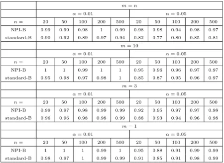
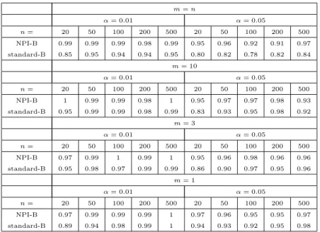
4.6 Performance of NPI-B-RP . . . 122
4.6.1 Mean Square Error with NPI-B-RP . . . 122
4.6.2 Predictive Performance of NPI-B-RP . . . 125
4.7 Concluding Remarks . . . 128
5 Conclusions 129
Chapter 1
Introduction
1.1
Overview
Recently nonparametric predictive inference (NPI) [6, 17, 19] has been developed as a frequentist statistical approach that uses few assumptions. It uses lower and upper probabilities for events of interest considering future observations, and is based
on Hill’s assumption A(n) [45–47]. The lower and upper probabilities of NPI are
introduced by Coolen and Augustin [6], they showed that NPI has strong consistency properties in the theory of interval probability [25, 68].
The standard bootstrap (standard-B) was introduced by Efron [35]. It is a resam-pling method for statistical inference, and a computer based method for assigning measures of accuracy to statistical estimates. Thereafter, various versions of boot-strap were developed such as smoothed Bayesian bootboot-strap, which was developed by Banks’ [8].
In this thesis we present the NPI bootstrap method, which we indicate by NPI-B, as an alternative to other well known bootstrap methods, and then we discuss its performance, and use it to predict the reproducibility probability (RP). The reproducibility probability is a helpful indicator of the reliability of the results of statistical tests. The predictive nature of NPI provides a natural formulation of inference on reproducibility probability which is an important characteristic of sta-tistical test outcomes. In this thesis we consider RP within a frequentist stasta-tistical framework but from the perspective of prediction instead of estimation.
Section 1.2 presents a brief introduction to NPI. In Section 1.3 we describe various bootstrap methods and Section 1.4 reviews the reproducibility probability for tests. The outline of this thesis is provided in Section 1.5.
1.2
Nonparametric Predictive Inference (NPI)
In classical probability, a single (precise) probability P(A) is used for each event
A but if the information is vague, the “imprecise probability” is an alternative
ap-proach which uses an interval probability instead of single probability P(A). The
interval probability is specified by lower and upper probabilities and denoted by
P(A) and P(A), respectively, where 0≤P(A)≤P(A)≤1, [25].
Nonparametric predictive inference (NPI) [6, 17, 19] is a statistical technique based on Hill’s assumption A(n). Hill [45] introduced the assumption A(n) for
pre-diction if there is no prior information about an underlying distribution. It is used
to predict direct conditional probabilities for one future valueYn+1 or more than one
future value Yi, i ≥ n+ 1. Conditional on the observed values, the n+ 1 intervals
are created by n ordered, exchangeable and continuous random quantities on the
real line y(1) < y(2) < ... < y(n), assigned equal probabilities for the next
obser-vation to belong to each of these intervals, which are denoted by I1 = (−∞, y(1)),
Il = (y(l−1), y(l)), for l = 1,2, ..., n+ 1, and In+1 = (y(n),∞). The assumption A(n)
is:
P(Yn+1 ∈Il) =
1
n+ 1 (1.1)
for l = 1,2, ..., n+ 1. Hill gave more details about A(n) in [46] and [47]. It is clear
that A(n) is a post data assumption and the statistical inferences based on it are
predictive and nonparametric, and it is suitable if there is no knowledge about the random quantity of interest. A(n) is not sufficient to get precise probabilities for any
event of interest, but it does give bounds (lower and upper) for probabilities which are called “interval (valued) probabilities” or “imprecise probabilities”. They are lower and upper probabilities in interval probability theory [19, 68].
1.2. Nonparametric Predictive Inference (NPI) 3
Coolen [15] gave an example to explain the dependence of Y related to A(n):
Suppose we have a single observation y1, providing two intervals, I1, I2. The
as-sumptionA(1) now states thatP(Yi ∈I1) =P(Yi < y1) = n+11 = 12 for all i≥2. Let
us considerY3, and in particular how probability statements about Y3 change when
learning the value ofY2. If we remain interested in the eventY3 < y1, the probability
P(Y3 < y1) = 12 will change, assumingA(2), according to whether the value ofY2 will
be less than or greater thany1, P(Y3 < y1|Y2 < y1) = 32 or P(Y3 < y1|Y2 > y1) = 13,
respectively. This is related to the probabilityP(Y3 < y1) = 12 without conditioning
on the unknownY2 by the theorem of total probability,
P(Y3 < y1) =P(Y3 < y1|Y2 < y1)P(Y2 < y1) +P(Y3 < y1|Y2 > y1)P(Y2 > y1) = (23 ×1 2) + ( 1 3 × 1 2) = 1 2
A direct consequence of A(2) is that these probabilities for Y3 keep the same values
if the unknown Y2 is replaced by its observed value y2, so P(Y3 < y1|y2 < y1) = 23
and P(Y3 < y1|y2 > y1) = 13.
Augustin and Coolen [6] referred to the statistical approach known as
nonpara-metric predictive inference (NPI) based on A(n). They introduced the lower and
upper probabilities of NPI, and explained that NPI based only on theA(n)
assump-tion has strong consistency properties in the theory of interval probability [25, 68]. NPI is exactly calibrated [53], which is a strong consistency property in the fre-quentist theory of statistics, and it never leads to results that are in conflict with inferences based on empirical probabilities.
The lower probability for an event A is denoted by P(A) and the upper
proba-bility byP(A). The lower probability in NPI is the maximum lower bound for the
classical (precise) probability for A, P(A), and the upper probability in NPI is the
minimum upper bound forA, whereP(A)∈[0,1]. The classical (precise) probability
is a special case of imprecise probability whenP(A) =P(A) , 0≤P(A)≤P(A)≤1,
whereasP(A) = 0 andP(A) = 1 represent an absence of information aboutA. The
NPI lower and upper probabilities for the eventYn+1 ∈B where B ⊂R are :
P(Yn+1 ∈B) = 1 n+ 1|{l :Il ⊆B}| (1.2) P(Yn+1 ∈B) = 1 n+ 1|{l :Il \ B 6=∅}| (1.3)
The lower probability (1.2) is the total taking only probability mass into account
that must be in B, which is only the case for the probability mass n+11 per interval
Il, if this interval is completely contained within B. The upper probability (1.3) is
the total of all the probability mass into account that can be inB, which is the case
for the probability mass n+11 , per interval Il, if the intersection of Il and B is non
empty.
NPI is used in a variety of statistical fields such as quality control [4, 5] and precedence testing [28]. The NPI method was explained in statistical process control by Arts, Coolen and van der Laan [5] who presented extrema charts and the run length distribution for these charts via simulation examples and compared them with other types of charts. Coolen and Coolen-Schrijner [21] used lower and upper probabilities for predictive comparison of different groups of proportions data. They considered NPI pair wise comparison of groups and then generalized to multiple comparisons. To illustrate their method and discuss the features, they analyzed two data sets and explained the importance of the choice of the number of future trials, then analyzed the imprecision in their results. Maturi et al [57] compared the failure times of units from different groups in life testing experiments if each unit failed at most once, and studied the effect of the early termination of the experiment on the lower and upper probabilities.
For data sets containing right-censored observations, Coolen and Yan [24] devel-oped ’right censoring A(n)’ which is a generalization of A(n). Coolen-Schrijner and
Coolen [27] used that generalization to find a method for the age replacement of tech-nical units, and in simulations they found this method performed well. Coolen [17] explained NPI for circular data and multinomial data to show that it is possible to apply NPI to different data situations. He described two norms of objective Bayesianism, which both have a predictive nature.
The NPI approach is also used with multinomial data [7] when the observations fall into one of several unordered categories. It considers whether the number of categories is known or unknown. In the same paper the same idea is illustrated to deal with sub-categories, where it is assumed that the main category divides into several not overlapping sub-categories. In all cases, the multinomial data are
1.2. Nonparametric Predictive Inference (NPI) 5
represented as observations on a probability wheel, like circular data. Recently presented NPI methods for statistical inference and decision support considered, for example, precedence testing [28], accuracy of diagnostic tests [26,39] and acceptance decisions [22, 40]. In Chapter 3, we apply NPI to Bernoulli data [16] and to multiple real valued future observations [5].
NPI for Bernoulli random quantities [16] is based on a latent variable represen-tation of Bernoulli data as real-valued outcomes of an experiment, in which there is a completely unknown threshold value, such that the outcomes on one side of the
threshold are successes and on the other side are failures. The use ofA(n) together
with lower and upper probabilities enables inference without a prior distribution on the unobservable threshold value, as is needed in Bayesian statistics where this threshold value is typically represented by a parameter.
Assume that there is a sequence of n+m exchangeable Bernoulli trials, that
’success’ and ’failure’ are possible outcomes of each one of these trials, and that
the data consisting of s successes in n trials. Let Yn
1 denote the random number
of successes in trials 1 to n, then a sufficient representation of the data for NPI
is Yn
1 = s, due to the assumed exchangeability of all trials. Let Ynn+1+m denote
the random number of successes in trials n+ 1 to n+m, or in future trials. Let
Rt = {r1, . . . , rt}, with 1 ≤ t ≤ m+ 1 and 0 ≤ r1 < r2 < . . . < rt ≤ m, and, for
ease of notation, define s+r0
s
= 0. Then the NPI upper probability for the event
Ynn+1+m ∈Rt, given dataY1n=s, fors ∈ {0, . . . , n}, is
P(Ynn+1+m ∈Rt|Y1n=s) = n+m n −1 t X j=1 s+rj s − s+rj−1 s n−s+m−rj n−s (1.4)
The corresponding NPI lower probability can be derived via the conjugacy property
P(Ynn+1+m ∈Rt|Y1n=s) = 1−P(Ynn+1+m ∈Rct|Y1n =s) (1.5)
whereRc
These NPI lower and upper probabilities are the maximum lower bound and minimum upper bound, respectively, for the probability for the given event based on
the data, the assumptionA(n) and the model presented by Coolen [16]. In Chapter
3 an explanation of the derivation of these NPI lower and upper probabilities is given, using a counting argument of paths on a grid. This is included in order to provide a combinatorial argument to prove an important claim in Section 3.4.
1.3
Bootstrapping
In this section we present a description of different bootstrap methods, some of them are used in this thesis, such as Efron’s bootstrap and Banks’ bootstrap.
1.3.1
Efron’s Bootstrap
The bootstrap method was introduced by Efron [35]. It is a resampling technique for estimating the distribution of statistics based on independent observations, then developed to work with other statistical inferences. It is used for assigning the measures of accuracy of the sample estimate, especially the standard error. Using the bootstrap method to estimate the standard error does not require theoretical calculations, and it is available for any estimator. It is also a useful method when the sample size is not sufficient for statistical inference. The basic bootstrap method uses Monte Carlo sampling to generate an empirical estimate of the sampling distribution of the statistic (bootstrap distribution). That means it uses a plug-in principle to approximate the sampling distribution by using a bootstrap distribution. In most cases a bootstrap distribution mimics the shape, spread and bias of the actual sampling distribution. Monte Carlo sampling builds on drawing a large number of samples from the observations and finding the statistic for each sample. The relative frequency distribution of these statistics is an estimate of the sampling distribution of the statistic.
Efron [38] defined a bootstrap samplex∗ = (x∗1, x∗2, ..., x∗n). It is obtained by
ran-domly sampling n times with replacement, from the original sample x1, x2, ..., xn.
sam-1.3. Bootstrapping 7
ple. There are many references that show the principles and validity of bootstrap and how it works. Efron and Tibshirani [38] and Davison and Hinkley [31] have described bootstrap methods fully with examples and basic theories of applications, such as tests, confidence intervals and regression. Both books contain S-plus pro-grams to implement this method. Efron and Gong [37] covered the nonparametric estimation of statistical errors, especially the bias and standard error of an estima-tor, in some resampling methods such as bootstrap, jackknife and cross validation. Efron [36] was concerned with the same basics but with more efficient computational methods for bootstrap and one sample problems.
Good [42] provided a brief review of bootstrap and computer code in various software packages (c++, SAS, MatLab, R, S-plus) in order to put this method into practice. Furthermore, Hjorth [48] explored FORTRAN code, but with more studies about bootstrap.
Chernick [13] discussed the key ideas and applications of bootstrap. Also he illustrated confidence intervals, hypothesis tests, regression models and time series. Singh [66] examined the convergence of the bootstrap approximation in some cases of estimation, and considered some of the theorems with proofs. Young [70] re-viewed research into bootstrap and related methods, and additionally discussed the bootstrap of independent and dependent data.
We have the observationsx1, x2, ..., xn of independent and identically distributed
random variablesX1, X2, ..., Xn with distribution function F, and want to estimate
the parameter of interestθ, which is a function ofX, by statisticTn. Now we would
like to know the sampling distribution of the statisticTn. To do this, we will use the
bootstrap method, the main advantage of the bootstrap is that it can be applied to any statistic. There are two types of bootstrap: parametric and nonparametric bootstrap. The first type is the parametric bootstrap, which is used when we know
the exact distribution function F (or the parametric form of the population
distri-bution ), or can assume it with some knowledge about the underlying population, and then estimate the parameters. The second type is the nonparametric bootstrap,
which is used if F is completely unknown. This type is based on simulation of data
probability distribution giving a probability 1n to each value of the observations. The empirical distribution function is the maximum likelihood estimator of the popula-tion distribupopula-tion funcpopula-tion when there are no parametric assumppopula-tions. Here we show the basic steps of the nonparametric bootstrap, because it is the general method:
1. Construct Fn, the empirical probability distribution by putting probability n1
to each value x1, x2, ..., xn, Fn(x) = Pni=1I(xi ≤x)/n. It is the number of
elements which are less than or equal to xin the sample divided by size of this
sample.
2. DrawB random samples of sizen fromFn with replacement (from the original
sample which is treated as a population).
3. Calculate the statistic of interest Tn from each sample to get Tn∗1, Tn∗2, ..., TnB∗ .
4. Construct the empirical distribution ofTn∗1, Tn∗2, ..., TnB∗ by placing probability
1
B at each one of them. This distribution is a Monte Carlo approximation to
the bootstrap estimate of the sampling distribution of the statistic Tn. It is
used to make inferences about θ.
There are some possible modifications to this bootstrap procedure. Young [70] and Bickel and Freedman [10] explained a possibility of variation of the size of the data points and the size of the bootstrap sample.
The sampling distribution of a statistic shows the variation in the statistic, be-cause the statistic will vary from one sample to another. If we use the bootstrap distribution as an approximation of a sampling distribution, we have another source of variation because we resample from the original sample. To solve this problem, we should use a large original sample and draw large numbers of bootstrap samples. To estimate the accuracy of an estimator Tn, the standard error of Tn, seF (Tn), is
calculated. The bootstrap estimate ofseF(Tn) is seFn(T
∗
n). It is a plug-in estimate
because it uses the empirical distribution function Fn instead of the unknown
dis-tribution F. seFn(T
∗
n) is called the ideal bootstrap estimate of the standard error
if B → ∞, see [38], “idea” does not mean perfect. It simply refers to the use of an
infinite number of bootstrap samples. To approximate seFn(T
∗
1.3. Bootstrapping 9
Carlo approximation of the bootstrap estimate of the standard errorsedB by follow
the next algorithm:
1. DrawB random samples of size n with replacement from the empirical
distri-bution function Fn.
2. Calculate the statistic of interest Tn for each bootstrap sample to get
Tn∗1, Tn∗2, ..., TnB∗ .
3. Estimate the standard error by the sample standard deviation of the Tnj,
j = 1,2, ..., B d seB = " PB j=1 T ∗ nj−T ∗ n(.) 2 B−1 #0.5 (1.6) where Tn∗(.) = PB j=1T ∗ nj B .
Note that limB→∞dseB =seFn(Tn). So if B is very large, the difference between the
bootstrap estimate and the Monte Carlo approximation will disappear. We use the bootstrap estimate of the standard error to compare between different bootstrap methods in Chapter 2.
The main advantage of the bootstrap method is that it enables us to estimate the standard error for any estimator. We discussed the standard error as a measure
of accuracy for an estimator Tn, but there are other useful measures of statistical
accuracy like bias, which is in general the difference between the expectation of an
estimator Tn and the quantity θ being estimated,
bias(Tn, θ) =biasF =E(Tn)−θ (1.7)
Of course we want an estimator which has good characteristics such as small bias and small standard error. The bootstrap estimate of bias is
biasFn =E(T ∗ n)−T o n (1.8) where To
n is the observed value of a statistic which is calculated from the original
sample. Moreover,biasFn is the ideal bootstrap estimate of bias. It is approximated
by Monte Carlo simulation by generating independent bootstrap samples and
Tn∗(.) =
PB j=1Tnj∗
B to get the bootstrap estimate of bias based on B replications:
\
biasB =Tn∗(.)−T o
n (1.9)
If the ratio of bias to the standard error is small, we do not have to worry about bias. There is a better method than (1.9), see [38]. Let P∗ = (P1∗, P2∗, ..., Pn∗) be a
resampling vector which contains the proportion of a bootstrap samplex∗
Pb∗ = #(x
∗
i =xb)
n , b = 1,2, ..., n (1.10)
This vector satisfies 0 ≤ Pb∗ ≤ 1 and Pn
b=1P ∗
b = 1. For example, if the bootstrap
sample is x∗ = (x1, x6, x6, x5, x1, x1), then the corresponding resampling vector is
P∗ = (3/6,0,0,0,1/6,2/6). If the B bootstrap samples x∗1, x∗2, ..., x∗B give B
re-sampling vectors P∗1, P∗2, ..., P∗B, and P∗ is the average of these vectors, then the better bootstrap bias estimate is
biasB =Tn∗(.)−Tn(P∗) (1.11) where isP∗ = PB j=1P ∗ j B andTn(P
∗) is the bootstrap statistic but written as a function
of the average of the resampling vector. BothbiasB and \biasB converge tobiasFn =
d
bias∞, the ideal bootstrap estimate of bias, asB → ∞, but the convergence is faster
tobiasB. Efron and Tibshirani [38] calculated, for some data, biasB and \biasB for
B = 25,50,100, ...,3200, and biasd∞ approximated by biasd100,000, then they found biasB converged to biasd∞ more quickly.
The root mean square error of an estimator Tn for θ is a measure of accuracy
that uses both bias and standard error [38]
√
M SE=pse(Tn)2+bias(Tn, θ)2 (1.12)
Note that these procedures to find the bootstrap estimate of standard error and bias can be used in parametric and nonparametric bootstrap. In this thesis we use bias, variance, standard error and mean square error to compare different methods of bootstrap in Chapter 2.
1.3. Bootstrapping 11
Now, we should ask an important question, how large should we take B, the
number of bootstrap replications? Efron [38] made some suggestions based on his
experience. He considered that B = 50 replications is sufficient to estimate the
standard error, but B = 200 replications or more is rarely needed to estimate
a standard error. For confidence intervals and hypotheses tests B = 50 or 200
is not large enough. At least B = 1000 or 2000 replications is needed to give
accurate results. Some researchers use even larger numbers but this consumes a lot of computer time, depending on the complexity of the method. In this thesis we use
B = 1000 replications which we think is a suitable selection for our purposes here.
It is the most widely used in the literature, especially for hypothesis tests and the construction of confidence intervals, and for the regression models.
1.3.2
Bayesian Bootstrap
The Bayesian bootstrap was developed by Rubin [63]. He explained that the
Bayesian bootstrap simulates the posterior distribution of the parameter, whereas the standard bootstrap simulates the estimated sampling distribution of a statistic of the parameter. He used a noninformative prior distribution which is the uniform distribution. The standard and Bayesian bootstrap differ in how to assign the prob-abilities. In Bayesian bootstrap [13, 63], instead of sampling with replacement from
the data and with probability 1
n, it uses a posterior probability distribution for the
data. To simulate the posterior distribution of the parameter Rubin [63] used the
statistic as a function of probabilitiesg. For simplicity we will consider the data as
one dimensional and as a single parameter but both can be multidimensional. He drew n−1 random variables from uniform (0,1) to get u1, u2, ..., un−1 and ordered
them to have gaps g between these values. The vector g is the vector of
proba-bilities of the data value x1, x2, ..., xn. Then he drew a sample from the data and
found the statistic of interest as a function of g. When he repeated this process
the posterior distribution of the parameter was found. The Bayesian bootstrap can
be used in the usual Bayesian inferences about the parameterθ, which is based on
the estimated posterior distribution, but the nonparametric bootstrap just makes frequentist analysis about the distribution of statistic Tn.
Several studies have used and discussed the Bayesian bootstrap, such as Meeden [58], who presented Rubin’s Bayesian bootstrap with a new modification. He used the same argument of the Bayesian bootstrap to estimate population quantiles but applied it to subintervals divided to grid, more than one grid is used, and these grids are given and fixed. Then Meeden compared the Bayesian bootstrap and the smoothed Bayesian bootstrap to his technique to show that these three methods are quite similar and preferable to traditional methods.
1.3.3
Banks’ Bootstrap
Banks’ [8] described new versions of the bootstrap, the smoothed Efron’s bootstrap and the smoothed Bayesian bootstrap, and compared them to the Bayesian boot-strap and other bootboot-strap methods. Here we will focus on the smoothed Efron’s bootstrap. In this method Banks’ [8] smooths Efron’s bootstrap by linear inter-polation histospline smoothing between the jump points of empirical distribution. Histospline is a smooth density estimate based only on the information in a his-togram. This procedure is as follows:
1. Takenobservations, which are real valued, one dimensional on a finite interval.
2. Create n+ 1 intervals between the n observations x0, x1, x2, ..., xn, xn+1 where
x0 and xn+1 are the end points of the possible data range (finite).
3. Put uniformly distributed probabilities 1/(n+ 1) over each interval.
4. Sample n observations from the distribution.
5. Find the statistic of interest.
6. Repeat steps 4 and 5 B times to get B bootstrap samples.
In smoothed Efron’s bootstrap, the empirical distribution function Fn(x) is
smoothed using linear interpolation histospline smoothing between the jump points.
It spreads the probability 1/(n+ 1) uniformly over any interval between two values
of observations. Banks’ [8] used confidence regions to compare his method to other
1.3. Bootstrapping 13
and applied the chi-square test of goodness of fit to compare methods. The best
region is one with small volume with α (Type I error ).
1.3.4
Comparison of Bootstrap Methods
Efron [35, 37, 38] discussed different ways of comparing bootstrap methods like bias, standard error and mean square error, which are shown in Section 1.3.1. In this section, we illustrate other ways of comparison between bootstrap methods such as confidence intervals and prediction intervals.
1. Confidence Intervals
In this part we describe different methods for constructing confidence intervals by bootstrap technique. But we will start with a review of general confidence intervals.
In one sample case, we have the observations x1, x2, ..., xn with the distribution
functionF, θ is the parameter of interest with its estimationTn, seb is the estimate
of the standard error ofTn = ˆθ. In some cases, if the sample sizen grows large, the
distribution ofTn is approximated by normal with mean θ and variance (sec2), that
meansTn∼N(θ,(sec2)) or equivalently
ˆ
θ−θ b
se ∼N(0,1) (1.13)
This result is called the large sample theory or asymptotic theory. Letz(α) be the 100.αth percentile point of N(0,1), then from (1.13)
P(z(α) ≤ θˆ−θ b se ≤z (1−α)) = 1−2α (1.14) and P(ˆθ−z(1−α).se < θ <b θˆ−z(α).seb) = 1−2α (1.15)
It is called the standard confidence interval with coverage probability 1−2α, or
confidence level 100.(1−2α)%.
Now we want to explore the use of the bootstrap method to construct confidence
intervals [38], the first approach is the bootstrap-t interval. We generateBbootstrap
samples and for each one we find
Z∗(b) = ˆ θ∗(b)−θˆ \ se∗B(b) = T ∗ nj−Tn \ se∗B(b) (1.16)
where ˆθ∗(b) is the value of ˆθ of the bootstrap samplex∗b andse\∗
B(b) is the estimated
standard error of ˆθ∗ of the bootstrap samplex∗b. The bootstrap-t confidence interval
is:
(ˆθ−ˆt(1−α).
d
seB,θˆ−ˆt(α).sedB) (1.17)
where ˆt(α) is the αth percentile of Z∗(b), across all bootstrap samples b, and ˆt(1−α)
is the (1−α)th percentile. If B = 1000 and α= 0.05, then ˆt(α) is the 50th largest
value of the Z∗(b). If B.α is not an integer, assuming α ≤0.5, let k= [(B+ 1)α] is
the largest integer≤(B+ 1)α, then determine α and (1−α) by thekth largest and
(B + 1−k)th largest value of Z∗(b), respectively.
Another approach of confidence intervals using the bootstrap technique is based on the percentiles of the bootstrap distribution of a statistic. It is called the
per-centile interval. The approximate (1−2α) percentile interval is defined by :
ˆ
θ∗B(α)< θ <θˆB∗(1−α) (1.18)
Tnj∗(α)< θ < Tnj∗(1−α) (1.19) where Tnj∗(α) is the 100.αth empirical percentile of the Tnj∗ values and Tnj∗(1−α) is
the 100.(1−α)th empirical percentile of them, that means the B.αth value and
B.(1−α)th value of the ordered list of the B replications of Tn∗. For example, if
B = 1000 andα= 0.05, Tnj∗(α) and Tnj∗(1−α) are the 50th and 950th ordered values of the replications, respectively.
The percentile interval can be improved to get a BCa interval, or a bias corrected
and accelerated interval. To find the endpoints which are given by percentiles,
we need to compute two numbers ˆa and ˆz0, they are called the acceleration and
bias correction, respectively. The value of the bias correction ˆz0 uses the ratio of
bootstrap replications less than the original estimateTn, it counts the possible bias
inTn as an estimate of θ
ˆ
z0 = Φ−1(
#(Tnj∗ < Tn)
B ) (1.20)
where Φ−1 is the inverse function of a standard normal cumulative function, for
1.3. Bootstrapping 15
by jackknife values of a statistic Tn. Let xi = (x1, x2, ..., xi−1, xi+1, ..., xn) be the
jackknife sample which is the original sample with the ith observation xi deleted,
Tn(i) is the i−th jackknife replication of Tn and
Tn(.) = Pn i=1Tn(i) n (1.21) then ˆ a= Pn i=1(Tn(.)−Tn(i)) 3 6(Pn i=1(Tn(.)−Tn(i))2) 3 2 (1.22)
It refers to the rate of change of the standard error ofTn asθ varies.
The (1−2α) BCa interval in [38] and [56] is:
Tnj∗(α1) < θ < Tnj∗(α2) (1.23) where α1 = Φ(ˆz0 + ˆ z0+zα 1−ˆa(ˆz0+zα) ) (1.24) α2 = Φ(ˆz0+ ˆ z0+z1−α 1−ˆa(ˆz0+z1−α) ) (1.25)
Φ(.) is the standard normal cumulative function and z(α) is the 100.αth percentile
point of standard normal distribution. For example,z(0.95) = 1.645 and Φ(1.645) =
0.95. If ˆa and ˆz0 equal zero, then α1 = Φ(z(α)) = α, α2 = Φ(z(1−α)) = 1−α, and
the BCa interval and percentile interval are equal in this case.
We will use the BCa interval in Section 2.5.1 to compare different bootstrap methods because it has a higher order of accuracy and transformation respecting. To illustrate the transformation respecting property we consider an example, if we
constructed a confidence interval for a parameter θ, then the interval for θ2 will
construct by squares the end points of confidence interval for θ, this interval that is
transformation respecting [38].
2.Prediction Intervals
In [55], the bootstrap method was used to construct a prediction interval for one or more future values from the Birnbaum-Saunders distribution. They applied the bootstrap percentile method with the bootstrap calibration for estimating the
Birnbaum Saunders distribution functionF with parametersα, β. A bootstrap sam-ple of size n, x∗1, ..., x∗n, is drawn from x1, ..., xn with replacement to construct the
estimated distributionF∗, and then sampledy∗1, ..., ym∗ from it, (m is the number of future observations), we can obtain the mean of y1∗, ..., y∗m, which is denoted by ¯y∗m. Repeat this technique B times to get B values of ¯ym∗, denoted by ¯ym∗(1), ...,y¯∗m(B).
The 1−αprediction interval for ¯xm (the mean of future observations in the
popula-tion) is: [¯y∗( α 2) m,B,y¯ ∗(1−α 2)
m,B ]. The lower bound ¯y
∗(α2)
m,B is theB.
α
2th value in the ordered list
of the B replications of ¯ym∗, and the upper bound ¯y∗(1−
α
2)
m,B is the B.(1−
α
2)th value
in the same ordered list. To find the coverage count how many intervals contain ¯
xm. This procedure is used to predict one or more future observations. To explain
this, for example, if we have a sample of x1, x2, x3 , n = 3, and want to predict
m = 3 values, x4, x5, x6, the mean of these values is ¯xm = ¯x3. Then we construct
the prediction interval for it by sampling the bootstrap sample x∗1, x∗2, x∗3 and then generating from themy1∗, y∗2, y∗3 and finding ¯y∗m. Repeat thisB = 1000 times and find
the prediction interval of theseB values as described before. If we consider the case
of prediction of one future valuex4 the mean will not be used here. Simply resample
x∗1, x∗2, x∗3 and generate y∗1 from them, and repeat this B times to have the list of
B values y1∗(1), y1∗(2), ..., y1∗(B) to construct the prediction interval for xn+1 = x4.
In that study, the 90% and 95% prediction intervals for a single future value xn+1
and the mean ofmfuture observations ¯xmare obtained, and MonteCarlo simulation
is used to estimate the coverage probability by finding the proportion of intervals which contain xn+1 and ¯xm.
Different types of bootstrap prediction intervals [2,60,61] can be used to estimate
the parameterθ: bootstrap-t, percentile and BCa prediction intervals. In this thesis
we use the percentile prediction interval. Let X = (X1, X2, ..., Xn) be the past
random samples and Y1, Y2, ..., Ym be the future random samples, where X and Y
are iid from probability distributionF andT = ˆθis a scalar parameter, and we want
to construct the prediction interval to predict the statistic (estimator) of θcm =Tm
of the future random sample. Let θbn = Tn be the estimator using the past sample
of sizen. Fn and Fm are the CDF ofTn and Tm, respectively, and let ˆFn and ˆFm be
1.4. Reproducibility 17 1
m on each Y
∗
i . The (1−2α)% percentile prediction interval
lower bound = ˆFm−1[Φ(z(α)(1 + m n) 1 2)] = ˆF−1 m [α1] (1.26) here,r = mn and z(α) = Φ−1(α) upper bound = ˆFm−1[Φ(z(1−α)(1 + m n) 1 2)] = ˆF−1 m [α1] (1.27)
In [61]X∗ andY∗ are drawn from the past sampleXwith replacement while [60] the
iterated (calibration) bootstrap was used by generatingX∗andY∗ fromXand then
resampleY∗∗fromX∗, to study the improving of the coverage accuracy of prediction
intervals. The percentile prediction interval to predict future observations, and the percentile prediction interval to predict the statistic, are used in Section 2.5.2 to compare the NPI-B method with the standard-B method.
1.4
Reproducibility
Often when we use the applications of the statistical test in several fields, we meet some problems because the results and conclusions of statistical hypothesis tests can be different each time the tests are repeated. Goodman [43] raised the topic of re-producibility of a statistical test, mainly to counter a frequently occurring
misunder-standing about the meaning of a statisticalp-value. The reproducibility probability
(RP) for a test is the probability for the event that, if the test is repeated based on an experiment performed in the same way as the original experiment, the test outcome, that is either rejection of the null-hypothesis or not, will be the same. The focus is mostly on reproducibility of tests in which the null-hypothesis is rejected, as signifi-cant effects tend to lead to new treatments in medical applications, for example. In a later discussion of Goodman’s paper (and about twice the length of Goodman’s
paper), Senn [64] emphasized the different nature of thep-value and RP. Senn agrees
with Goodman about the importance of reproducibility of test results and the RP,
but disagrees with Goodman’s claim that ‘p-values overstate the evidence against
the null-hypothesis’. Indeed, it is important to recognize the difference between RP
and the p-value, while also recognizing a natural link between the two, in the sense
p-value in the case of a rejected null-hypothesis, the larger one would expect the corresponding RP to be.
Senn [64] also discusses the importance of reproducibility of tests in the real world, where actual repeats of tests may well be under slightly different circum-stances and might involve different teams of analysts performing the tests. So, the concept of reproducibility is not necessarily uniquely defined, and statistical method-ology should be flexible enough to deal with varying circumstances. Recently, Begley and Ellis [9] presented a worrying insight into problems with reproducing tests in preclinical cancer research in which significant effects were reported. Attempting to repeat tests from 53 ‘landmark studies’, they managed to get the same significant scientific findings in only 6 cases. They report further on similar, but more extensive, studies by Bayer Healthcare in Germany, where only about 25 percent of significant results had been reproduced. Begley and Ellis [9] provide a detailed discussion of factors that play a role in such studies of repeatability and provide guidelines for improving the reliability of such studies which, for example, considers publication processes (there is an obvious bias due to the tendency for only ‘positive’ results to be published). Remarkably, Begley and Ellis [9] do not discuss the statistical methods used in such medical testing, where more emphasis on RP seems a natural requirement as part of a solution for more reliable medical testing.
During the last decade, the concept of RP has attracted increasing interest in the literature, with some contributions making clear that the definition and interpreta-tion of RP are not uniquely determined. Miller [59] emphasizes that two scenarios for repetition of a test must be distinguished: a general form of repetition by other researchers, where conditions may vary with regard to the original experiment and test, and an individual form of repetition by the same researcher under exactly the same conditions as the original experiment and test. Miller [59] is sceptical about the possibility to derive useful inferences from one initial experiment, in particular as real effect sizes will be unknown, and hence the power of the test is unknown. The difference between these two scenarios is important, and links nicely to the discussions by Senn [64] and Begley and Ellis [9]. The approach to inference on RP presented in this thesis sits fully in the ‘individual form of repetition’ in Miller’s
1.4. Reproducibility 19
terminology, and makes clear that meaningful frequentist inference is possible in this scenario.
The recent literature on RP is fascinating, as it is clear that RP is not a nat-ural concept in classical frequentist statistics. Shao and Chow [65] present three approaches to RP: a Bayesian approach, a frequentist approach based on estimating the power of a future test based on the available test data, and a corresponding ap-proach where RP is linked to a lower confidence bound of this power estimate. While the Bayesian approach provides a natural solution to inference for the RP, through the use of the posterior predictive distribution, the unavoidable influence of the prior distribution [17] can lead to criticisms in medical scenarios where objectivity is es-sential. The natural way of formulating inference on RP as a predictive problem is also followed in the approach presented in this thesis, yet the statistical methodology presented here is fully frequentist. Shao and Chow [65] emphasize the possible use of RP in circumstances where evidence in a medical trial is overwhelmingly strong in favour of a new treatment. Currently, marketing approval of a new drug in the USA requires substantial evidence of its effectiveness in at least two clinical trials, although under special circumstances exceptions appear to be possible. Shao and Chow used several study designs to evaluate RP such as: two samples with equal variances, two samples with unequal variances and parallel group designs, and then they used them to study the generalization of the clinical results from one patient population to a different patient population, and also to adjust the sample size for the second trial.
With regard to estimation of RP, there is a simple argument that, if the dis-tribution under the null-hypothesis of the test statistic is (about) symmetric, then a worst-case scenario would give RP of (about) 0.5 [43, 64]. This follows from the possibility that a value of the original test statistic could be equal to the critical value of the test. Without further information, one could expect that a repetition of the experiment would lead to a second value of the test statistic which is equally likely to be larger than or smaller than the original value, and therefore the same conclusion would be reached with probability 0.5 (Goodman [43] supports this with a Bayesian argument with a non-informative prior). Of course, it is more realistic to
consider the estimation problem in more detail, and not to be focused solely on the worst-case scenario of a test statistic that is equal to the critical value of the test.
It seems logical that RP should be considered as a function of the value of the original test statistic. The estimated power approach by Shao and Chow [65] uses the original test results to estimate the power of the test, assuming implicitly that the test would be repeated on the same number of units also sampled from the same probability distribution. This estimated power of the test is currently actually called the ‘reproducibility probability’ by several authors (e.g. De Martini [34]), and while it is a natural concept to consider in the classical frequentist statistics framework, it does not seem to be fully in line with the intuitive meaning of RP due to the explicit conditioning, for the power of a test, on the alternative hypothesis being true. The strength of support for this assumed condition in the results of the
actual test depends again on the p-value, underlining the complications in defining
RP within the classical frequentist framework.
Whether or not this concept for estimation of RP by Shao and Chow [65] is fully in line with the intuitive concept of RP, the approach has led to insightful further developments, particularly by De Martini [34] who considers such estimation with main focus on testing with one-sided alternative hypotheses (the theory for two-sided alternative hypotheses is also presented in an appendix). Importantly, De Martini [34] proposes not only to study such RP estimation for tests, but also to actually use the estimated RP to define tests, which provides an interesting alternative to tests based mainly on chosen statistically significant levels. De Martini managed several definitions of the RP of a statistic significant result. The first
one is the power πα of the test, and the second is the lower confidence bound
of the power. This approach is followed by De Capitani and De Martini [32, 33] in detailed studies for the Wilcoxon Rank Sum (WRS) test, which we will also consider in this thesis. De Capitani and De Martini [32, 33] evaluated different RP estimators for the Wilcoxon rank sum WRS test and compared the performance
of these estimators. Goodman [43] illustrated that thep-value gives too optimistic
evaluation so De Capitani and De Martini [32] think it is suitable to use the RP estimate also. Collings and Hamilton [14] described the approximation of the power
1.4. Reproducibility 21
of the Wilcoxon two sample test for the location shift model, but by bootstrap method without assumptions and if the shape of distribution is unknown.
Without attempting to provide a full review of the literature on this fascinating topic, it is worth to mention briefly some further contributions. Posavac [62] uses the difference between the value of a test statistic based on the actual test and the corresponding critical value to estimate RP. For example, for a two-sample test this requires the estimation of the standard error of the difference of the means of the two samples. This leads to an estimate of the probability of a ‘statistically significant exact replication’, which we believe is one of several examples of rather confusing concepts in this topic area.
Killen [51] emphasizes the predictive nature of RP and links it to the effect size. He proposes to effectively eliminate the effect size by averaging it out in a Bayesian manner with the use of a flat prior distribution. The paper is accompanied by a discussion which makes clear that the concept of RP is somewhat confusing, but the general ideas about RP in Killen’s paper are not too distant from those presented in this thesis, namely the predictive nature of RP, which we will explicitly use, and the informal way of considering RP as the ‘real power’ of a test, with ‘power’ interpreted in its every-day, so non-statistical, meaning, which we also support. In [51] Killen
defined the statisticprep as the estimate of RP. Consider an experiment test where
there is no difference between experimental and control groups, so the null hypothesis isH0 :µE−µC = 0. The observed effect size is ´d and the population effect size is ´δ
´
d= ME −MC
sp
(1.28)
where sp is the pooled within group standard deviation, ME and MC are the
sam-ple means of the experimental group and control group, respectively. In [50] was considered the statisticprep as
prep = Φ[Φ−1(1−
p
2)/
√
2] (1.29)
Lecoutre et al [54] discuss Killen’s approach further, referring to it as ‘fiducial Bayesian predictive probability’, and mentioning that it is now increasingly popular. They discuss some problems with its computation, resulting again from some appar-ent confusions. They particularly emphasize the importance of predictive inference, ending their paper with ‘Predictive probabilities are an unavoidable part of statis-tical thinking, and the time has come to take them seriously’- we wholeheartedly agree with this. Recently, Boos and Stefanski [12] considered reproducibility issues
by studying the variability in p-values through bootstrap studies, which showed
‘surprisingly large variability’. They also comment briefly on the importance of this issue in case of multiple testing, as increasingly used with very large data sets in, e.g., modern bio-statistics.
Cumming [29, 30] provided illustrations of Killen’s statistics [51], but he consid-ered that Killen’s statistic is the average of all possible replication probabilities (or RP values). He described three ways to picture the idea of replication: confidence intervals, p-value and Killen’s statistic.
To summarize, it is quite surprising that there is apparently confusion about reproducibility, which itself appears to be quite a straightforward concept. In this thesis, we consider RP within a frequentist statistical framework but from the per-spective of prediction instead of estimation, which we think is attractive and avoids some of the confusion in earlier contributions.
1.5
Outline of Thesis
The work in this thesis proposes a new version of bootstrap, which is called non-parametric predictive inference bootstrap (NPI-B), and uses it to predict the repro-ducibility probability (RP). Also the NPI-RP is presented for the reprorepro-ducibility probability.
In Chapter 2, we present the main idea of NPI-B and the difference between standard, Banks’ and NPI bootstrap methods. NPI-B with finite intervals and real line observations is derived. A comparison of the three methods of bootstrap is
pre-1.5. Outline of Thesis 23
sented using some measures like bias and mean squared error, then using confidence intervals and prediction intervals. Some results of this chapter were presented at the 1st International Statistical Conference with special sessions on Science, Engi-neering and Islamic Finance (ISM-1 2012) in Malaysia and they were also presented in the paper “On bootstrapping using nonparametric predictive inference” which is published in the proceedings of this conference [11].
Chapter 3 introduces a summary of three basic nonparametric tests, one sam-ple sign test, one samsam-ple signed rank test and two samsam-ple rank sum test. This is followed by a demonstration of the use of NPI for the reproducibility probability (NPI-RP) of test results and includes some examples. We found the NPI lower and upper bounds of RP for various tests, with different sample sizes and levels of significance. The results of this chapter are included in the paper “Nonparametric predictive inference for reproducibility of basic nonparametric test”, which has been accepted for publication in the Journal of Statistical Theory and Practice [20]. But the calculations of NPI-RP become complicated with large sample sizes or complex tests, for this reason we introduce an alternative method in Chapter 4.
Chapter 4 shows the reproducibility probability using the NPI bootstrap (NPI-B-RP). It also explores the reasons for using the NPI-B method rather than the NPI-RP method, and how the results in this chapter support those in Chapter 3. Then we show that NPI-B-RP can be applied to other tests by considering the Kol-mogorov Smirnov test. At the end of this chapter we explore the performance of NPI-B to find RP. A paper presenting these results is in preparation.
In Chapter 5, we end with some remarks and conclusions. The calculations in this thesis were performed using the statistical software R version 2.12.2.
Chapter 2
NPI Bootstrap
2.1
Introduction
In this chapter we introduce the main concept of the NPI bootstrap (NPI-B), and how to derive an NPI-B sample for observations on finite and infinite intervals. The
procedure depends on creating n+ 1 intervals using n observations, then drawing
one value from these intervals and adding this value to the data set, and continuing
to sample n further values in the same way in order to obtain an NPI-B sample.
The assumptions are different with finite and infinite intervals. Additionally in this chapter different methods of bootstrap are compared, using confidence intervals and prediction intervals to discuss the strength of estimation and prediction inference of NPI-B, respectively.
Section 2.2 presents the main idea of NPI-B and explains the difference between standard, Banks’ and NPI bootstrap methods. Section 2.3 explains how to derive an NPI-B sample from distributions which have restricted intervals, and simulation studies of this method are shown. In Section 2.4 we present the NPI-B approach with real line quantities and non negative observations using further assumptions. In Section 2.5 we compared different methods of bootstrap using confidence intervals and prediction intervals. Section 2.6 shows how NPI-B works with order statistics. Section 2.7 presents some concluding remarks.
2.2. The General Idea of NPI Bootstrap 25
2.2
The General Idea of NPI Bootstrap
In this section we present the main idea of the three types of bootstrap: standard, Banks’ and NPI-B, and explain the difference between them. For the standard
bootstrap method, the observations are drawn from the n original sample points,
but with the other two kinds it is drawn from the points of the original sample
and from the intervals between them. NPI-B depends on creating n+ 1 intervals
using n observations, then drawing one value from these intervals and adding this
value to the data set, and continuing to sample m further values in the same way
in order to derive an NPI-B sample. Banks’ bootstrap uses the same process but without adding the new value to the data set. The style of sampling observations of NPI-B, which samples values from the data points and from the interval between these points and adds these values to the data set, means that the NPI-B sample has more variance than other methods of bootstrap. We will show this property in detail in simulation studies in this chapter and in the next example. All possible orderings of the new observations among the past observations are equally likely to
appear in NPI-B, while they have multinomial distributions withn+ 1 intervals for
Banks’ bootstrap, and with n data observations for the standard bootstrap, all are
equally likely for each new observation.
The NPI-B algorithm for one-dimensional real-valued data on a finite (bounded) interval is as follows:
1. Take the data set of n observations which are real-valued, 1-dimensional on a
finite closed interval.
2. These n observations partition the intervals inton+ 1 intervals.
3. Randomly select one of then+ 1 intervals, each with equal probability.
4. Sample one future value uniformly from this selected interval.
5. Add that value to the data: increase n ton+ 1.
6. Repeat steps 2-4, now with n+ 1 data, to get a further future value.
NPI-B
Orderings Frequency Observed Proportions (3,0,0,0) 10 0.05 (2,1,0,0) 9 0.05 (2,0,1,0) 11 0.06 (2,0,0,1) 7 0.04 (1,2,0,0) 14 0.07 (1,1,1,0) 11 0.06 (1,1,0,1) 7 0.04 (1,0,2,0) 16 0.08 (1,0,1,1) 10 0.05 (1,0,0,2) 12 0.06 (0,3,0,0) 8 0.04 (0,2,1,0) 9 0.05 (0,2,0,1) 8 0.04 (0,1,2,0) 12 0.06 (0,1,1,1) 7 0.04 (0,1,0,2) 8 0.04 (0,0,3,0) 11 0.06 (0,0,2,1) 11 0.06 (0,0,1,2) 8 0.04 (0,0,0,3) 11 0.06
Table 2.1: Orderings of NPI-B
8. Repeat all these steps B times, where B is a chosen integer value, to get a
total of B NPI bootstrap samples of size m.
In this algorithm we assumed that the distribution between data points is uniform, this does not follow from Hill’s assumption, but we assumed that because the NPI-B method is an improvement on NPI-Banks’ bootstrap method. NPI-Banks’ put uniformly
distributed probabilities 1/(n + 1) over each interval between data points. This
assumption is convenient for computation and intuitively reasonable. We do not consider further underlying principles according to which such an assumption would be optimal, it is just one possible assumption among many possibilities.
Example 2.1
In this example we illustrate the main arguments of the three bootstrap methods
and the differences between them. We use (2,4,6) as original sample, and treat it as
a sample drawn from an unknown distribution with support [0,8]. First, to sample
an NPI-B sample of size m = n = 3 there is n+ 1 intervals between the data set
values including the end points (0,8). The intervals are I1 = (0,2), I2 = (2,4),
I3 = (4,6) and I4 = (6,8). Choose one interval and then sample the new value
2.2. The General Idea of NPI Bootstrap 27
Banks-B
Orderings Theoretical Probabilities Frequency Observed Proportions
(3,0,0,0) 0.02 7 0.04 (2,1,0,0) 0.05 7 0.04 (2,0,1,0) 0.05 14 0.07 (2,0,0,1) 0.05 12 0.06 (1,2,0,0) 0.05 9 0.05 (1,1,1,0) 0.09 20 0.10 (1,1,0,1) 0.09 14 0.07 (1,0,2,0) 0.05 5 0.03 (1,0,1,1) 0.09 14 0.07 (1,0,0,2) 0.05 7 0.04 (0,3,0,0) 0.02 5 0.03 (0,2,1,0) 0.05 13 0.07 (0,2,0,1) 0.05 12 0.06 (0,1,2,0) 0.05 9 0.05 (0,1,1,1) 0.09 18 0.09 (0,1,0,2) 0.05 8 0.04 (0,0,3,0) 0.02 2 0.01 (0,0,2,1) 0.05 12 0.06 (0,0,1,2) 0.05 10 0.05 (0,0,0,3) 0.02 2 0.01
Table 2.2: Orderings of Banks-B
data set so that it isn = 4 and the intervals become 5 intervals. Continue with this
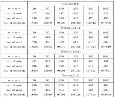
procedure to derive an NPI-B sample of size m = 3. There are n+mm = 63 = 20
orderings of 3 future observations among the 3 data observations, which are shown in Table 2.1. For example, (1,0,2,0) means there is 1 future observation fromI1, 0
fromI2, 2 from I3 and 0 from I4. All orderings have equal probability 1/20 = 0.05.
We sampled 200 NPI-B samples to record the number of frequencies of each ordering and put the results of the simulation in Table 2.1. It is clear from this table that the probability of each ordering is close to 0.05 in most cases.
In Banks’ bootstrap we use the same method but do not add the new value to the data set. Table 2.2 shows the orderings and probability of each one using multinomial distribution, and the observed proportions of each ordering using simulation with 200 Banks’ bootstrap samples. For a standard bootstrap sample, the value is drawn just from the data values. This sample can be, for example, (2,4,6) or (2,2,6) or (4,2,4) etc. There are 10 orderings that can appear here, as shown in Table 2.3. This table contains the probability of the ordering using a multinomial distribution with
ndata observations, and the actual probabilities of 200 standard bootstrap samples.
The theoretical probabilities and those from the simulation study are similar in most cases of the three kinds of bootstrap methods. Figure 2.1 illustrates the variance
standard-B
Orderings Theoretical Probabilities Frequency Observed Proportions
(3,0,0) 0.04 10 0.05 (2,1,0) 0.11 19 0.10 (2,0,1) 0.11 17 0.09 (1,2,0) 0.11 24 0.12 (1,1,1) 0.22 45 0.23 (1,0,2) 0.11 30 0.15 (0,3,0) 0.04 2 0.01 (0,2,1) 0.11 27 0.14 (0,1,2) 0.11 20 0.10 (0,0,3) 0.04 6 0.03
Table 2.3: Orderings of Standard-B
values of NPI-B samples, standard-B samples and Banks’ bootstrap samples to measure how far observations are spread out, and to give a general insight into the NPI-B samples that have a large variance. That is due to the method of sampling as discussed earlier. These values of variances come from the simulation experiment in this example and are plotted in Figure 2.1. There are some NPI-B samples which have small values of variance,and some of them are close to 0, as shown in Figure 2.1. This is possible with NPI-B samples but happens rarely. This can appear because the sample size is small.
2.3
NPI Bootstrap for Finite Intervals
The proposed nonparametric predictive inference bootstrap method (NPI-B) is based
on the repeated application of assumptionA(n). First it is done with then observed
data which createn+1 intervals, leading to one further observation. This is followed
by adding a further observation to the data and applying A(n+1) in order to draw
the second further observation, and so on. This is continued until there are m
fur-ther observations, which then togefur-ther (and without the original n observed data)
form one NPI-B sample. In this section we restrict attention to NPI-B applied to observations on a finite interval, because it simplifies the approach in the intervals
I1 and In+1. If NPI-B is applied on the full real-line, these two intervals require
different procedures for sampling a value within them. This will be presented in the following sections. The NPI-B algorithm for one-dimensional real-valued data on a finite interval is shown in Section 2.2.
2.3. NPI Bootstrap for Finite Intervals 29 ● ● ● ● ● ●
NPI standard Banks
0
5
10
15
The crucial difference from the standard bootstrap (’standard-B’) is that an NPI-B sample does not consist of the observations from the original sample but of points from the whole possible data range, because the sampling here is from the interval in between the data values and also outside the data range. This procedure leads to greater variation in the NPI-B samples than in the standard-B samples, as discussed in Section 2.2. Furthermore with NPI-B it is possible to estimateP(Y > c) for
dif-ferent values of c, especially if c is greater than the maximum value of the original
sample. This provides a method for estimating this probability, but the uniformity assumption within the intervals will affect the estimate and hence it would be dif-ficult to arrive at the exact statistical properties for such an estimate, hence the results presented mainly serve as an illustration of our method. It should be men-tioned that the NPI-B procedure is close in nature to Banks’ proposal of a smoothed bootstrap [8], where sampling also takes place uniformly in intervals between the
actual data, but Banks’ only uses the actual n+ 1 intervals from step 1 above for
the sampling of all values in the bootstrap sample, so a sampled value is not added to the data. This leads to a smaller variation in Banks’ approach than in NPI-B.
To study the NPI bootstrap performance, we have carried out a simulation exper-iment using R code. The considered methods in this part are: standard bootstrap, Banks’ bootstrap (smoothed Efron’s bootstrap) and NPI bootstrap. We have per-formed simulation studies, using the software R, for the performance of the NPI-B
as the estimation approach. For each method, we generated B = 1000 bootstrap
samples and calculated the variance which is the square of equation (1.6), bias from equation (1.9), absolute error |Tn∗−To
n|. Tno here is the observed value of
statis-tic which is calculated from the original sample. We found the absolute error for every value of statistics in bootstrap samples and then took the average of these values, and the mean square error (MSE) of the statistics from equation (1.12). It is important to mention the reason for choosing these measures. The variance of statistics is used to show the difference between the three methods of bootstrap or to show which method has a close variance to the original observations. We will see that the NPI-B has the largest variance of statistics but it is the closest one to the
2.3. NPI Bootstrap for Finite Intervals 31
n Uniform (0,1) Beta (1,2) Beta (0.5,1) 20 0.0800 0.0551 0.0729 50 0.0815 0.0444 0.0738 100 0.0857 0.0523 0.0799 200 0.0853 0.0492 0.0825 500 0.0842 0.0523 0.0859 1000 0.0841 0.0521 0.0834
Table 2.4: Variances of original samples from specific distributions with a variety of sample sizes
method measures n= 20 n= 50 n= 100 n= 200 n= 500 n= 1000 standard variance of mean 0.004 0.002 0.001 0.0005 0.0002 0.0001
bias 0.003 -0.0001 -0.001 -0.001 0.0002 0.0001 absolute error 0.049 0.032 0.024 0.017 0.010 0.007
MSE 0.004 0.002 0.001 0.0005 0.0001 0.0001 Banks variance of mean 0.004 0.002 0.001 0.0004 0.0001 0.001
bias -0.007 0.001 0.0003 0.001 -0.0001 -0.0001 absolute error 0.052 0.032 0.023 0.017 0.010 0.007
MSE 0.004 0.002 0.001 0.0004 0.0002 0.0001 NPI variance of mean 0.008 0.003 0.002 0.001 0.0003 0.0002 bias -0.009 0.002 0.001 0.001 -0.0002 0.00001 absolute error 0.070 0.046 0.033 0.024 0.015 0.010
MSE 0.008 0.003 0.002 0.001 0.0003 0.0002
Table 2.5: The sample mean when the original sample was from U (0,1)
variance of the original sample. Regarding bias, MSE and absolute error, they are the most commonly used measures of statistical accuracy of estimators as discussed in Section 1.3.1. We repeated this experiment forn= 20,50,100,200,500,1000 and for statistics: mean, variance and upper quartile (q75), to present location, variation
and position parameters, respectively, and for different distributions such as Uni-form (0,1), Beta (α, β), with (α = 0.5, β = 1) and (α = 1, β = 2), as examples of symmetric and skewed distributions. Note that, in these cases, the size of bootstrap
samples ism = n. Table 2.4 shows the observed variance of these original samples
with various sample sizes.
Tables 2.5, 2.6, 2.7, of Uniform (0,1) show that when comparing the absolute value of bias, the NPI bootstrap has the smallest bias of variance parameter in all cases, but for the mean andq75it has the smallest value only ifnis very large (500 or
1000). Mostly, for three parameters, the MSE and absolute error of Banks’ bootstrap and standard bootstrap are very close but they are less than NPI bootstrap’s values of MSE and absolute error. The variance of three parameters using NPI-B is larger than the others methods. This property of NPI-B is considered a good point because