Macroeconomic Factors and Micro-Level Bank Risk

Macroeconomic Factors and

Micro-Level Bank Risk

Claudia M. Buch

Sandra Eickmeier

Esteban Prieto

CES

IFO

W

ORKING

P

APER

N

O

.

3194

C

7:

M

P

I

F

S

2010

PRESENTED AT CESIFO AREA CONFERENCE ON MACRO, MONEY & INTERNATIONAL FINANCE, FEBRUARY 2010

An electronic version of the paper may be downloaded

• from the SSRN website: www.SSRN.com

• from the RePEc website: www.RePEc.org

CESifo Working Paper No. 3194

Macroeconomic Factors and

Micro-Level Bank Risk

Abstract

The interplay between banks and the macroeconomy is of key importance for financial and economic stability. We analyze this link using a factor-augmented vector autoregressive model (FAVAR) which extends a standard VAR for the U.S. macroeconomy. The model includes GDP growth, inflation, the Federal Funds rate, house price inflation, and a set of factors summarizing conditions in the banking sector. We use data of more than 1,500 commercial banks from the U.S. call reports to address the following questions. How are macroeconomic shocks transmitted to bank risk and other banking variables? What are the sources of bank heterogeneity, and what explains differences in individual banks’ responses to macroeconomic shocks? Our paper has two main findings: (i) Average bank risk declines, and average bank lending increases following expansionary shocks. (ii) The heterogeneity of banks is characterized by idiosyncratic shocks and the asymmetric transmission of common shocks. Risk of about 1/3 of all banks rises in response to a monetary loosening. The lending response of small, illiquid, and domestic banks is relatively large, and risk of banks with a low degree of capitalization and a high exposure to real estate loans decreases relatively strongly after expansionary monetary policy shocks. Also, lending of larger banks increases less while risk of riskier and domestic banks reacts more in response to house price shocks. JEL-Code: E44, G21.

Keywords: FAVAR, bank risk, macro-finance linkages, monetary policy, microeconomic adjustment.

Claudia M. Buch

University of Tübingen / Germany claudia.buch@uni-tuebingen.de

Sandra Eickmeier

Deutsche Bundesbank / Germany sandra.eickmeier@bundesbank.de

Esteban Prieto

University of Tübingen / Germany esteban.prieto@wiwi.uni-tuebingen.de

27 September 2010

The views expressed in this paper do not necessarily reflect the views of the Deutsche Bundesbank. The paper has partly been written during visits of C.M. Buch and E. Prieto to the research centre of the Deutsche Bundesbank. The hospitality of Bundesbank is gratefully acknowledged. We would like to thank Falko Fecht, Heinz Herrmann, Thomas Laubach as well as the participants of the Annual Meeting of the Monetary Group of the Verein für Socialpolitik, held in Gerzensee in February 2010, at

the CESifo Conference on Macro, Money, and International Finance (Munich, Februar 2010), at a seminar at the Bundesbank, at the 16th International Conference on Computing in Economics and Finance (London, July 2010) and the Annual Conference of the Verein für Socialpolitik (Kiel,

September 2010) for most helpful comments on an earlier version of this paper. All errors and inconsistencies are solely in our own responsibility.

1 Motivation

How are macroeconomic shocks transmitted to bank risk and other banking variables? What are the sources of bank heterogeneity, and what explains differences in individual banks’ responses to macroeconomic shocks? We provide answers to these questions by analyzing the exposure of banks to macroeconomic developments in the U.S. over the period 1985-2008. Our analysis is based on a factor-augmented vector autoregressive model (FAVAR) in the tradition of Bernanke et al. (2005) which extends a standard macroeconomic VAR comprising GDP growth, inflation, house price inflation, and the monetary policy interest rate with a set of factors summarizing a large amount of information from bank-level data. Our bank-level dataset contains bank risk which is our focus. We also include bank capitalization, profitability, and loans as bank-level variables which affect the transmission mechanism of macroeconomics shocks on risk. Data for a balanced panel of about 1,500 banks are taken from the U.S. call reports. We decompose the banking data into common and idiosyncratic components. A set of macroeconomic (supply, demand, monetary policy and house price) shocks is identified and, based on an impulse response analysis, their transmission through the banking system is assessed. We look at the effects of the shocks not only on aggregate bank variables, but we also on individual banks. Using cross-sectional regressions, we study which bank-level features can explain differences in banks’ responses to macroeconomic shocks.

Our main findings are as follows. (i) Average bank lending increases following expansionary shocks. Average bank risk declines after most expansionary macroeconomic shocks. House price and monetary policy shocks are particularly important for bank risk. (ii) There is a substantial degree of heterogeneity across banks both in terms of idiosyncratic shocks and the asymmetric transmission of common (banking and macroeconomic) shocks. While average risk declines, risk of a sizeable fraction of banks rises in response to expansionary shocks. The degree of capitalization, the exposure to real estate loans, the riskiness and the presence of foreign affiliates matter for individual banks’ risk responses.

Our study is related to theoretical and empirical work on the effects of macroeconomic (mostly monetary policy) developments on bank risk. Financial accelerator mechanisms imply that changes in interest rates may have countervailing effects on bank risk. On the one hand, lower interest rates reduce the interest rate burden for firms, lower the risk of outstanding flexible loan contracts, thereby increasing the probability of repayment and the value of the underlying collateral. On the other hand, the borrowing capacity of high-risk firms increases with the value of pledgeable assets. Also, banks might engage in riskier, high yield, projects to offset the negative effects of lower interest rates on profits. Risk might increase. Conversely, higher interest rates increase the agency costs of lending, banks reduce

the amount of credit to monitoring-intensive firms, and they invest more in safe assets (“flight-to-quality”) (Bernanke et al. 1996, Dell’Ariccia and Marquez 2006, Matsuyama 2007).

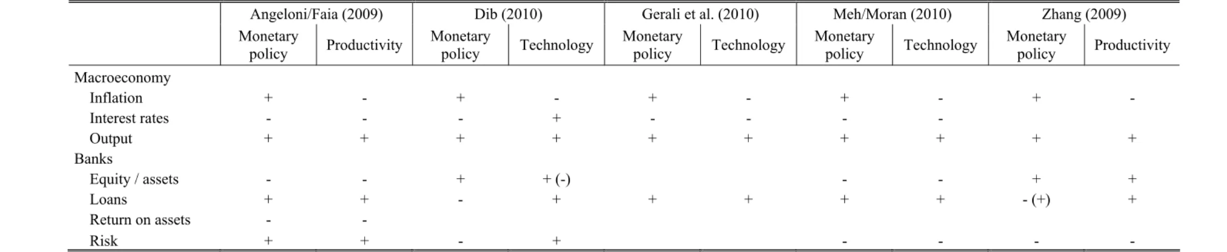
While the original financial accelerator models do not assign a specific role to banks, recent macroeconomic models explicitly analyze the feedback between banks and the macroeconomy in the context of dynamic stochastic general equilibrium (DSGE) models (Angeloni and Faia 2009, Dib 2010, Gerali et al. 2010, Meh and Moran 2010, Zhang 2009).1 In these models, the impact of expansionary shocks on bank lending is unequivocally positive, but the impact on bank risk is less clear cut (Appendix 1 and Table A.1). In Angeloni and Faia (2009), for instance, a declining interest rate, following a positive supply or monetary policy shock, reduces banks’ funding costs and increases the probability to repay depositors. To maximize profits, banks optimally choose to increase leverage. But the decline in interest rates also lowers banks’ return on assets and this, together with higher leverage, increases bank risk. In Zhang (2009), on the contrary, expectations of future outcomes play a central role. A positive technology shock, for instance, increases the return on capital above its expected value which in turn corresponds to a lower than expected loan default rate. The bank thus realizes unexpected profits on its loan portfolio. Bank capital is accumulated through these earnings, strengthening banks’ balance sheet positions and reducing risk. A small set of empirical papers looks at the impact of monetary policy shocks on bank risk, with ambiguous findings. A few recent papers analyze the risk-taking channel of monetary policy and investigate whether low policy interest rates encourage lending to high-risk borrowers (Rajan 2005, Borio and Zhu 2008). Empirical studies based on bank-level data find evidence that lower interest rates increase bank risk (Altunbas et al. 2009, Gambacorta 2009, Ioannidou et al. 2009, Jiménez et al. 2007).2 Based on time series evidence for the U.S., Eickmeier and Hofmann (2010) and Angeloni et al. (2010) find a decline of various credit risk spreads and an increase of bank balance sheet risk, respectively, following a positive monetary policy shock. Using a model that captures the feedback between bank-level distress and the macroeconomy, De Graeve et al. (2008), in contrast, find a decline in German banks’

1 _{These models differ with regard to the financial frictions (demand- versus supply-side), the assumptions on the} degree of competition in the banking sector, the modeling of bank risk, the stickiness of interest rates, and the types of macroeconomic shocks.

2

The risk-taking channel focuses on the incentives to engage in ex ante riskier projects. We instead measure

changes in bank risk ex post. Our data do not allow isolating changes in the structure of the existing portfolios of

banks and the structure of new lending (Jiménez et al. 2007). Also, we do not control for the duration of a particular monetary policy stance but consider “average” shocks over the entire sample period (Altunbas et al. 2009). For these reasons, our results are not directly comparable with results for the risk-taking channel of monetary policy.

probability of distress after a monetary policy loosening. The impact of other shocks has, to the best of our knowledge, so far not been subject to careful empirical investigation.3

Our modeling approach implicitly accounts for the key mechanisms stressed in the theoretical papers and provides empirical evidence on the net effect of macroeconomic shocks on bank

risk.

Our main research question, the exposure of banks to macroeconomic factors, also features prominently in recent proposals for regulatory reforms (Basel Committee 2009). Rochet (2008) suggests on the basis of a theoretical model that banks should face a capital requirement and a deposit insurance premium that increases with their exposure to macroeconomic factors. Farhi and Tirole (2009) analyze the incentives of banks to coordinate their exposure to macroeconomic shocks, and they argue that banks which react more to macroeconomic factors should be regulated more tightly. Gersbach and Hahn (2009) propose a regulatory framework under which a banks’ required level of equity capital depends on the equity capital of its peers and, in this sense, on the macroeconomic environment. Implementing these proposals requires information about individual banks’ exposures to macroeconomic factors. Our results inform this debate.

We make several contributions. First, the FAVAR model allows analyzing the dynamic interaction between bank-specific and macroeconomic developments in a flexible way. Several VAR-studies allow for the interaction between credit and macroeconomic factors (e.g. Ciccarelli et al. 2009, Eickmeier et al. 2009), but these studies do not focus on bank risk or bank-specific effects. Bank-level studies on the risk-taking or bank lending channel, in contrast, allow macroeconomic factors to affect bank risk, but macroeconomic factors are not modeled as a function of banking variables. Our setup accounts for the endogeneity of both, macroeconomic- and banking factors.

Second, the FAVAR allows including lots of bank-level data. The factor model exploits the comovement between individual banks and allows us to model linkages between individual banks, i.e. through the interbank market or the exposure to common shocks. The need to account for linkages between financial institutions is one key lesson of the recent crisis (Brunnermeier 2008, IMF 2009). Moreover, we model the interaction between different banking variables, including the risk and the return of banks, and thus accounting for the fact that, in “search for yield”, banks may increase risk (Hellwig 2008, Rajan 2005). Another important implication of the fact that we can include lots of bank-level data in our model is that we can assess the exposure of each individual bank to macroeconomic shocks.

3

Altunbas et al. (2009) find that higher GDP growth lowers bank risk but changes in asset prices have no clear-cut impact in risk. The analysis of these factors in risk is, however, not the focus of their paper. Moreover, the authors do not identify structural (real or asset price) shocks.

Third, previous papers analyzing the bank lending channel or the risk-taking channel regress bank-level lending or risk on the monetary policy interest rate, GDP growth, or asset prices (e.g. Altunbas et al. 2009, Cetorelli and Goldberg 2008, Ioannidou et al. 2009, Jiménez et al. 2007, Kashyap and Stein 2000).4 The macroeconomic indicators are reduced-form constructs, and their developments may reflect the pass-through of different types of shocks. Instead, we consider identified orthogonal macroeconomic shocks which allow us to better disentangle the common drivers of banking developments.

Fourth, FAVAR models have previously been fitted to large macroeconomic datasets (e.g. Bernanke et al. 2005, Boivin and Giannoni 2008) or aggregate financial datasets (e.g. De Nicoló and Lucchetta 2010, Eickmeier and Hofmann 2010). The methodology, however, allows exploiting even richer information, and its application also to micro-level data is the natural next step. We will show that omitting bank-level information might bias estimates of impulse responses and shocks series. Our study is one of the first using a FAVAR model linked to a micro-level dataset. It is closely related to Dave et al. (2009) who use a similar modeling approach for U.S. data but focus on the bank lending channel while our focus is on risk.5

In Sections 2 and 3, we present the data and the FAVAR methodology, respectively. In Section 4, we provide and discuss the empirical results and conclude in Section 5.

2 The

Data

The key feature of our empirical model is the joint analysis of macroeconomic data and bank-level data, which we describe in this section. We also compare our risk measure to alternative risk measures used in the literature and address potential concerns regarding the presence of a factor structure in the data.

2.1

Macroeconomic Data

Our set of macroeconomic variables comprises log differences of real GDP, the GDP deflator, real house prices, and the level of the effective Federal Funds rate. Real house prices are measured as the Freddie Mac Conventional Mortgage house price, divided by the GDP deflator. The data are retrieved from FreeLunch.com, a free internet service provided by Moody’s Economy.com.

4 _{These papers on risk-taking address the issue that monetary policy is endogenous by either approximating} monetary policy of the countries studied by foreign policy rates (Jiménez et al. 2007) or by Taylor rule gaps, i.e. deviations of the policy rate from the rate implied by the Taylor rule (Altunbas et al. 2009).

5

Other papers combining factor models and micro-level data (with a different focus) are Den Reijer (2007) and Otrok and Pourpourides (2008).

2.2

Bank-Level Data

Our source for bank-level data is the Consolidated Report of Condition and Income (call reports) that all insured commercial banks in the United States submit to the Federal Reserve each quarter. A complete description of all variables is provided in Appendix 3. From the call reports, we compile a dataset consisting of quarterly income statements and balance sheet data over the period 1985Q1–2008Q2, i.e. our analysis does not include the period following the bankruptcy of Lehman Brothers. (See Frankel and Saravelos (2010) for a similar definition of the pre-crisis period.) Using instead information up to the beginning of the Great Recession in the fourth quarter of 2007 does not qualitatively change our main results.

We consider the following banking variables. Bank risk is measured using the share of non-performing loans in total loans. The (unweighted) ratio of equity capital to total assets is used as a measure of bank balance sheet strength. Our measure of banks’ profitability is return on assets, defined as net income to total assets. Finally, we include (growth of) total bank loans. 2.2.1 Balancing the Panel, Correcting for Outliers, and Preparing the Data for the Factor

Analysis

Following previous micro banking studies, we apply a number of screens to exclude implausible and unreliable observations. We exclude observations with (i) negative or missing values for total assets, (ii) negative total loans, (iii) loan-to-assets ratios larger than one, or (iv) capital-to-assets ratios larger than one. In addition, entire banks with gross total assets below $25 million and banks engaged in a merger are dropped from the sample.6

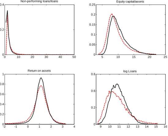
Finally, if one of the three ratios (non-performing loans-to-total loans, capital-to-assets, and net income-to-assets) of an individual bank falls in the bottom or top percentile at any point in time, the entire bank is dropped. We only include banks which are in business during the entire period under study. Overall, these corrections reduce the sample from 13,375 banks in the unbalanced panel to 1,512 banks in the balanced panel. Figure 1 shows that balancing has not much changed the distribution of the data.

The bank-level data are treated in the usual manner for factor analysis. All series are seasonally adjusted, and they enter the dataset as stationary variables. Because loans are assumed to be integrated of order 1, we include them as log differences in our model. The balance sheet ratios can be considered stationary, hence there is no need to difference them. The stationary series are then demeaned, and structural breaks in the means are accounted for.7 _{Moreover, the series are standardized to have unit variance, and outliers are removed.}

6 _{Berger and Bouwmann (2009) state that banks with total assets below $25 millions are not likely to be viable} commercial banks.

7

Some ratios do not seem to revert to a constant mean. This is possibly due to regulatory changes which led to an adjustment in capital ratios and other banking variables. To account for these changes, we detect breakpoints by applying the sequential multiple breakpoint test of Bai and Perron (1998, 2003) (and the Gauss routines

Outliers are defined as observations with absolute median deviations larger than six times the interquartile range. They are replaced by the median value of the preceding five observations (Stock and Watson 2005).

2.2.2 Measuring Bank Risk

The non-performing loans ratio is our main measure of bank risk. It captures the asset risk of banks and thus the share of bank loans that are actually in default. This measure is available for a large number of banks for a long time period. Another advantage is that it is not much affected by changes in accounting standards. Also, it matches up with theoretical models that describe banks as intermediaries between depositor and lenders and that consider loan defaults as the main source of instabilities in banking (e.g. Boyd and De Nicoló 2005, Martínez-Miera and Repullo 2010, Zhang 2009).

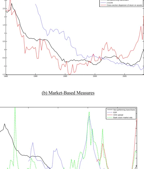
Alternative measures of bank risk have been used in the literature as well (see, e.g. Beck 2008 for a survey), and Figure 2 shows how they are related to the non-performing loans ratio. The

z-score measure is calculated using information on banks’ level of equity, the standard

deviation of profits, and profits. Loosely speaking, the z-score is inversely related to the

probability that the bank’s equity base is eroded, e.g. higher values indicate less risk. Although the focus of this risk measure differs from the non-performing loans ratio, the z

-score for the U.S. banking system tracks the median non-performing loans ratio quite well (Figure 2a). The disadvantage of the z-score is that it requires calculating the volatility of

profits over a certain time window, the choice of which is somewhat arbitrary.8 _{Figure 2a also}

reveals that the non-performing loans ratio is highly correlated with the cross-section dispersion of individual banks’ return on assets. This measure is the banks’ counterpart of the cross-section dispersion of firms’ earnings which has been used in the literature to capture uncertainty or risk in the business sector (as, e.g., discussed in Bloom 2009).

Finally, we have checked how more market-based measures of bank risk are related with the median non-performing loans ratio (see Figure 2b). We have used CDS spreads obtained from Bloomberg, EDFs from Moody’s KMV, and stock market volatility (source: Goldman Sachs).9 _{One disadvantage of these measures is that they are not available for the full sample}

period or for all banks. CDS spreads and EDFs trace the non-performing loans ratio reasonably well. These market-based measures, however, tend to peak in times of financial market stress. The non-performing loans ratio, in contrast, shows a much smoother pattern and arguably tracks fundamental risk of banks in a more reliable way.

provided by Pierre Perron on his webpage) to all series of our (stationary) dataset, and we subtract the (possibly shifted) means from the series (see Eickmeier 2009 for a similar treatment of (macroeconomic) data in a factor modelling setup). When we, instead, linearly detrend the series, the results are basically unaffected.

8

Related to this, the z-score, as it is shown in Figure 2, by construction, lags the non-performing loans ratio.

2.2.3 Is There a Factor Structure in the Data?

Exploiting a rich amount of (bank-level) information can be beneficial in a factor analysis. Our factor model, however, also needs to provide a good description of the data. For this to be the case, there needs to be a factor structure among the series included, or, put differently, factors can be accurately estimated only if the series strongly co-move (Boivin and Ng 2006). This issue is particularly relevant for microeconomic data as opposed to (aggregate) macroeconomic data to which factor models have been previously employed and which tend to exhibit a greater comovement.

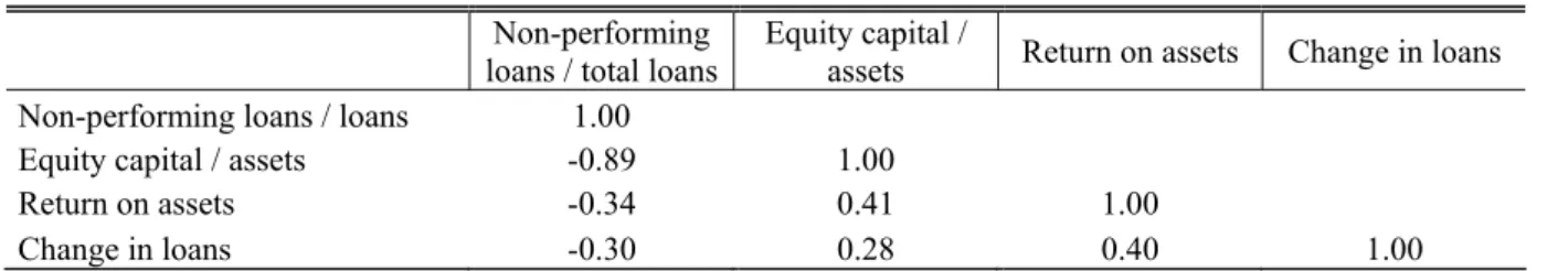
We first assess to what extent the different banking variables (risk, capitalization, return, lending) are correlated. Table 1 shows that the medians are highly correlated. The non-performing loans ratio and capitalization are particularly strongly (negatively) correlated because a decline in asset quality forces banks to write down assets. The correlation is, however, not perfect. Unlike the non-performing loans ratio, capitalization is also determined by regulatory requirements. Moreover, banks use it as a signaling devise and might avoid adjustments in response to negative macroeconomic shocks.

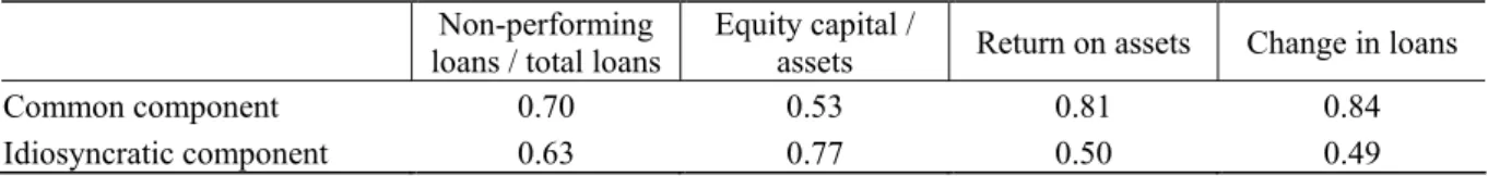
We next examine to what extent individual banks are related. Table 2 shows the variance shares explained by the first 15 principal components extracted separately from bank-level datasets associated with each of the four variables. There is reasonably strong comovement among banks for all banking variables with 6 factors explaining at least 40 percent and 9 factors explaining at least 50 percent of the variation in the ratios. The comovement is a bit lower for loan growth where 7 and 12 factors are needed to explain 40 and 50 percent, respectively.

We have carried out further robustness checks. We have first removed cross-sectional outliers from the dataset, i.e. we have dropped banks from the sample with absolute median deviations larger than six times the interquartile range (on average over the sample period).10

We have also downweighted each bank-level series by the inverse of the standard deviation of its idiosyncratic component (weighted principal components, see Boivin and Ng 2006). Finally, we have aggregated the balance sheets of all banks that belong to the same bank holding company. This alternative dataset contains 560 bank holding companies, and we have extracted factors from this dataset. Bank holding companies may be able to shift resources among the banks they control (Kashap and Stein 2000), and we would expect the comovement between bank holding companies to be larger than between individual banks. The factors extracted from our original dataset and the factors estimated in these robustness checks are very highly correlated. The trace R² from a regression of the principal components

extracted from the original dataset on the principal components estimated from the modified datasets lie between 0.95 and 0.99.11

As a final check, we have assessed whether omission of regional banking factors affect our estimation of the national factors. We have separately extracted factors from the bank-level data by state using principal components. We have then pooled the state-level factors and estimated national factors from the pooled dataset (see, e.g., Del Negro and Otrok 2007, Kose et al. 2003, Mönch et al. 2009, Beck et al. 2009 for alternative approaches).12 The trace R²

from a regression of the principal components extracted from the entire dataset on the principal components extracted from the set of state-level factors is, again, very high (0.99). Hence, neglecting regional factors does not seem to affect our nation-wide factor estimation.

3 The FAVAR Methodology

With the bank-level variables at hand, we next describe how we use this information to model the dynamic feedback effects between U.S. banks and the macroeconomy. We start from a small-scale macroeconomic VAR model which includes GDP growth (Δyt), GDP deflator

inflation (Δpt), the Federal Funds rate ( ffrt), and real house price inflation Δhptas

endogenous variables. These variable are summarized in an M( 4) 1= × -dimensional vector

[

]

t t t t t

G = Δ Δ Δy p hp ffr . GDP growth, inflation, and interest rates represent the standard

block of variables included in macroeconomic VARs (e.g. Christiano et al. 1996, Peersman 2005); fewer studies also include house prices in such a VAR (Bjørnland and Jacobsen 2008, Jarociński and Smets 2008). We include house prices not only because they may be relevant for the macroeconomy but also because they reflect the value of assets that can potentially serve as collateral for bank lending.

We augment the vector G_t with a set of r “banking factors” B_t which yields the r+M×1

-dimensional vector F_t =

[

]

[

]

We model the joint dynamics of macroeconomic variables and banking factors as a VAR(p)

process:

A( )FL _t = +c Pw_t, (1)

11

The comparison is based on the first 6 principal components because 6 latent factors are also used in our analysis below. Below, we will explain this choice of the number of factors.

12 _{More precisely, of the 50 states in the U.S. we consider only the states with at least 10 banks (which would} result in at least 40 series per state). This leaves us with 40 states. We estimate the state-level factors as the first 6 principal components from bank-level data for each of the 40 states. We pool the estimated state-level factors, extract the first 6 principal components from the 240 (= 6μ40) state-level factors, and compare them with the first 6 principal components estimated from the entire dataset.

where A( ) A₁ ... A p p

L = −I L− − L is a lag polynomial of finite order p, c comprises

deterministic terms,13 and w_t is a vector of structural shocks which can be recovered by imposing restrictions on P .

Let the elements of F_t be the common factors driving the N×1 vector X_t which summarize our four banking variables (loan growth, the non-performing loans ratio, return on assets, and the capital ratio) of 1,512 individual banks. To assess the impact of macroeconomic shocks on the “average” bank, we also include in X_t the medians of the four banking variables.14 Hence, the cross-section dimension is N = 6,052 (= 1,512×4 + 4).

It is assumed that X_t follows an approximate dynamic factor model (Bai and Ng 2002, Stock and Watson 2002):

X_t = Λ'F_t + Ξ_{t, (2)}

where Ξt =

[

]

15 _{The matrix}

of factor loadings Λ =

[

]

1

r+M× , and r+M <<N holds. Common and idiosyncratic components are orthogonal,

the common factors are mutually orthogonal, and idiosyncratic components can be weakly mutually and serially correlated in the sense of Chamberlain and Rothschild (1983). Equations (1) and (2) represent a FAVAR model as has been introduced by Bernanke et al. (2005).16

The model is estimated in five steps.

First, the dimension of F_t, i.e. the overall number of common factors r+M , is determined to

be 10. These include the 4 observable macroeconomic factors and the r=6 latent banking factors. We make this choice because our main results change when the number of factors is lowered, but are barely affected when it is increased, and because we prefer a sparse parameterization.

In the second step, we estimate B_t by removing the observed factors from the overall factor space. We do this with the aid of the iterative procedure proposed by Boivin and Giannoni (2007). We obtain an initial estimate of B_t, ˆB(0)

t , as the first r =6 principal components of

X_t. Then we regress X_t on ˆB(0)

t and Gt, ending up with ) 0 (

ˆ

G

Λ , the coefficients (or factor

13 _{As the observables are not demeaned, we include constants.}

14 _{To save time and capacity, we will compute confidence bands only for these median variables but we will} focus on point estimates for individual banks’ responses. Point estimates of median impulse response functions are very similar to point estimates of impulse response functions of the median bank.

15 _{Note that}

Ft can contain dynamic factors and lags of dynamic factors. Insofar, equation (2) is not restrictive.

16 _{Bernanke et al. (2005) are interested in a monetary policy shock and include the Federal Funds rate as the} only observable in the FAVAR. Our model most closely resembles the one used in Eickmeier and Hofmann (2010) which models a set of latent factors estimated from lots of non-financial sector balance sheet items and other financial variables.

loadings) that belong to G_t. We calculate _X(0) _{=X − Λ}ˆ(0)_G

t t G t and estimate

(1)

ˆBt as the first r

principal components of _X(0)

t . This procedure is repeated until convergence,

17 _{and we end up}

with the estimator of B_t, ˆBt.

The latent banking factors together with the observable macroeconomic factors explain 43 percent of the variation in the bank-level dataset which represents a reasonable degree of comovement between the banking variables.

Third, a VAR(1) model is fitted to ⎡_⎣G ' B ' '_t ˆ_t ⎤_⎦ . The lag order of 1 is suggested by the BIC. Fourth, we identify macroeconomic shocks combining sign restrictions and zero contemporaneous restrictions, as will be explained shortly.

In the fifth and final step, confidence bands of the impulse response functions are constructed using the bootstrap-after-bootstrap technique proposed by Kilian (1998). This technique allows removing a possible bias in the VAR coefficients which can arise due to the small sample size. The number of bootstrap replications equals 500. Notice that, since N >T, we

neglect the uncertainty involved with the factor estimation, as suggested by Bernanke et al. (2005).

As regards the fourth step, the identification of macroeconomic shocks, we apply sign restrictions on short-run impulse response functions (e.g. Canova and De Nicoló 2003, Faust 1998, Peersman 2005, Uhlig 2005) and contemporaneous zero restrictions. The identification scheme is implemented in two steps. The first step involves carrying out a Cholesky decomposition of the covariance matrix of the reduced form VAR residuals. We impose the following ordering: Δ → Δ → Δyt pt hpt → ˆBt → ffrt. We label the Cholesky residuals

associated with the equations explaining house price inflation, the r latent banking factors’

and the Federal Funds rate “house price shock”, “shocks to the banking factors” (or “banking shocks”) and “monetary policy shocks”, respectively. We should note that we cannot be sure that the shocks to the banking factors truly represent shocks that occur in the banking sector or “banking shocks”. They may instead also contain shocks that are not modeled explicitly, such as shocks to balance sheets of the non-financial private sector (which may, however, also be propagated through the banking system).

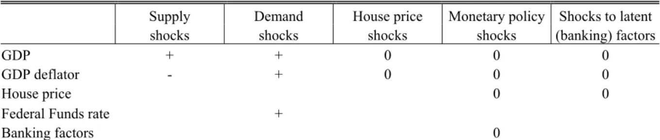
The second step aims at disentangling “aggregate supply shocks” and “aggregate demand shocks”. It involves rotating the Cholesky residuals associated with the equations for GDP growth and GDP deflator inflation and imposing the following theoretically motivated sign restrictions. After an aggregate supply shock, GDP and the GDP deflator move in opposite directions whereas after an aggregate demand shock, these two variables as well as the

17

We define the procedure as having converged if the sum of squared residual from a regression of x ,_it i=1,...,N on

( ) ˆBj

t and Gt has hardly changed compared to the sum of squared residual from a regression of x ,it i=1,...,N on

( 1) ˆB j−

t

Federal Funds rate move in the same direction. The sign restrictions are imposed contemporaneously and on the first four lags after the shock. Results are robust with respect to the restricted number of lags. The identifying restrictions are summarized in Table 3, and in Appendix 2 we explain how we identified the shocks in more detail.

The sign restrictions are consistent with standard theoretical models.18 The ordering implies that GDP as well as aggregate and house prices do not react contemporaneously to banking and monetary shocks, which is fairly standard in SVAR studies. GDP and the overall price level react with a delay to house price movements (e.g. Jarociński and Smets 2008). Moreover, we allow the monetary policy instrument to respond contemporaneously to all shocks. By ordering the policy instrument below the banking factors, we follow most of the SVAR literature which models macroeconomic and banking variables together (Ciccarelli et al. 2009). Reasons for sluggish adjustment of the banking sector to monetary policy could be the need to renegotiate existing contracts or close customer relationships that banks do not want to interrupt. Consistent with this assumption, the empirical banking literature finds that interest rate spells of banks are sticky and do not react quickly to market interest rates (Berger and Hannan 1991).

4 Empirical

Results

We organize the presentation of our empirical results around our two main research questions.

4.1

How are Macroeconomic Shocks Transmitted to the Banking Sector?

4.1.1 Impulse Response Functions of Bank Risk and Other Banking Variables

To look at how macroeconomic shocks are transmitted to macroeconomic variables we present in Figure 3 impulse response functions of GDP, the GDP deflator, house prices, and the Federal Funds rate to aggregate supply, aggregate demand, monetary policy, and house price shocks. We show median responses together with 68% confidence bands to shocks of the size of one standard deviation.

After a supply shock, GDP rises and the GDP deflator falls permanently. The demand shock triggers a temporary increase in GDP, and the general price level rises permanently. The monetary policy rate does not change significantly after the supply shock, but it rises temporarily after the demand shock. An expansionary monetary policy shock leads to a temporary rise in economic activity (consistent with long-run real neutrality of monetary policy) and to a permanent rise in the GDP deflator. We do not observe a price puzzle, i.e. a decline of the price level after an expansionary monetary policy shock. This is reassuring

since it suggests that we have accurately identified monetary policy shocks. House price shocks trigger responses which are reminiscent of demand shocks: Economic activity, the general price level, and the monetary policy rate rise. The increase in GDP after the house price shock is, however, barely significant. House prices themselves react sluggishly to macroeconomic shocks. Their reaction roughly mirrors the reaction of the GDP deflator. Overall, the response of the macroeconomic variables is in line with previous evidence.

To assess the dynamic transmission of macroeconomic shocks to the banking sector, we look at impulse response functions for the median bank (Figure 4). While theory provides consistent predictions concerning the response of bank loans and returns following expansionary shocks, predictions concerning the adjustment of bank risk and capital are less clear cut. Loans indeed increase after all expansionary shocks. It takes roughly a year before loans increase after monetary policy shocks (whereas they rise immediately after the other shocks). This pattern for monetary policy shocks has already been found in other studies (e.g. Christiano et al. 1996). Banks’ returns are positively correlated with the responses of the Federal Funds rate to macroeconomic shocks, although the magnitude and timing of the effects differ depending on the shock.

Risk declines following monetary policy, demand, and house price shocks. The effects last between two quarters (after the demand shock) and about four years (after the monetary policy shock). These results are in line with the prediction in Zhang (2009) that an expansionary monetary policy shock increases credit supply by reducing funding cost. Ex post loan default rates go down which feeds back into better capitalization. The evolution of the capital-asset ratio mirror-images the evolution of the non-performing loan ratio in qualitative terms after the supply and the monetary policy shocks but not after the demand and the house price shocks.

Bank risk increases in response to supply shocks. Following a positive supply shock, the balance sheet composition tilts towards higher leverage (a lower capital-to-asset ratio) and higher risk, consistent with Angeloni and Faia (2009). In their model banks’ default probability is determined by the distribution of the return on lending, the liquidation value of the projects and, indirectly, by the leverage ratio. However, a positive supply shock might also increase the dispersion of the return to lending if more high risk entrepreneurs enter the market. This increases risk in their model and would be in line with our finding.

Our result of a decline in bank risk after expansionary monetary policy shocks is therefore similar to the findings by De Graeve et al. (2008) (for Germany) but not to those from other empirical studies such as Angeloni et al. (2010) or from the risk-taking channel literature. The correlation between banks’ risk and return is negative after the demand and the house price shocks. This would be consistent with theoretical models arguing that banks with higher returns (and thus presumably higher market power) engage in less risky lending than banks

with lower returns (Allen and Gale 2004, Martínez-Miera and Repullo 2008). The correlation between bank returns and risk after the supply and the monetary policy shocks depends on the horizon; it is positive at short horizons but becomes negative at medium horizons. Recent DSGE models have different implications on the correlation between risk and return. Following a monetary policy shock, this correlation is negative in Angeloni and Faia (2010) but positive in Meh and Moran (2010) or Zhang (2009).

4.1.2 Variance Decompositions

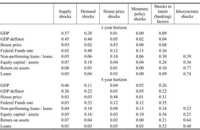
While Figure 4 provides information on the dynamic responses of (median) bank-level variables to macroeconomic shocks, Table 4 shows the forecast error variance decomposition and allows assessing the relative importance of each of these shocks. We distinguish the short run (the one-year forecast horizon) from the medium run (the five-year horizon). Macroeconomic shocks together explain 27 percent of the non-performing loans ratio, 33 percent of the capital ratio, and 12 and 14 percent of returns on assets and loans, respectively, of the median bank in the short run. These numbers increase for the ratio variables by 1-8 percentage points in the medium run and decline for loans by 2 percentage points. For risk at short horizons, house price shocks are most important, consistent with theoretical models that emphasize the role of real estate as collateral for bank loans (Goel et al. 2009). Monetary policy shocks play the biggest role for risk at medium horizons. Aggregate demand shocks account for the greatest share of the variation in loans at short horizons. At medium horizons, all shocks play an about equally discernible role for loans. An additional finding is that the idiosyncratic (variable-specific) components are about as important as common banking shocks for the non-performing loans and the capital ratios and they are more important for return on assets and loans.

Table 4 also reveals that shocks to the latent banking factors (or “banking shocks”) are quite important for macroeconomic variables. These shocks explain between 22 and 35 percent of the forecast error variance of the macroeconomic variables in the medium run. The shares are largest for house prices and for the monetary policy rate. The short-term effects are smaller, ranging between 4 percent (GDP deflator) and 26 percent (Federal Funds rate).

4.1.3 The Role of Bank-Level Information

We finally assess how omitting information extracted from the micro-level banking dataset would bias our results. Figure 5 compares the impulse responses of the observable macroeconomic factors derived from our benchmark FAVAR model with impulse responses obtained from a VAR in which we replace the banking factors by the median values of our bank-balance sheet variables. The responses of GDP, the GDP deflator, and house prices following macroeconomic shocks are very similar in magnitude and shape in both models. There are, however, notable differences in the responses of the Federal Funds rate after all

four shocks. In particular, the VAR model without micro-level information predicts significantly larger and more persistent responses of the interest rate relative to our benchmark FAVAR model. The reason could be that monetary policy reacts to the banking factors (beyond its reaction to median bank variables).

An additional finding is that monetary policy shocks identified from the VAR model with the median banking variables are larger than the shocks extracted from the benchmark FAVAR (Figure 6). This suggests that the VAR model assigns shocks originating in the banking market to monetary policy.19 Figure 6 also reveals that our FAVAR model identifies a sequence of expansionary monetary policy shocks in 2002 and then again between 2003 and 2006. This is consistent with the general consensus of rather loose monetary policy in this period (e.g. Eickmeier and Hofmann 2010, or Taylor 2009). In contrast, the VAR ignoring the micro-level banking data would point to contractionary monetary policy shocks between 2003 and 2006. We have also compared a VAR with the four median banking variables with a VAR which includes only the four macroeconomic variables. Findings are almost identical, and we do not show results from the pure macroeconomic VAR here. Hence, information contained in the micro bank-level data seems to matter.

In sum, we find that macroeconomic shocks play a non-trivial role for developments in the banking sector. Bank risk for the median bank falls following most expansionary macroeconomic shocks, and lending increases. Furthermore, the correlation between banks’ risk and return is negative after all shocks at medium horizons. We also find that shocks to the banking factors affect the macroeconomy, especially monetary policy rates and house prices. Results should, however, be taken with caution. Our “banking factors” (ˆBt) capture

shocks to banks, but they could also capture shocks to other (financial) factors. We finally show that omitting bank-level information would bias estimated impulse response functions of the monetary policy rate. It would also attribute shocks originating in the banking sector (incorrectly) to monetary policy shocks and yield a rather implausible shape of the monetary policy shocks.

4.2

What are the Sources of Heterogeneity across Banks?

So far, we have focused on adjustments of the “median” bank following macroeconomic shocks. However, the rich structure of our dataset also allows analyzing bank heterogeneity. Bank heterogeneity has two dimensions: There may be a substantial idiosyncratic component in bank-level developments, but heterogeneity may also reflect that banks respond differently to the common shocks. Next, we analyze the importance of these sources of heterogeneity by

19

We omit the identified supply, demand and house price shock series since they are very similar in both models.

looking at the dispersion of the common and the idiosyncratic components of bank-level developments. In a final step, we will use information on bank characteristics to explain different adjustments to macroeconomic shocks.

4.2.1 Idiosyncratic Shocks versus Asymmetric Transmission of Common Shocks

Table 5 shows the dispersion of idiosyncratic and common components of individual banks’ risk, capitalization, profitability, and lending over the sample period. Bank heterogeneity is not only due to idiosyncratic shocks but also due to the asymmetric transmission of common shocks. For all variables but the capital ratio asymmetric transmission is more important.20

To visualize the transmission of common macroeconomic shocks to individual banks we show in Figure 7 the (5th _{to 95}th _{quantiles of) impulse response functions of individual}

banks.21 _{The graph reveals substantial heterogeneity after all macroeconomic shocks, in line}

with results by Dave et al. (2009) for the development of loans after monetary policy shocks. Although risk has been shown to decline for the median bank in response to a monetary policy loosening, Figure 7 shows that risk indeed rises for a large fraction (roughly 1/3) of banks.

4.2.2 Which Bank-Level Features Affect the Exposure of Banks to Monetary Policy and House Price Shocks?

In a next step, we analyze whether the impact of monetary policy and house price shocks differs across individual banks with different characteristics in any systematic way. We regress individual banks’ impulse response functions of risk and lending after two and four quarters on several variables which are intended to capture long-run, structural differences across banks.

We focus on monetary policy and house price shocks for three main reasons: First, house price shocks play a prominent role in theoretical studies featuring financial accelerator mechanisms (i.e. Kiyotaki and Moore 1997). Changes in house prices affect the collateral values underlying bank lending, hence banks which are more affected by information asymmetries or which have a business model geared towards retail lending should be affected more. Second, we have shown above that house price and monetary policy shocks are important in explaining bank-level dynamics, and in particular for bank risk adjustment. Third, the reaction of banks to changes in the monetary policy instrument has been the subject of many empirical studies allowing us to compare our results (e.g. Cetorelli and Goldberg 2008, Gambacorta and Mistrulli 2004, Kashyap and Stein 2000, Kishan and Opiela 2000). We focus on the risk and lending responses of individual banks because risk is the main focus

20

We obtain the same qualitative result also using a larger dataset with a less stringent outlier correction. 21 _{We show the 5}th _{to 95}th _{quantiles instead of all impulse response functions for better visibility.}

of the paper and because the lending responses have already been analyzed in the existing bank lending channel literature.

Our explanatory variables are size, internationalization, liquidity, connectedness with other banks via the interbank market, riskiness, capitalization, and differences in banks’ loan portfolio structure. (See Appendix 3 for details.) To account for the skewed size distribution in the banking sector and possible non-linearities in the response of banks to the shocks, we also include size squared. In addition, we add a full set of state dummies (unreported). Since the bank-level features included at this stage capture structural differences across different types of banks, instead of short-term adjustments patterns, they are averaged over the sample period. For some variables, such as risk, we allow for differences across banks both with regard to the cyclical adjustment as well as the long-run structural patterns. Hence, we ask, e.g., whether banks which are structurally riskier than other banks adjust lending and risk in response to macroeconomic shocks in a systematically different way compared to safer banks. Since the specification of the structural features of banks is somewhat arbitrary, we also check the robustness of our results by dropping individual regressors. In unreported regressions, we find that the main results are not affected.

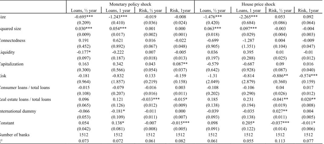
We estimate the model with OLS and apply heteroscedasticity-robust standard errors. All explanatory variables (except for the dummy variables) are demeaned for the regressions. The constant can therefore roughly be interpreted as the average effect, and the coefficient estimates should be interpreted relative to the constant. Since the average reaction of loans to monetary policy and house price shocks is positive, a negative coefficient implies a lower reaction. Conversely, as the average reaction of risk to monetary policy and house price shocks is negative, a negative coefficient implies a stronger reaction. The regression results are presented in Table 6.

We expect that small banks are more affected by macroeconomic shocks than large banks because of lower net worth, lack of diversification, and funding difficulties (Diamond and Rajan 2006, Kashyap and Stein 2000). Our results confirm the findings of previous studies that lending by small banks increases by more than lending by large banks after expansionary monetary policy shocks. The impact of size levels off as banks grow large, as shown by the

negative squared term. Size has no significant impact on the risk response to monetary policy shocks. The effect of size in response to a positive house price shock mirrors its effect after monetary policy shocks, as suggested by financial accelerator models.

Improved access to liquidity should reduce banks’ exposure to shocks affecting funding

conditions (Diamond and Rajan 2006). Liquidity in fact has a negative and significant impact on the exposure of lending to monetary policy in the short run: More liquid banks expand lending by less in response to a decline in policy rates than less liquid banks. This negative relation vanishes in the more medium run. Liquidity has no significant impact on risk responses or after house price shocks.

Next, we account for the fact that internationalization of banks could affect their exposure to

shocks. If shocks at home and abroad are imperfectly correlated, the presence of foreign affiliates might activate a channel of diversification, thereby reducing the response to domestic shocks. Cetorelli and Goldberg (2008) show that internationally oriented banks have the potential to lay off domestic macroeconomic shocks through linkages to their foreign affiliates, which reduces the exposure to domestic monetary policy shocks. We find that internationalization reduces banks’ lending response after one year, consistent with Cetorelli and Goldberg (2008), but it is not an important determinant in the short run. Banks possibly need some time to activate the internal capital market. Also, internationalization dampens the reaction of bank risk after a house price shock which might reflect better portfolio diversification of international banks.

Closer linkages between banks, measured as banks’ exposure to the interbank market can be

expected to increase the exposure to macroeconomic shocks (see Allen and Gale 2001). Yet, the degree of interconnectedness has no significant impact.

Risk, capitalization, or the exposure to real estate and consumer loans do not affect the

lending response of banks.22 But these variables affect the risk response. Exposure to the real estate market significantly amplifies the effect of monetary policy and house price shocks within the first four quarters. One explanation is that, after a monetary tightening, a decline in inflation increases the real value of debt obligations by borrowers and limits resources available to borrowers (Gerali et al. 2010). Additionally, negative second round asset price effects reduce collateral value. Moreover, we find a significantly positive effect of the degree of capitalization on the impact of monetary policy shocks on bank risk and a strong negative influence of riskiness on the impact of house price shocks on bank risk.

Overall, the lending response of smaller and not very liquid banks to expansionary monetary policy shocks is stronger than that for larger and more liquid banks. In the medium run, banks with foreign affiliates react less strongly to monetary policy shocks in terms of lending. Risk declines by more for banks highly engaged in real estate lending and for riskier banks, while better capitalized banks react less in terms of risk to monetary policy shocks. Moreover, lending of larger banks increases less in response to house prices shocks. Riskier banks react more to house price shocks while international banks react less in terms of risk.

5 Summary of Results and Policy Implications

In this paper, we use a FAVAR model to analyze feedback effects between banks and the macroeconomy. We focus on the heterogeneous exposure of over 1,500 U.S. banks to

22

This is in contrast to Kishan and Opiela (2000) and Gambacorta and Mistrulli (2004) who find that capitalization is an important determinant of banks ability to shield their loan portfolio from a tightening of monetary policy.

macroeconomic factors. There is no consensus in the theoretical and empirical literature on the effect of macroeconomic shocks on bank risk, and we make several contributions to the literature. First, we model the dynamic interaction of macroeconomic and banking factors. Second, we allow for and exploit the linkages between individual banks and between different banking variables such as banks’ risk and return. Third, we identify orthogonal macroeconomic shocks to cleanly decompose banks’ common risk into its different sources, and we isolate these shocks from idiosyncratic risk at the bank level.

We are now in the position to answer the questions raised at the beginning of the paper.

(i) How are macroeconomic shocks transmitted to bank risk and other banking variables?

Macroeconomic shocks have an important impact on bank risk and on other bank-level variables. Average bank lending increases following expansionary shocks, consistent with an increased demand for loans to finance investment and working capital during boom periods or an increased credit supply. Average bank risk declines after expansionary macroeconomic shocks with the exception of supply shocks. As a by-product we find that shocks to the banking factors matter for the macroeconomy, especially in the medium term when they explain more than 20 percent of macroeconomic volatility. Their explanatory power is largest for the monetary policy interest rate and for house prices. Omitting bank-level information can alter estimates of impulse responses and monetary policy shocks.

(ii) What are the sources of bank heterogeneity, and what explains differences in individual banks’ responses to macroeconomic shocks?

We find a substantial degree of heterogeneity across banks both in terms of idiosyncratic shocks and the asymmetric transmission of common (banking and macroeconomic) shocks. While average risk declines, risk of about 1/3 of all banks rises in response to a monetary loosening. We have also studied which bank-level features can explain differences in banks’ exposure to expansionary monetary policy shocks. Lending of small, not very liquid, and of domestic banks increases by more; risk of banks with a low degree of capitalization and a high exposure to the real estate market decreases to a relatively strong extent. As concerns the exposure to house price shocks we find that lending of larger banks increases less while risk of riskier and domestic banks reacts more after expansionary house price shocks.

Our findings are interesting from a banking regulation perspective. The result that less liquid and not well capitalized banks react more to macroeconomic shocks support proposals requiring more capital and higher liquidity ratios if regulators are concerned that the banking sector acts as an accelerator of macroeconomic shocks. At the same time, we find that small and purely domestic banks are more vulnerable to macroeconomic shocks. But one should also take into account that the systemic impact of these banks on the macroeconomy is rather small. Regulatory policy would therefore need to balance different criteria (the relevance of

an institution for systemic risk and its exposure to macroeconomic shocks) when deciding upon new capital or liquidity requirements.

In terms of future research, there are three additional issues which we consider promising. First, it would be interesting to disentangle domestic and global macroeconomic shocks and to assess if internationally active banks are worse off after adverse global shocks. Second, non-linearities, e.g. in the reaction of banks to common (macroeconomic and banking) shocks, may be present in exceptional situations such as banking crises. Our model has to be seen as suitable to analyze macro-banking feedbacks in “normal” times, but could be extended to allow for non-linearities. Third, the role of shocks to large banks for macroeconomic dynamics would be worth examining in details.

Overall, our analysis can be seen as a first step into the direction of jointly modeling dynamics of the banking sector and the macroeconomy. They suggest that these feedback effects are relevant for both, understanding macroeconomic dynamics as well as the behavior of banks. Research of this type would certainly benefit from high-quality microeconomic panel data.

6 References

Allen, F. and D. Gale (2001). Financial Contagion. Journal of Political Economy 108(1):

1-33.

Allen, F. and D. Gale (2004). Competition and Financial Stability. Journal of Money, Credit and Banking 36(3): 453-80.

Altunbas, Y., L. Gambacorta, D. Marqués Ibañez (2009). An Empirical Assessment of the Risk-Taking Channel. University of Wales, Bank for International Settlements, and European Central Bank. Mimeo. Basel.

Angeloni, I., and E. Faia (2009). A Tale of Two Policies: Prudential Regulation and Monetary Policy with Fragile banks. Kiel Institute for die World Economy. Kiel Working Paper 1569. Kiel.

Angeloni, I., E. Faia, M. Lo Duca (2010) Monetary Policy and Risk Taking, University of Frankfurt, Mimeo.

Bai, J. and S. Ng (2002). Determining the Number of Factors in Approximate Factor Models.

Econometrica 70(1): 191-221.

Bai J. and P. Perron (2003). Computation and Analysis of Multiple Structural Change Models. Journal of Applied Econometrics 18: 1-22.

Basel Committee on Banking Supervision (2009). Consultative proposals to strengthen the resilience of the banking sector announced by the Basel Committee. 17.12.2009. Basel.

Beck, G., K. Hubrich, and M. Marcellino (2009). Regional Inflation Dynamics within and across Euro Area Countries and a Comparison with the US. Economic Policy 57:

141-184.

Beck, T. (2008). Bank Competition and Financial Stability: Friends or Foes? World Bank Policy Research Working Paper 4656. Washington DC.

Berger, A. and T. Hannan (1991). The Rigidity of Prices: Evidence from the Banking Industry. American Economic Review 81(4): 938-45.

Berger, A. and C. Bouwman (2009). Bank Liquidity Creation. Review of Financial Studies

22(9): 3779-3837

Bernanke, B., M. Gertler, and S. Gilchrist (1996). The Financial Accelerator and the Flight to Quality. The Review of Economics and Statistics 78(1): 1-15.

Bernanke, B.S., J. Boivin, and P. Eliasz (2005). Measuring the Effects of Monetary Policy: A Factor-Augmented Vector Autoregressive (FAVAR) Approach. Quarterly Journal of Economics (February): 387-422.

Bjørnland, H., and D. H. Jacobsen (2008). The Role of House Prices in the Monetary Policy Transmission Mechanism in the US. Norges Bank Working Paper 2008/24. Oslo. Bloom, N. (2009). The Impact of Uncertainty Shocks. Econometrica 77(3): 623-685.

Boivin, J. and S. Ng (2006). Are more data always better for factor analysis? Journal of Econometrics 132(1): 169-194.

Boivin, J. and M. P. Giannoni (2007). Global Forces and Monetary Policy Effectiveness. National Bureau of Economic Research (NBER). Chapters, in: International Dimensions of Monetary Policy: 429-478. Cambridge, MA.

Boivin, J., M. Giannoni, and I. Mihov (2009). Sticky Prices and Monetary Policy: Evidence from Disaggregated US Data. American Economic Review 99(1): 350-84.

Borio, C., and H. Zhu (2008). Capital Regulation, Risk-Taking and Monetary Policy: A Missing Link in the Transmission Mechanism?. Bank for International Settlements Working Paper, No. 268. Basel.

Boyd, J. H. and G. De Nicoló (2005), The Theory of Bank Risk Taking and Competition Revisited. The Journal of Finance 60: 1329–1343.

Brunnermeier, M.K. (2008). Deciphering the Liquidity and Credit Crunch 2007-2008. Bureau of Economic Research (NBER). Working Paper 14612. Cambridge, MA.

Canova, F., and G. De Nicoló (2003). On the Sources of Business Cycles in the G-7. Journal of International Economics, Elsevier 59(1): 77-100.

Cetorelli, N. and L. S. Goldberg (2008). Banking Globalization, Monetary Transmission, and the Lending Channel. National Bureau of Economic Research (NBER), Working Paper 14101, Cambridge MA.

Chamberlain, G., and M. Rothschild (1983). Arbitrage, Factor Structure and Mean-Variance Analysis in Large Asset Markets, Econometrica, 51, 1305-1324.

Christiano, L. J., M. Eichenbaum and C. Evans (1996). The Effects of Monetary Policy Shocks: Evidence from the Flow of Funds. The Review of Economics and Statistics

78(1): 16-34.

Ciccarelli, M., A. Maddaloni, and J.-L. Peydró (2009). Trusting the Bankers: A New Look at the Credit Channel of Monetary Policy. European Central Bank. Mimeo. Frankfurt a.M.

Dave, C., S.J. Dressler, and L. Zhang (2009). The Bank Lending Channel: a FAVAR Analysis. University of Texas at Dallas, Villanova University. Mimeo.

Del Negro, M., and C. Otrok (2007). 99 Luftballons: Monetary Policy and the House Price Boom Across States, Journal of Monetary Economics, 54, 1962-1985.

Den Reijer, A.H.J. (2007). Identifying Regional and Sectoral Dynamics of the Dutch Staffing Labour Cycle. DNB Working Paper 153.

De Nicoló, G., and M. Lucchetta (2010). Systemic Risk and the Macroeconomy. International Monetary Fund. IMF Working Paper 10/29. Washington DC.

De Graeve, F., T. Kick and M. Koetter (2008). Monetary policy and financial (in)stability: An integrated micro-macro approach. Journal of Financial Stability 4(3): 205-231.

Dell’Ariccia, G., and R. Marquez (2006). Lending Booms and Lending Standards. The Journal of Finance LXI(5): 2511-2546.

Diamond, D. W. and R. G. Rajan, (2006). Money in a Theory of Banking. American Economic Review 96(1): 30-53.

Dib, A (2010). Banks, Credit Market Frictions, and Business Cycles. mimeo

Eickmeier, S. (2009). Comovements and Heterogeneity in the Euro Area Analyzed in a Non-Stationary Dynamic Factor Model. Journal of Applied Economics 24(6): 933-959.

Eickmeier, S., B. Hofmann, and A. Worms (2009). Macroeconomic Fluctuations and Bank Lending: Evidence for Germany and the Euro Area. German Economic Review 10(2):

193-223.

Eickmeier, S., and B. Hofmann (2010). Housing Booms, Financial (Im)Balances and Monetary Policy. ECB Working Paper 1178 and Bundesbank Discussion Paper (Series 1), 07/2010. Frankfurt a.M.

Farhi, E., and J. Tirole (2009). Collective Moral Hazard, Maturity Mismatch and Systemic Bailouts. National Bureau of Economic Research (NBER). Working Paper 15138. Cambridge, MA.

Frankel, J, and G. Saravelos (2010). Are Leading Indicators of Financial Crises Useful for Assessing Country Vulnerability? Evidence from the 2008-09 Global Crisis. National Bureau of Economic Research (NBER). Working Paper 16047. Cambridge, MA. Fry, R. and A. Pagan (2007). Some Issues in Using Sign Restrictions for Identifying

Structural VARs. National Center for Economic Research (NCER). Working Paper 14. Canberra.

Gambacorta, L. and P. E Mistrulli,. (2004).Does bank capital affect lending behavior?

Gambarcorta, L. (2009). Monetary Policy and the Risk-Taking Channel. BIS Quarterly Review. December: 43-53. Basel.

Gerali, A., S. Neri, L. Sessa, F. M. Signoretti (2010). Credit and Banking in a DSGE Model of the Euro Area. Journal of Money, Credit and Banking 42: 107–141.

Gersbach, H., and V. Hahn (2009). Banking-on-The-Average Rules. CER-ETH - Center of Economic Research at ETH Zurich. Working Paper No. 09/107. Zurich.

Goel, Anand M., Fenghua Song, and Anjan V. Thakor (2009). Infectious Leverage. Federal Reserve Bank of Chicago, Pennsylvania State University, and Washington University. Mimeo.

Hellwig, M. (1997). Banks, Markets, and the Allocation of Risks in an Economy. Sonderforschungsbereich 504 Publications 97-35, Sonderforschungsbereich 504, Universität Mannheim & Sonderforschungsbereich 504, University of Mannheim. Hellwig, M. (2009).Systemic Risk in the Financial Sector: An Analysis of the

Subprime-Mortgage Financial Crisis. De Economist 157(2): 129-207.

International Monetary Fund (IMF) (2009). Global Financial Stability Report. April.

Washington DC.

Ioannidou, V., Ongena, S. and Peydro, J.L., (2009).Monetary Policy, Risk-Taking, and Pricing: Evidence from a Quasi-Natural Experiment. Discussion Paper 2009-31 S, Tilburg University, Center for Economic Research.

Jarociński, M., and F. Smets (2008). House Prices and the Stance of Monetary Policy.

Federal Reserve Bank of St. Louis Review 90(4): 339-65.

Jiménez, G., S. Ongena, J.L. Peydró, and J. Saurina (2007). Hazardous Times for Monetary Policy: What Do Twenty-Three Million Bank Loans Say About the Effects of Monetary Policy on Credit Risk. Bank of Spain, ECB, and Tilburg University. Mimeo.

Kashyap, A. K., and J. C. Stein (2000). What Do a Million Observations on Banks Say about the Transmission of Monetary Policy? American Economic Review 90(3): 407-428.

Kilian, L. (1998).Small-Sample Confidence Intervals For Impulse Response Functions. The Review of Economics and Statistics 80(2): 218-230.

Kishan, R. P. and T. P Opiela (2000). Bank Size, Bank Capital, and the Bank Lending Channel. Journal of Money, Credit and Banking 32(1): 121-41.

King, T. B. (2008). Discipline and Liquidity in the Interbank Market. Journal of Money, Credit and Banking 40(2-3): 295-317.

Kiyotaki, N. and Moore, J. (1997). Credit Cycles. Journal of Political Economy 105(2):

211-48.

Kose, A., C. Otrok, and C.H. Whiteman (2003). International Business Cycles: World, Region and Country Specific Factors. American Economic Review 93(4): 1216-1239.

Martínez-Miera, D., and R. Repullo (2010). Does Competition Reduce the Risk of Bank Failure? Review of Financial Studies 23(10): 3638-3664.

Matsuyama, K. (2007). Credit Traps and Credit Cycles. American Economic Review 97(1):

503-516.

Meh, C., and K. Moran (2010). The Role of Bank Capital in the Propagation of Shocks.

Journal of Economic Dynamics and Control 34: 555-576.

Mönch, E., S. Ng, and S. Potter (2009). Dynamic Hierarchical Factor Models, Federal Reserve Bank of New York Staff Reports. 412 December. New York.

Otrok, C., and P.M. Pourpourides (2008). On the Cyclicality of Real Wages and Wage Differentials. Mimeo. University of Virginia.

Peersman, G. (2005). What Caused the Early Millennium Slowdown? Evidence based on Vector Autoregressions. Journal of Applied Econometrics 20(2): 185-207.

Rajan, R.G. (2005). Has Financial Development Made the World Riskier? National Bureau of Economic Research (NBER). Working Paper 11728. Cambridge, MA.

Rochet, J.-C. (2008). Macroeconomic Shocks and Banking Supervision. In: Rochet, Why are there so many banking crises? The Politics and Policy of Bank Regulation.

Rubio-Ramírez, J.F., D.F. Waggoner, T. Zha (2010). Structural Vector Autoregressions: Theory of Identification and Algorithms for Inference Review of Economic Studies

77(2): 665-696.

Stock, J. H. and M.W. Watson (1998). Diffusion indexes. NBER Working Paper 6702. Stock, J. H. and M.W. Watson (2002). Macroeconomic Forecasting using Diffusion Indexes.

Journal of Business and Economic Statistics 20(2): 147-162.

Stock, J. H. and M. W. Watson (2005). Implications of Dynamic Factor Models for VAR Analysis. National Bureau of Economic Research (NBER). Working Paper 11467. Cambridge, MA.

Taylor, J. (2009). The Financial Crisis and the Policy Responses: An Empirical Analysis of What Went Wrong. NBER Working Paper 14631.

Uhlig, H. (2005). What are the Effects of Monetary Policy on Output? Results from an Agnostic Identification Procedure. Journal of Monetary Economics 52: 381-419.

Walsh, Carl E. (2003). Monetary Theory and Policy (2nd edition). The MIT Press

(Cambridge MA).

Zhang, L. (2009). Bank Capital Regulation, the Lending Channel, and Business Cycles. Deutsche Bundesbank. Discussion Paper Series 1: Economic Studies. 33/2009. Frankfurt a.M.