Title
Developing Intensity-Duration-Frequency (IDF) Curves From Satellite-Based Precipitation:
Methodology and Evaluation
Permalink
https://escholarship.org/uc/item/3n2558w1
Journal
WATER RESOURCES RESEARCH, 54(10)
ISSN
0043-1397
Authors
Ombadi, Mohammed
Nguyen, Phu
Sorooshian, Soroosh
et al.
Publication Date
2018-10-01
DOI
10.1029/2018WR022929
License
https://creativecommons.org/licenses/by/4.0/ 4.0
Peer reviewed
Developing Intensity-Duration-Frequency (IDF) Curves From
Satellite-Based Precipitation: Methodology and Evaluation
Mohammed Ombadi1 , Phu Nguyen1,2, Soroosh Sorooshian1 , and Kuo-lin Hsu1,3
1
Center for Hydrometeorology and Remote Sensing, Department of Civil and Environmental Engineering, University of California, Irvine, CA, USA,2Department of Water Management, Nong Lam University, Ho Chi Minh City, Vietnam,3Center for Excellence for Ocean Engineering, National Taiwan Ocean University, Keelung, Taiwan
Abstract
Given the continuous advancement in the retrieval of precipitation from satellites, it is important to develop methods that incorporate satellite-based precipitation data sets in the design and planning of infrastructure. This is because in many regions around the world, in situ rainfall observations are sparse and have insufficient record length. A handful of studies examined the use of satellite-based precipitation to develop intensity-duration-frequency (IDF) curves; however, they have mostly focused on small spatial domains and relied on combining satellite-based with ground-based precipitation data sets. In this study, we explore this issue by providing a methodological framework with the potential to be applied in ungauged regions. This framework is based on accounting for the characteristics of satellite-based precipitation products, namely, adjustment of bias and transformation of areal to point rainfall. The latter method is based on previous studies on the reverse transformation (point to areal) commonly used to obtain catchment-scale IDF curves. The paper proceeds by applying this framework to develop IDF curves over the contiguous United States (CONUS); the data set used is Precipitation Estimation from Remotely Sensed Information Using Artificial Neural Networks–Climate Data Record (PERSIANN-CDR). IDFs are then evaluated against National Oceanic and Atmospheric Administration (NOAA) Atlas 14 to provide a quantitative estimate of their accuracy. Results show that median errors are in the range of (17–22%), (6–12%), and (3–8%) for one-day, two-day and three-day IDFs, respectively, and return periods in the range (2–100) years. Furthermore, a considerable percentage of satellite-based IDFs lie within the confidence interval of NOAA Atlas 14.Plain Language Summary
Intensity-duration-frequency (IDF) curves are used for the design of infrastructure. At any specific location, the rainfall intensity can be obtained for a given duration and frequency of occurrence (known as return period). Development of IDF curves is based on probabilistic analysis of past records of extreme rainfall. However, in many regions around the world, particularly in developing countries, such records are not available either due to limited spatial coverage of ground rainfall gauges, short record length, or poor data quality. Satellite-based precipitation is an alternative source that can be utilized to develop IDF curves since it has near global coverage and high spatiotemporal resolution. In this paper, we explore the use of satellite-based precipitation products in developing IDF curves by providing a framework that accounts for the characteristics of satellite-based precipitation. Furthermore, we develop IDF curves for the contiguous United States (CONUS) and evaluate them using National Oceanic and Atmospheric Administration (NOAA) Atlas 14 as a benchmark. The results demonstrate that IDFs derived from satellite-based precipitation are of good accuracy. The methods used in this study have the potential to be extended and applied in other regions in the absence of in situ rainfall observations.1. Introduction
Engineering design of infrastructure requires information about runoff magnitudes for which the structures will be designed to withstand during their lifetime. In order to estimate these magnitudes, intensity (depth) duration frequency—IDF (DDF)—curves are the typical input to hydrological models used by hydrologists and civil engineers for design purposes. They represent a mathematical relationship between frequency, duration, and intensity (depth) of rainfall events. Their accuracy is contingent upon input data quality and sta-tistical inference methods. The concept of the IDF dates back to the efforts of Bernard (1932) and since then many studies have focused on improving statistical inference methods used in IDF development. Most nota-ble are the studies of Hosking and Wallis (1997) of introducing L-moments estimation (see also Hosking, 1990), the use of probability weighted moments estimation (Greenwood et al., 1979; Landwehr et al., 1979), parametric formulation of IDF relationships (Koutsoyiannis et al., 1998), and implementing
RESEARCH ARTICLE
10.1029/2018WR022929 Key Points:
• A methodological framework to develop IDF curves from satellite-based precipitation is presented
• The framework is implemented to develop IDFs over the contiguous United States, which are evaluated using NOAA Atlas 14 as a benchmark
• Results demonstrate the high potential of using satellite-based precipitation to develop IDF curves in data scarce regions
Supporting Information: •Supporting Information S1 Correspondence to: M. Ombadi, mombadi@uci.edu Citation:
Ombadi, M., Nguyen, P., Sorooshian, S., & Hsu, K. (2018). Developing intensity-duration-frequency (IDF) curves from satellite-based precipitation: Methodology and evaluation.Water Resources Research,54, 7752–7766. https://doi.org/10.1029/2018WR022929
Received 12 MAR 2018 Accepted 28 AUG 2018 Accepted article online 4 SEP 2018 Published online 16 OCT 2018
©2018. American Geophysical Union. All Rights Reserved.
regionalization methods such as the Index Flood method (Dalrymple, 1960; Hosking & Wallis, 1993; Wallis, 1982). Today, atlases of IDF curves have already been developed for several developed countries; an example of such efforts is National Oceanic and Atmospheric Administration (NOAA) Atlas 14 developed by the National Weather Service (NWS) at National Oceanic and Atmospheric Administration (NOAA; Bonnin et al., 2006, 2011; Perica et al., 2011, 2013a, 2013b), which succeeded NOAA Atlas 2 developed in 1973.
Despite the aforementioned methodological advancements in IDF formulation, construction of IDF curves for most countries around the world remains a major challenge. This is mainly because of the limited availability of long rainfall records with adequate spatial distribution to reflect temporal variation and spatial heteroge-neity of precipitation. As has been stated earlier, the accuracy of IDF curves is dependent on both input data quality and statistical inference methods. While considerable research focus has been given to the latter, only a handful of studies examined the former. Some of these studies investigated the use of alternative sources of rainfall measurements such as radar (Eldardiry et al., 2015; Marra et al., 2017; Marra & Morin, 2015; Overeem et al., 2008), satellite-based precipitation, or downscaled global climate model’s simulations of precipitation (DeGaetano & Castellano, 2017). Regarding the use of satellite-based precipitation, Endreny and Imbeah (2009) utilized Tropical Rainfall Measuring Mission (TRMM) rainfall data set in combination with rainfall data from ground gauges to construct IDF curves over Ghana. Similarly, Awadallah et al. (2011) investigated the use of TRMM and ground-based rainfall data to develop IDF curves over a region in Northwestern Angola. Recently, Gado et al. (2017) used the PERSIANN-CDR data set to develop IDF curves in ungauged sites by com-bining ground gauge data from neighboring sites in two basins in Colorado and California. Meanwhile, Marra et al. (2017) used Climate Prediction Center morphing (CMORPH) data to develop IDF curves over the eastern Mediterranean and compared them to IDF derived from radar data. Overall, these studies highlighted the benefit of using satellite-retrieved precipitation as an alternative source, particularly in partially gauged sites. However, several reasons limit the adequacy of these studies and the extension of their application to other regions. First, the methods used in most of these studies strongly rely on the partial availability of rainfall data sets with sufficient record length from ground gauges in the site of interest or in their neighboring sites, which is not satisfied in many regions. Second, they approached the use of satellite-based precipitation in IDF development from a case-study perspective and focused on small-scale regions; therefore, it is uncertain whether these methods will provide adequate results in regions with different climatic and precipitation regimes. Finally, and most importantly, the results of these studies were either not evaluated or evaluated in a small-scale domain. In other words, it is unknown whether these results underestimate or overestimate IDF curves that would ideally be derived from a dense network of rainfall gauges data.
In light of the aforementioned issues associated with previous studies on the use of satellite-based precipita-tion to develop IDF curves, the overarching goal of this article is to provide a methodological framework for developing IDF curves from satellite-based precipitation. This is achieved by,first, considering and analyzing the systematic error component (i.e., bias) in extreme satellite-retrieved precipitation; second, considering the necessary transformation of satellite-based precipitation from an area averaged to point rainfall; and
finally, the application of commonly used regionalization methods to derive IDF curves. The area-to-point transformation implied in this framework is based on previous research studies that focused on the reverse transformation (i.e., point-to-area). The paper proceeds by applying this framework to develop IDF curves of durations one, two, and three days over the contiguous United States (CONUS). While this research was moti-vated by the potential of using satellite-based precipitation to develop IDF curves in data-scarce regions, CONUS has been chosen as a test bed because of the availability of rigorous IDF estimates from ground gauges provided by NOAA Atlas 14. Therefore, IDF curves derived from satellite-based precipitation are eval-uated and compared to NOAA Atlas 14 to assess the performance of the framework.
The subsequent sections of this article are organized as follows. Section 2 presents the data sets used in this study as well as describing the case study region and its geographic sections. In section 3, a detailed descrip-tion of the methodological framework for developing IDF curves is provided. This secdescrip-tion includes the ana-lysis of systematic error in extreme satellite-based precipitation, a model for bias adjustment of extreme satellite-based precipitation, and a method to transform areal rainfall to point rainfall. Section 4 provides the results and their evaluation as well as an analysis of their uncertainty. The paper concludes in section 5 by highlighting the mainfindings and discussing issues that need to be explored thoroughly and that might be the focus of future research studies.
2. Data and Case Study
2.1. PERSIANN-CDRThe satellite-based precipitation data set used in this study to derive IDF curves is Precipitation Estimation from Remotely Sensed Information using Artificial Neural Networks–Climate Data Record (PERSIANN-CDR; Ashouri et al., 2015). This data set has daily temporal resolution, spatial resolution of (0.25° × 0.25°), and near global coverage (60°S–60°N) for the period (1983 to present). PERSIANN-CDR is based on infrared (IR) imagery from geostationary satellites, and it is a unique data set because of its relatively long record (1983 to delayed present) compared to other satellite-based precipitation products. Other satellite-based precipitation products that can potentially be utilized for the development of IDF curves include the CMORPH (Joyce et al., 2004) and TRMM Multisatellite Precipitation Analysis (TMPA; Huffman et al., 2007). Both products have high temporal resolution of 3 hr and a spatial resolution of (0.25° × 0.25°). CMORPH record covers the period (2002 to present); meanwhile, TMPA is available for the period (1998–2015). In this study, we opted to select PERSIANN-CDR pri-marily because of its relatively long record.
Although in this study IDF curves have been solely derived from PERSIANN-CDR, two secondary data sets were used. First, Climate Prediction Center (CPC) Unified Gauge-Based Analysis of Daily Precipitation over CONUS, hereafter referred to as CPC, has been used to estimate parameters of the bias adjustment model. Second, the NOAA Atlas 14 data set has been used as a basis for the evaluation of IDF curves derived from satellite-based precipitation.
2.2. CPC Unified Gauge-Based Analysis of Daily Precipitation Over CONUS
The CPC data set was developed by NOAA’s CPC. It covers the period (1948 to present) and has a similar spa-tial resolution to PERSIANN-CDR (0.25° × 0.25°). However, in this study, only CPC record in the period (1983 to present; i.e., same time coverage as PERSIANN-CDR) has been used. CPC data set was produced from a dense gauge network over the CONUS with approximately 8,500 stations and a mean station-to-station distance of ~30 km (Chen et al., 2008). The interpolation algorithm used to develop the products is the Optimal Interpolation (OI) method (Gandin, 1965); this method proved to be reliable and provides results with high correlation in several studies (Chen et al., 2008; see also Bussieres & Hogg, 1989; Creutin & Obled, 1982). 2.3. NOAA Atlas 14
The NOAA Atlas 14 data set was developed by NOAA’s National Weather Service (NWS; Bonnin et al., 2006, 2011; Perica et al., 2011, 2013a, 2013b), and it is not yet available for the states of Texas, Oregon, Washington, Idaho, Montana, and Wyoming. NOAA Atlas 14 over CONUS is divided intofive geographic regions as shown in Figure 1; these geographic regions have been adopted in this study for evaluation pur-poses since they represent, to some extent, regions with distinct climatic and precipitation regimes. NOAA Atlas 14 is derived from a dense network of rainfall gauges with an average record length range of (54–68) years (Bonnin et al., 2006, 2011; Perica et al., 2011, 2013a, 2013b).
3. Methodology
3.1. Bias in Satellite-Based Extreme Precipitation
In recent decades, a multitude of studies have been devoted to the evaluation of satellite-retrieved precipita-tion (e.g., AghaKouchak et al., 2011; Behrangi et al., 2011; Dinko et al., 2008; Ebert et al., 2007; Sorooshian et al., 2000). While these evaluation studies differ from each other in many aspects, such as geographic location over which the evaluation is performed, temporal scale (e.g., daily, monthly), and evaluation metrics, the consensus is that satellite-based precipitation exhibits errors, both random and systematic. Moreover, satellite-based precipitation products have lower skill in detecting heavy rainfall (Mehran & AghaKouchak,
Figure 1.Geographic regions of contiguous United States (CONUS) accord-ing to National Oceanic and Atmospheric Administration (NOAA)-Atlas 14 volumes (Volume 1 and 6: Semiarid Southwest and California, Volume 2: Ohio River Basin and Surrounding States, Volume 8: Midwestern States, Volume 9: Southeastern States and Volume 10: Northeastern States). Updating inten-sity-duration-frequency (IDF) curves for Texas is in progress, while updated IDF curves are unavailable for the states of Washington, Oregon, Idaho, Montana, and Wyoming.
2014). Therefore, it is necessary to examine errors in satellite-based preci-pitation prior to their use in IDF development.
As far as IDF studies are concerned, only extreme rainfall events, defined as events higher than the 99th percentile of the distribution of rainfall totals accumulated over a specific duration, are of importance. This is because both approaches commonly used to sample extreme events, namely, Annual Maximum Series (AMS) and Partial Duration Series (PDS), contain rainfall values that are typically higher than the 99th percentile. Hence, in this study, analysis of errors in PERSIANN-CDR is carried out as follows. First, AMS is extracted from both ground-based precipitation (CPC) and satellite-based precipitation (PERSIANN-CDR) data sets for each grid (0.25° × 0.25°); the AMS length is 33 years, and it is extracted from the per-iod of hydrological years (1984–2016). Second, an adjustment factor (ζ) is defined as the ratio of ground-based (CPC) to satellite-based precipitation (PERSIANN-CDR), that is:
ζðx;y;kÞ¼ RG x;y;kð Þ
RS x;y;kð Þ (1)
whereζ(x,y,k)is the adjustment factor for thekth event in the AMS at loca-tion (x,y),RG(x,y,k)is thekth ground-based rainfall event in the AMS at loca-tion (x,y), andRS(x,y,k)is thekth satellite-based rainfall event in the AMS at location (x,y). Next, at each grid location the average adjustment factorζð Þx;y of values in equation (1) is cal-culated; this factor represents the systematic error (i.e., bias) in extreme satellite-based precipitation. Figure 2 shows the relationship between elevation andζð Þx;y. It can be clearly seen that the bias is significantly correlated with elevation as indicated by Pearson’s correlation coefficient value of 0.54. This indicates that 29% (0.542) of the variability in the bias can be explained linearly by elevation. Hence, it can be concluded that, in general, satellite-based precipitation (PERSAINN-CDR) tends to have higher bias, particularly underes-timation bias, in high-altitude regions. The presence of this relationship in PERSIANN-CDR as well as other satellite-based precipitation products has been observed in previous studies (e.g., Hashemi et al., 2017; Miao et al., 2015). This is due to the fact that warm orographic rainfall over high-altitude regions poses a chal-lenge to satellite-based precipitation retrieval algorithms based on IR imagery (Dinko et al., 2008).
3.2. Bias Adjustment Model
Based on the previous analysis, the following model is proposed as a new approach to adjust extreme satellite-retrieved precipitation; the model utilizes elevation as the only explanatory variable.
ζð Þx;y ¼αeβEð Þx;y (2) whereEis elevation in meters,αandβare parameters, andζð Þx;y is defined as before.
Figure 2 (blue curve) shows the estimated adjustment factors based on the model for one-day annual max-imum series. Estimation of the model parameters can be carried out in a simple manner by recognizing that the model can be solved analytically by linearization. This can be performed by taking the natural logarithm of both sides in equation (2), then solving for the values of the parameters ln(α) andβusing ordinary least squares solution. It should be noted that the parametersαandβare estimated for each duration of interest (i.e., one day, two days, and three days) separately. Table 1 lists the values of parameters and their 95% confidence intervals for each duration of interest.
3.3. Transformation of Areal Rainfall to Point Rainfall
An important issue to be considered when developing IDF curves from satellite-based precipitation is the areal nature of the data, since all
Figure 2.Relationship between elevation (meters) and the adjustment fac-tor defined in equation (1) for annual maximum series of one day. The red dots represent observations, while the blue line represents the adjustment model calculated from equation (2) with the values of parameters given in Table 1.
Table 1
Values of the Bias Adjustment Model Parameters for Annual Maximum Series of Durations One, Two, and Three Days
One day Two days Three days
α 1.308 1.2557 1.2180
(1.3019–1.3142) (1.2497–1.2616) (1.2123–1.2238)
β 1.6627 × 10⁻⁴ 1.7978 × 10⁻⁴ 1.7865 × 10⁻⁴ (1.6186–1.7068) × 10
4 (1.7531–1.8424) × 104 (1.7418–1.8313) × 104 Note. Values in parenthesis are the 95% confidence bounds for the para-meters estimates.
products of satellite-based precipitation estimate the average precipi-tation depth over a grid area, which is in the case of PERSIANN-CDR is (25 km × 25 km = 625 km2). Areal rainfall distribution has both a lower mean and variance compared to the distribution of point rainfall; this follows directly from the fact that the former is an averaged random process of the latter. It is widely stated in the literature that in general the difference between the areal and point distributions increases with decrease in the total rainfall depth (Eagleson, 1970; Rodriguez-Iturbe & Mejía, 1974a). This is mainly because events that produce low amounts of rainfall tend to be more localized. This relationship is significantly present in satellite-based precipitation as shown in Figure 3. It can be clearly seen that high quantiles of rainfall depths correspond to low quantiles of bias (i.e., systematic error) with a Pearson’s correlation coefficient value of0.38.
Considerable research attention has been assigned to the develop-ment of methods that transform point IDF curves to areal IDF curves; such a transformation requires reduction factors commonly known as areal reduction factors (ARFs). Methods of developing ARFs fall into two categories:first, empirical methods which utilize rainfall time ser-ies data from gauge network in a specific region to develop relation-ships between point and area-averaged rainfall (e.g., U.S. Weather Bureau, 1957, 1958) and second, theory-based methods which are theory-based on the stochastic representation of rainfallfields in space and time. In this study, we adopt a theory-based approach to derive ARFs, which was proposed by Sivapalan and Blöschl (1998) and is based on the spatial correlation structure of the rainfallfield. It should be noted that contrary to the common use of ARFs, we are interested in transforming areal to point rainfall; thus, we will use the reci-procals of ARFs. The methodology consists offirst assuming an isotropic correlogram (i.e., spatial correlation structure) of point rainfall of the following exponential form:
ρð Þ ¼r expðr=λÞ (3) whereρis correlation,ris the Euclidean distance between two points, andλis a parameter that specifies the decay in correlation. To estimate the parameterλ, equation (3) has to befitted to preserve the mean observed correlation at a distance known as the characteristic distancerA(Rodriguez-Iturbe & Mejía, 1974a, 1974b); this distance is a function of the shape and size of the area under consideration. The characteristic distance (rA) is defined as the mean distance between two randomly chosen points in the region of interest, and its distribu-tion was provided by Ghosh (1951). Matérn (1986) used the distribudistribu-tion to compute the ratio of the charac-teristic to the maximum distances for unit areas with standard shapes (e.g., square and circle). The following result was found for a square unit area (A):
rA¼0:7374diagonal Að Þ (4)
Applying this result on the grids of PERSIANN-CDR (25 km × 25 km) will result in a characteristic distance of 26.07 km. However, because the distances between the grid centers for which equation (3) can be computed can only take multiples of 25 km (i.e., 25, 50, and 75), we have takenrAto be 25 km. Then, the average observed cross correlation between the annual maximum series at distances of 25 km was calculated for each of the geo-graphic sections shown in Figure 1. Finally, equation (3) isfitted to the values of observed correlations to estimate the value of parameter λ. Additionally, in order to evaluate the bias resulted from assigning a value of 25 km instead of 26.07 km to the characteristic distance, the sensitivity of the parameterλto changes in the characteristic distance have been investigated. The results (see Table 2) demonstrate that the sensitivity is different in each geographic region depending on the precipitation mechanism. However, the average sensitivity is in the order of 7.5% for a
Figure 3.Density plot for the joint distribution of one-day annual maximum series rainfall quantiles and error quantiles; quantiles are calculated using the Weibull plotting position. Data used to plot the density include all grids over the contig-uous United States (CONUS).
Table 2
Percentage Change in the Estimate of ParameterλResulting From Changes in the Characteristic Distance of 25, 50, and 75 km
25 km (%) 50 km (%) 75 km (%) Southwestern States 8.4 16.04 21.5 Southeastern States 4.95 6.6 7.6 Northeastern States 19.87 26.56 40.23 Ohio River Basin 2.88 4.0 6.3 Midwestern States 1.46 1.8 2.13
change of 25 km in the characteristic distance and it increases consistently with more significant changes in the characteristic distance. Therefore, the bias in the parameterλresulted from assigning a value of 25 km instead of 26.07 km is on average significantly less than 7.5%.
After estimating the parameterλ, the variance reduction factorκ2, defined as the expectation of the correlation between any two random points within the region under consideration, can be calculated according to the following equation (Rodriguez-Iturbe & Mejía, 1974a; Sivapalan & Blöschl, 1998):
κ2¼E ρ x 1x2
ð Þ
½ (5)
Furthermore, Rodriguez-Iturbe and Mejía (1974a) showed that equation (5) can be simplified by integrating the product of the probability density function of variablerand the correlation function according to the follow-ing equation:
κ2¼∫diagð ÞA
0 ρð Þr fRð Þr : dr (6) whereρandris defined as above andfR(r) is the probability density func-tion of the random variabler. For a square area with side lengtha(e.g., in the case of PERSIANN-CDR,a= 25 km), Ghosh (1951) has derived the distribution ofr(i.e.,fR(r)).
fRð Þ ¼r 4r a4 1 2πa 22arþ1 2r 2 ; 0≤r≤a 4r a4 sin 1a ra 2cos1a rþ2a ffiffiffiffiffiffiffiffiffiffiffiffiffiffi r2a2 p 12r2þ2a2 ; a≤r≤pffiffiffiffiffi2a 8 > > > < > > > : (7)
Thefinal step is to use the variance reduction factor estimated from equation (6) to adjust the parameters of the generalized extreme value (GEV) probability distribution that will befitted to the data according to equa-tions (8) and (9). These equaequa-tions have been derived by Sivapalan and Blöschl (1998) by matching the para-meters of areal and point extreme rainfall distributions in the particular case of zero area. See Sivapalan and Blöschl (1998) for detailed derivation of equations (8) and (9).
μp¼ μA κ2ð0:39þ0:61κ1:6Þ (8) αp¼ αA 10:17 lnðκ2Þ ð Þ κ2 (9)
whereμpandμAare the point and areal GEV distribution location parameters, respectively; similarlyαpandαA are the point and areal scale parameters, respectively.
This theory-based approach to derive area-to-point transformation factors has been validated in Sivapalan and Blöschl (1998). The validation was performed by comparing the ARFs derived by this method to ARFs observed in actual storms. In this study, we investigated the validity of the methodology by examining an extreme rainfall event over Texas on 27 August 2018 associated with hurricane Harvey. Total 24-hr rainfall was obtained from NCEP Stage IV multisensor (i.e., radar and gauges) precipitation data, then the observed ARFs were calculated (red line with markers in Figure 4). Next, using one-day IDF estimates for that region reported in Cleveland et al. (2015), the observed ARFs were matched through the selection of appropriate correlation lengthλ. Further details of the validation process such as the equations used for the selection of appropriate correlation length are provided in Text S1. Figure 4 demonstrates that the two enveloping curves for the observed ARFs correspond to correlation lengths of 120 and 160 km. Since the correlation length reflects information about the rainfall generating mechanism, these large values of correlation length are consistent with the large synoptic-scale event that produced this storm. It should be noted that this is an approximate validation since the observed ARFs are storm-centered (i.e., specific to storm); meanwhile, the simulated ARFs arefixed-area ARFs.
Figure 4.Observed Area Reduction Factors (ARFs; red line with markers) and estimated ARFs by the proposed methodology (blue lines) for an extreme rainfall event on 27 August 2018 over Texas associated with hurricane Harvey.
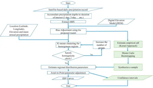
3.4. Developing IDF Curves
After adjusting the bias in the annual maximum series extracted from PERSIANN-CDR using the model described in section 3.2, the process of developing IDF curves is carried out in several steps illustrated in Figure 5. First, regionalization is applied to improve the statistical inference by increasing the number of samples. This is achieved by creating homogenous regions using the k-means algorithm to cluster grids. This step starts with input data to the algorithm that constitute latitude, longitude, elevation, and mean annual precipitation; these data to a certain extent define different climatic divisions. Next, the output clusters from the k-means algorithm are tested statistically for homogeneity using the method described in Hosking and Wallis (1993). In this method the within-cluster variation in L-CV (i.e., the ratio of second to
first L-moments) is compared with what would be expected by simulations from a general probability
Figure 5.Flowchart illustrates the process of developing intensity-duration-frequency (IDF) curves from satellite-based precipitation. Processes in green illustrate generally the process of estimating confidence intervals.
Figure 6.Q-Q plot comparing the quantiles of AMS extracted from Climate Prediction Center (CPC; horizontal axis) and Annual Maximum Series (AMS) extracted from Precipitation Estimation from Remotely Sensed Information Using Artificial Neural Networks–Climate Data Record (PERSIANN-CDR; vertical axis) at (a) (37.625°N, 119.375°W), California, altitude = 3272 m and (b) (37.625°N, 78.125°W), Virginia, altitude = 96 m. The red dots and line represent the quantiles before adjustment and its linearfit. Similarly, the blue dots and line represent the quantiles after adjustment and its linear fit. The gray dotted line represents the equality line (x=y).
distribution; in this study the Wakeby distribution (Houghton, 1978; see also Hosking & Wallis, 1997) was used. If clusters are not satisfactory according to the homogeneity check, clustering is repeated with increas-ing the number of groups. It should be noted that clusterincreas-ing might be different for each duration of interest (e.g., one day and two days) since it depends on L-CV values of each AMS.
Following the identification of homogenous regions, the AMS at each grid is normalized by dividing it by the mean AMS value. Then, the AMSs in each homogenous region are combined andfitted to a GEV distribution. The choice of the GEV distribution to model the extreme rainfall process was validated using the Kolmogorov-Smirnov test (Massey, 1951); results showed that GEV is an adequate distribution to represent the annual max-imum series. The location and scale parameters of the distribution are then adjusted to account for the transformation of areal to point rainfall using the approach described in section 3.3.
Finally, precipitation quantiles corresponding to return periods (2, 5, 10, 25, 50, and 100) years are calculated using the indexflood procedure (Hosking & Wallis, 1997). In this approach, the quantiles for each homoge-nous region, also known as the regional growth factors, are estimated. Next, to account for normalization, the quantiles in each grid cell are calcu-lated by multiplying the mean AMS value at the cell by the growth factor according to the following equation:
qð Þx;y ¼μð Þx;ybq (10)
whereq(x,y)is the quantile at grid (x,y),μ(x,y)is the mean of AMS at grid (x,y), andbqis the regional growth factor for the homogenous region of interest.
3.5. Estimation of Confidence Intervals
Confidence intervals are estimated using Monte Carlo bootstrapping; the method consists of three steps. First, the at-site empirical cumula-tive distribution function is estimated at each grid cell center using Kernel density estimation (Parzen, 1962; Rosenblatt, 1956). Second, samples of AMS are extracted from the empirical distribution with the same length of record as the original AMS. The sampling is performed by drawing a uniform random variable in the range (0,1), then the empirical cumulative distribution function is used to estimate the corresponding quantile. It should be noted that Monte Carlo sampling is implemented 1,000 times to approximate the asympto-tic properties of the population distribution. In the final step, the quantiles are estimated using the method described in section 3.4, then the 5th and 95th percentiles are computed from the data to obtain the 90% confidence interval.
4. Results and Discussion
4.1. Bias AdjustmentFigure 6 illustrates the impact of the bias adjustment at a high-altitude location (a) and a low-altitude loca-tion (b). Clearly, the results suggest the following: First, PERSIANN-CDR before adjustment and CPC (red dots) follow an identical distribution since the quantiles lie almost perfectly on a straight line. Second, the bias in the case of high-altitude regions (Figure 6a) is more significant than the bias in low-altitude regions (Figure 6b). This provides further demonstration to the analysis presented in section 3.1 about the significant correlation between elevation and bias. Finally, the bias adjustment model removes a sizable portion of the systematic error as can be seen from the close alignment of the quantiles after
Figure 7.(a) Reduction in mean relative error of intensity-duration-fre-quency (IDF) curves derived from Precipitation Estimation from Remotely Sensed Information Using Artificial Neural Networks–Climate Data Record (PERSIANN-CDR) compared to National Oceanic and Atmospheric
Administration (NOAA) Atlas 14 for durations of one, two, and three days and return periods of 2, 25, and 100 years. The solid color bars represent the contribution of area-to-point transformation, and the hatched bars represent the contribution of bias adjustment. The black bars represent the standard deviation of the reduction in relative error. (b) Relationship between the mean values of the inverse Area Reduction Factor (e.g., 1/ARF); durations of one, two, and three days; and return periods of 2, 25, and 100 years.
adjustment (blue dots) with the 45° line (gray dotted line). However, it should be noted that the remaining bias, illustrated by the blue dots fall-ing below the 45° line, will be accounted for by the areal to point trans-formation. Furthermore, it can be discerned from Figure 6 that the bias adjustment results in an overestimation for the largest event in the AMS. This is primarily because the average bias adjustment factor esti-mated for all values in the AMS is higher than the actual bias in the highest AMS value; this result is consistent with the analysis shown in Figure 3.
Although the bias adjustment model presented in this study is effective in removing bias, it can be seen from Figure 2 that for a given elevation, there is a range of values for the adjustment factor. In other words, the elevation is not a satisfactory and/or sufficient explanatory variable in some loca-tions. Further investigation of the model’s performance was conducted over CONUS (see Figure S1). The results demonstrate that the multiplica-tive bias in the adjusted AMS from PERSIANN-CDR is considerable over the California Central Valley, northern parts of California, Oregon, and Washington. In particular, the bias over these regions is mostly an overes-timation bias. This analysis highlights that while the model is effective in removing bias over most regions in CONUS, it has limitations regarding the adjustment of overestimation bias.
4.2. Areal to Point Rainfall Transformation
Figure 7a shows the contribution of area-to-point transformation in reducing the relative error of IDF estimates compared to that of the bias correction. Clearly, the bias adjustment is the prime factor in improving IDF estimates; however, areal-to-point transformation plays a consider-able role in reducing the relative error of IDF estimates. A decreasing trend for the contribution of area-to-point transformation as the dura-tion of IDF increases can be discerned from Figure 7a. Further evidence to support this conclusion is demonstrated in Figure 7b which shows the relationship between the transformation factor, duration, and return period. The inverse relationship of the transformation factor and dura-tion is consistent with previous studies (e.g., Asquith & Famiglietti, 2000; Mineo et al., 2018), and it is jus-tified by rainfall behavior since short-duration events are primarily associated with small areal extent and convective rainfall; meanwhile, long-duration events are distributed over a large area (Mineo et al., 2018; Sivapalan & Blöschl, 1998). On the other hand, the transformation factors increase with return period as shown in Figure 7b. This relationship shows that the transformation method is not independent of return period and it is consistent with previous studies (e.g., Veneziano & Langousis, 2005). This is because the transformation is applied to both the location and scale parameters of the distribution. Sivapalan and Blöschl (1998) showed that this transformation method results in a decrease of the coefficient of variation as the area increases unlike transformation methods that assume independence of return period resulting in a constant coefficient of variation.
4.3. IDF Curves Evaluation
IDF curves derived from PERSIANN-CDR are evaluated against NOAA-Atlas 14 precipitation frequency esti-mates. The evaluation is performed over the CONUS except the states of Washington, Oregon, Idaho, Montana, Wyoming, and Texas because of unavailability of NOAA-Atlas 14 estimates in these states as shown in Figure 1. The evaluation is performed for IDF with durations one, two, and three days and return periods 2, 5, 10, 25, 50, and 100 years.
The main metric used for evaluation of IDF estimates derived from PERSIANN-CDR is the percentage relative error which is defined as follows:
Figure 8.Boxplots of satellite-based intensity-duration-frequency (IDF) rela-tive error for durations of (one, two, and three) days. (a) Return periods of 2, 5, and 10 years. (b) Return periods of 25, 50, and 100 years. The thick lines inside boxes indicate the median value, the boxes indicate the interquartile range, and the dashed lines indicate the range.
Relative Errorð Þ ¼% IDFPERSIANNCDR IDFNOAAAtlas14 IDFNOAAAtlas14
100% (11) This is an adequate performance metric since it is normalized and there-fore not sensitive to the absolute values of rainfall. This allows us to exam-ine the performance of IDF estimates over the whole spatial domain regardless of variations in climate.
Figure 8 shows the relative error of IDF curves over the whole spatial domain of NOAA Atlas 14 (see Figure 1) for durations one, two, and three days and return periods 2, 5, 10, 25, 50, and 100 years. While the errors are considerable for one-day duration with the median errors in the range (17% to22%) for return periods (2–100 years), the errors are less signif-icant in longer durations. For example, in the case of two-day IDF, the med-ian errors range is (6% to 12%); meanwhile, for three-day IDF, the median errors range is (3% to8%). This trend of improved performance with longer durations is due to the increased accuracy of satellite-based precipitation over long time scales as well as the temporal mismatch com-paring remotely sensed and gauged rainfall over short periods. It should also be noted that the errors are more pronounced in high return periods, and this is attributed to the relatively short record of PERSIANN-CDR (~30 years) compared to the length of record used to derive NOAA Atlas 14 which on average ranges from 54 to 68 years (Bonnin et al., 2006, 2011; Perica et al., 2011, 2013a, 2013b). Overall, IDF relationships derived from PERSIANN-CDR tend to underestimate the amount of precipitation; however, the errors are not significant in durations of two days and larger. Since the previous analysis only reveals information about the aggregate performance over the whole NOAA Atlas 14 spatial domain, it is important to examine the accuracy of IDF curves over different geographic regions. Therefore, IDF curves have been evaluated separately over each of the geographic sections shown in Figure 1. While the average relative errors over all geographic regions are com-parable and do not indicate large differences as shown in Figure 9a, the percentages of IDF curves that lie within the confidence interval of NOAA Atlas 14 clearly highlight that the accuracy of IDF curves derived from PERSIANN-CDR varies significantly. As can be seen from Figure 9b, the accuracy is higher over the Northeastern States since 77, 86, and 84% of one-day, two-day, and three-day IDF curves, respectively, lie within the 90% confidence interval. It is followed by the Southeastern States where approximately 43, 79, and 86% of one-day, two-day, and three-day IDF curves lie within the confidence interval. The poorest accu-racy is observed over the Southwestern States where only 20% of one-day IDF curves lie within the confi -dence interval. This is primarily due to the inadequacy of the bias adjustment model over the Central Valley of California (see Figure S1).
In order to understand the sources of observed errors in PERSIANN-CDR IDF curves, we compare IDF curves from the original PERSIANN-CDR (i.e., without adjustment and area-to-point transformation) and from the CPC record (1984–2015); the results are shown in Figure 10. By comparing IDF curves derived from CPC (black dotted lines) and NOAA Atlas 14 (black lines), it can be clearly seen that IDFs from CPC exhibit underestima-tion errors. Since the data used to derive NOAA Atlas 14 is identical to CPC data, the observed differences are primarily due to the length of record as we have used CPC record of approximately 30 years long. This high-lights that while the observed errors can potentially be attributed to several sources such as the difference in spatial scale, it is important to consider the relatively short length of record as the main source of underestimation.
An important point to be concluded from Figure 10 is that the bias adjustment and the area-to-point transformation are important, and they improve the results significantly. This can be clearly seen by compar-ing the original PERSIANN-CDR IDFs (red dotted line) and IDFs derived after adjustment and transformation (red lines). For example, in both Figures 10a and 10b, IDFs derived from adjusted PERSIANN-CDR lie within the
Figure 9.(a) Average relative error in satellite-based intensity-duration-fre-quency (IDF) with return period of 25 years for thefive contiguous United States (CONUS) divisions defined in Figure 1 (SW: Semiarid Southwest, SE: Southeastern states, NE: Northeastern states, ORB: Ohio River Basin and MW: Midwestern States). (b) Percentage of satellite-based IDF estimates that falls within the 90% confidence intervals; return period is 25 years.
confidence interval of NOAA Atlas 14; meanwhile, IDFs before adjustment are considerably underestimated and lie out of the confidence interval. Figure 10c shows an example of an IDF where bias adjustment and area to point transformation improve the results yet not sufficiently as the obtained IDF (red line) lies outside the confidence interval. On the other hand, it can be seen from Figure 10d that IDF curves from the original PERSIANN CDR (red dotted line), that is, without adjustment and area-to-point transformation, are overestimating. Therefore, the framework used in this study to adjust the bias and account for the areal nature of satellite-retrieved precipitation exacerbates the errors leading to an increased overestimation as shown by the red line in Figure 10d. This highlights that while the adjustments embedded in the methodology are essential for the development of accurate IDF curves, special attention should be paid in regions where satellite-based precipitation products show peculiar performance such as the case over the Central Valley of California.
4.4. Uncertainty and Impact of Regionalization
The issue of uncertainty in satellite-based IDF curves is more difficult than when ground measurements are used to develop these curves. This is because there are several components of uncertainty to be considered. First, uncertainty arises from the estimation process since satellites do not measure precipitation directly but rather utilize other information as a proxy for rainfall rate. Second, there are uncertainties induced by the methodological framework proposed in this study; these include the bias adjustment model and the trans-formation from areal to point rainfall. Finally, the commonly considered source of uncertainty is estimation of distribution parameters.
In this section, we only discuss uncertainty that arises from the estimation of distribution parameters. Confidence intervals of IDF estimates are computed using Monte Carlo bootstrapping described in
Figure 10.Intensity-duration-frequency (IDF) curves for durations one, two, and three days and return period of 25 years. IDF curves from original Precipitation Estimation from Remotely Sensed Information Using Artificial Neural Networks– Climate Data Record (PERSIANN-CDR), adjusted PERSIANN-CDR, CPC, and National Oceanic and Atmospheric
Administration (NOAA) Atlas 14 are plotted along with confidence intervals of NOAA Atlas 14. (a) (42.875°N, 72.125°W), Vermont. (b) (46.375°N, 101.375°W), North Dakota. (c) (27.375°N, 80.625°W), Florida. (d) (39.625°N, 122.125°W), Northern California.
section 3.5. First, we highlight the importance of regionalization in con-straining the uncertainty to narrower limits. Figure 11a shows the coeffi -cient of variation for the distribution of quantiles corresponding to 2, 5, 10, 25, 50, and 100 years for both cases of using regionalization and at-site (i.e., no regionalization) estimation. The distribution is obtained by extract-ing 1,000 samples, then estimatextract-ing the quantiles. Meanwhile, the coeffi -cient of variation (i.e., the ratio of the standard deviation to the mean) is used to assess uncertainty since it is a normalized measure and hence allows us to examine all regions regardless of variation in their climate. It can be seen that for lower quantiles such as those corresponding to 2-and 5-years return period, the impact of regionalization is barely notice-able. However, as higher quantiles are considered, the differences in the coefficient of variation are more significant with regionalization leading to lower coefficients of variation. This indicates the importance of regiona-lization in reducing the uncertainty, particularly for quantiles in the tail of the distribution.
Furthermore, regionalization in the case of satellite-based precipitation is more effective in reducing uncertainty since the amount of available data is immense. To illustrate, an arbitrary homogenous area of 6,250 km2that might be covered with three ground gauges with average record length of 50 years will generate (3 * 50 = 150 samples), while on the other hand, PERSIANN-CDR will provide (10 grids * 30 = 300 samples). The increased sample size will result in a decrease of the uncertainty range. As it can be seen from Figure 11b, uncertainty ranges in the case of IDFs derived from PERSIANN-CDR are smaller than those of NOAA Atlas 14. This high-lights that implementing regionalization in the case of satellite-based pre-cipitation is more effective.
5. Conclusions
The goal of this paper is to contribute and advocate for the development of methods that facilitate the use of satellite-retrieved precipitation in developing IDF curves. This is of particular interest to developing countries where existing networks of ground gauges do not provide sufficient spatial coverage or record length to develop IDF curves. Given the continuous advancement in remote sensing and the retrieval of precipitation from satellites, it is worthy of attention to dedicate more research efforts toward the development of meth-ods that ensure the incorporation of satellite-based precipitation in the design, operation, and planning of infrastructure. This study has attempted to examine this issue from a methodological point of view by con-sidering and accounting for the characteristics of satellite-based precipitation. The methodology used in this study is different from previously reported studies on the use of satellite-based precipitation in the develop-ment of IDF curves, which approached this issue from a case study perspective. The ultimate aim of this study is to contribute in the development of general methodologies that can provide adequate results in the absence of in situ rainfall measurements.
While the main motivation for this research is the potential use of satellite-based precipitation to construct IDF curves for developing countries, it is important at this early stage of methodological research to examine the methods by evaluating them in regions with extensive networks of ground gauges with sufficient length of record. This has been the rationale behind the selection of CONUS as a test bed to evaluate the proposed methodology. It is important to emphasize that the methods proposed in this study are neither tailored to a specific region nor to a specific satellite-based precipitation product. Furthermore, we emphasize that esti-mating the adjustment model parameters is the only step in the proposed framework that requires the avail-ability of ground-based measurements. The question then arises,“Are these parameter estimates sufficiently robust such that they can be applied in other regions?”. The answer is twofold. First, it is expected that these estimates are robust over most regions since data from all grids over CONUS, which represent a variety of
Figure 11.(a) Coefficient of variation (CV) in the distribution of quantiles of one-day IDF with return periods (2, 5, 10, 25, 50, and 100) years. The blue and red curves represent the values of CV for the case of regionalization and at-site estimation respectively. (b) Uncertainty ranges normalized by the mean for quantiles corresponding to (2, 5, 10, 25, 50, and 100) years. Values are averaged over the whole spatial domain of NOAA Atlas 14 shown in Figure 1.
climatic and precipitation regimes, have been used in the estimation process. Second, as has been shown in this study, the model has limitations in adjusting overestimation bias over specific locations such as the Central Valley of California. However, further studies are sorely needed to explore the bias in PERSIANN-CDR as well as other satellite-based precipitation products over different regions. It is also important to note that in regions with partial coverage of ground rainfall gauges, information from ground gauges may be incorporated to validate the bias adjustment model presented in this study, which will lead to improved per-formance. We also acknowledge that the bias in other satellite-based precipitation products does not neces-sarily follow the same characteristics observed in PERSIANN-CDR. For example, Endreny and Imbeah (2009) reported that bias in TRMM rainfall depths over Ghana is primarily overestimation bias; meanwhile, in this study, PERSIANN-CDR mainly exhibits underestimation bias. Thus, an extensive analysis of bias is required in other satellite-based products prior to their use in IDF development.
Overall, the results of this study highlight the potential of using satellite-based precipitation as an alternative source to the commonly used ground-based measurements in developing IDF curves. Through comparison with NOAA Atlas 14 estimates, which have been used as a benchmark, we found that the median relative errors in satellite-based IDFs over CONUS are in the range of (17 to22%), (6 to12%), and (3 to
8%) for one-day, two-day, and three-day IDFs, respectively. Furthermore, a significant percentage of satellite-based IDF curves fall within the confidence interval of NOAA Atlas 14 for most geographic sections of CONUS with the best results over the Northeastern States with 77, 86, and 84% of one-day, two-day, and three-day IDFs within the confidence interval. These promising results corroboratefindings reported in Gado et al. (2017), which demonstrated that the use of satellite-based data with bias adjustment from local gauges provides accurate quantile estimates. The increase in IDF error with increase in the return period can be attributed to uncertainty associated with the short length of record; this relationship is consistent with uncer-tainty analysis of IDF derived from remotely sensed observations (Marra et al., 2017). We also highlight that IDFs derived from PERSIANN-CDR in this study over the Central Valley of California exhibit higher errors since the original product is overestimating in this region. This emphasizes the importance of considering any peculiar performance of satellite-based precipitation over specific regions prior to the development of IDF curves. It also pinpoints that elevation is not a satisfactory and/or sufficient explanatory variable in some loca-tions to adjust bias in extreme satellite-based precipitation.
Finally, there are several important questions regarding the use of satellite-based precipitation in IDF devel-opment that remain unanswered and in need of further investigation:first, quantifying the different sources of uncertainty in satellite-based IDFs that arise from the estimation of rainfall rates, bias adjustment, transfor-mation of areal to point rainfall and the estitransfor-mation of distribution parameters. In this study, we only dealt with the uncertainty in the estimation of distribution parameters; however, other sources of uncertainty should not be ignored. A possible approach to deal with uncertainty from the estimation process is to consider sev-eral satellite-based precipitation products in an ensemble approach, which will provide uncertainty limits for the random error component. With regard to bias adjustment, it might be beneficial to estimate the para-meters of the adjustment model using Bayesian regression to provide uncertainty bounds to the parameter estimates. Second, further research is needed to investigate the impact of the liquid/frozen precipitation par-titioning since satellite-based precipitation provides estimates of the total precipitation while in the develop-ment of IDF curves usually only liquid precipitation is considered. This might only be of significance in regions that receive considerable amounts of frozen forms of precipitation (i.e., snow, ice, and hail) during extreme precipitation events. Finally, as the results of this study have shown that regionalization of IDFs derived from satellite-based estimates is more effective in reducing the uncertainty in distribution parameters due to the availability of more information, it is important to develop regionalization methods that can exploit the infor-mation content of satellite-based precipitation data sets more efficiently.
References
AghaKouchak, A., Behrangi, A., Sorooshian, S., Hsu, K., & Amitai, E. (2011). Evaluation of satellite-retrieved extreme precipitation rates across the central United States.Journal of Geophysical Research,116, s. https://doi.org/10.1029/2010JD014741
Ashouri, H., Hsu, K., Sorooshian, S., & Braithwaite, D. K. (2015). PERSIANN-CDR: Daily precipitation climate data record from multisatellite observations for hydrological and climate studies.Bulletin of the American Meteorological Society,96(1), 69–83. https://doi.org/10.1175/ BAMS-D-13-00068.1
Asquith, W. H., & Famiglietti, J. S. (2000). Precipitation areal-reduction factor estimation using an annual-maxima centered approach.Journal of Hydrology,560(1–2), 471–479. https://doi.org/10.1016/j.jhydrol.2018.03.033
Acknowledgments
This research was partially supported by the ICIWaRM of the U.S. Army Corps of Engineers, UNESCO’s G-WADI program, Cooperative Institute for Climate and Satellites (CICS) program (NOAA prime award NA14NES4320003, subaward 2014-2913-03) for OHD-NWS student fellowship, Army Research Office (award W911NF-11-1-0422), National Science Foundation (NSF award 1331915), Department of Energy (DoE prime award DE-IA0000018), and California Energy Commission (CEC award 300-15-005). All input data used in this study are publicly available. PERSIANN-CDR data were retrieved from the Center for Hydrometeorology and Remote Sensing (CHRS), University of California Irvine at http://chrsdata. eng.uci.edu. CPC Unified Gauge-Based Analysis of Daily Precipitation over CONUS data is available from the NOAA/OAR/ESRL PSD, Boulder, Colorado, USA, from their Web site at https://www.esrl.noaa.gov/psd. NOAA Atlas 14 precipitation frequency estimate data are available from Hydrometeorological Design Studies Center at NOAA’s National Weather Service at https://hdsc.nws.noaa.gov/ hdsc/pfds/. Elevation data are available from HydroSHEDS (Hydrological data and maps based on SHuttle Elevation Derivatives at multiple Scales) at https:// hydrosheds.cr.usgs.gov. Stage IV precipitation data were provided by NCAR/EOL under the sponsorship of the National Science Foundation at https:// data.eol.ucar.edu. The data set developed in this study of IDF curves for durations one, two, and three days and return periods of 2, 5, 10, 25, 50, and 100 years can be accessed at https:// www.hydroshare.org/resource/ fdc4218e94ce4f238ebf78bea877af08. The data set is available at a resolution of (0.25° × 0.25°) and covers the contiguous United States.
Awadallah, G. A., ElGamal, M., ElMostafa, A., & ElBadry, H. (2011). Developing intensity-duration-frequency curves in scarce data region: An approach using regional analysis and satellite data.Scientific Research Engineering,03(03), 215–226. https://doi.org/10.4236/
eng.2011.33025
Behrangi, A., Khakbaz, B., Jaw, T. C., AghaKouchak, A., Hsu, K., & Sorooshian, S. (2011). Hydrologic evaluation of satellite precipitation products over a mid-size basin.Journal of Hydrology,397(3–4), 225–237. https://doi.org/10.1016/j.jhydrol.2010.11.043
Bernard, M. M. (1932). Formulas for rainfall intensities of long durations.Transactions of the American Society of Civil Engineers,96(1), 592–606. Bonnin, G. M., Martin, D., Lin, B., Parzybok, T., Yekta, M., & Riley, D. (2006).NOAA Atlas 14 Volume 2 Version 3.0, precipitation-frequency Atlas of
the United States. Silver Spring, MD: NOAA, National Weather Service.
Bonnin, G. M., Martin, D., Lin, B., Parzybok, T., Yekta, M., & Riley, D. (2011).NOAA Atlas 14 Volume 1 Version 5.0, precipitation-frequency Atlas of the United States. Silver Spring, MD: NOAA, National Weather Service.
Bussieres, N., & Hogg, W. (1989). The objective analysis of daily rainfall by distance weighting schemes on a mesoscale grid. Atmosphere-Ocean,27(3), 521–541. https://doi.org/10.1080/07055900.1989.9649350
Chen, M., Shi, W., Xie, P., Silva, V. B., Kousky, V. E., Wayne Higgins, R., & Janowiak, J. E. (2008). Assessing objective techniques for gauge-based analyses of global daily precipitation.Journal of Geophysical Research,113, D04110. https://doi.org/10.1029/2007JD009132
Cleveland, T. G., Herrmann, G. R., Tay, C. C., Neale, C. M., Schwarz, M. R., & Asquith, W. H. (2015).New rainfall coefficients–including tools for estimation of intensity and hyetographs in Texas. Lubbock, TX: Texas Tech Center for Multidisciplinary Research in Transportation (TechMRT).
Creutin, J. D., & Obled, C. (1982). Objective analyses and mapping techniques for rainfallfields: An objective comparison.Water Resources Research,18(2), 413–431. https://doi.org/10.1029/WR018i002p00413
Dalrymple, T. (1960). Flood-frequency analyses. InManual of Hydrology: Part 3. Washington, DC: US Government Printing Office. DeGaetano, A. T., & Castellano, C. M. (2017). Future projections of extreme precipitation intensity-duration-frequency curves for climate
adaptation planning in New York State.Climate Services,5, 23–35. https://doi.org/10.1016/j.cliser.2017.03.003
Dinko, T., Chidzambwa, S., Ceccato, P., Connor, S. J., & Ropelewski, C. F. (2008). Validation of high-resolution satellite rainfall products over complex terrain.International Journal of Remote Sensing,29(14), 4097–4110. https://doi.org/10.1080/01431160701772526
Eagleson, P. S. (1970).Dynamic hydrology. New York: McGraw-Hill.
Ebert, E. E., Janowiak, J. E., & Kidd, C. (2007). Comparison of near-real-time precipitation estimates from satellite observations and numerical models.Bulletin of the American Meteorological Society,88(1), 47–64. https://doi.org/10.1175/BAMS-88-1-47
Eldardiry, H., Habib, E., & Zhang, Y. (2015). On the use of radar-based quantitative precipitation estimates for precipitation frequency analysis.
Journal of Hydrology,531, 441–453. https://doi.org/10.1016/j.jhydrol.2015.05.016
Endreny, T. A., & Imbeah, N. (2009). Generating robust rainfall intensity–duration–frequency estimates with short-record satellite data.
Journal of Hydrology,371(1–4), 182–191. https://doi.org/10.1016/j.jhydrol.2009.03.027
Gado, T. A., Hsu, K., & Sorooshian, S. (2017). Rainfall frequency analysis for ungauged sites using satellite precipitation products.Journal of Hydrology,554, 646–655. https://doi.org/10.1016/j.jhydrol.2017.09.043
Gandin, L. S. (1965). Objective analysis of meteorologicalfields. Jerusalem, Israel: Israel Program for Scientific Translations. Ghosh, B. (1951). Random distances within a rectangle and between two rectangles.Bulletin of the Calcutta Mathematical Society,43,
17–24.
Greenwood, J. A., Landwehr, J. M., Matalas, N. C., & Wallis, J. R. (1979). Probability weighted moments: Definition and relation to para-meters of several distributions expressable in inverse form.Water Resources Research,15(5), 1049–1054. https://doi.org/10.1029/ WR015i005p01049
Hashemi, H., Nordin, M., Lakshmi, V., Huffman, G. J., & Knight, R. (2017). Bias correction of long-term satellite monthly precipitation product (TRMM 3B43) over the conterminous United States.Journal of Hydrometeorology,18(9), 2491–2509. https://doi.org/10.1175/ JHM-D-17-0025.1
Hosking, J. R. M. (1990). L-moments: Analysis and estimation of distributions using linear combinations of order statistics.Journal of the Royal Statistical Society, Series B,52(1), 105–124.
Hosking, J. R. M., & Wallis, J. R. (1993). Some statistics useful in regional frequency analysis.Water Resources Research,29(2), 271–281. https:// doi.org/10.1029/92WR01980
Hosking, J. R. M., & Wallis, J. R. (1997).Regional frequency analysis: An approach based on L-moments. Cambridge, UK: Cambridge University Press. https://doi.org/10.1017/CBO9780511529443
Houghton, J. C. (1978). Birth of a parent: The Wakeby distribution for modelingfloodflows.Water Resources Research,14(6), 1105–1109. https://doi.org/10.1029/WR014i006p01105
Huffman, J. G., Bolvin, D. T., Nelkin, E. J., & Wolf, D. B. (2007). The TRMM Multisatellite Precipitation Analysis (TMPA): Quasi-global, multiyear, combined-sensor precipitation estimates atfine scales.Journal of Hydrometeorology,8(1), 38–55. https://doi.org/10.1175/JHM560.1 Joyce, R. J., Janowiak, J. E., Arkin, P. A., & Xie, P. (2004). CMORPH: A method that produces global precipitation estimates from passive
microwave and infrared data at high spatial and temporal resolution.Journal of Hydrometeorology,5(3), 487–503. https://doi.org/10.1175/ 1525-7541(2004)005<0487:CAMTPG>2.0.CO;2
Koutsoyiannis, D., Kozonis, D., & Manetas, A. (1998). A mathematical framework for studying rainfall intensity-duration-frequency relation-ships.Journal of Hydrology,206(1–2), 118–135. https://doi.org/10.1016/S0022-1694(98)00097-3
Landwehr, J. M., Matalas, N. C., & Wallis, J. R. (1979). Probability weighted moments compared with some traditional techniques in estimating Gumbel parameters and quantiles.Water Resources Research,15(5), 1055–1064. https://doi.org/10.1029/WR015i005p01055
Marra, F., & Morin, E. (2015). Use of radar QPE for the derivation of intensity-duration-frequency curves in a range of climatic regimes.Journal of Hydrology,531, 427–440. https://doi.org/10.1016/j.jhydrol.2015.08.064
Marra, F., Morin, E., Peleg, N., Mei, Y., & Anagnostou, E. N. (2017). Intensity–duration–frequency curves from remote sensing rainfall estimates: Comparing satellite and weather radar over the eastern Mediterranean.Hydrology and Earth System Sciences,21(5), 2389–2404. https:// doi.org/10.5194/hess-21-2389-2017
Massey, F. J. (1951). The Kolmogorov-Smirnov test for goodness offit.Journal of the American Statistical Association,46(253), 68–78. https:// doi.org/10.1080/01621459.1951.10500769
Matérn, B. (1986).Spatial Variation. New York, NY: Springer-Verlag New York.
Mehran, A., & AghaKouchak, A. (2014). Capabilities of satellite precipitation datasets to estimate heavy precipitation rates at different tem-poral accumulations.Hydrological Processes,28(4), 2262–2270. https://doi.org/10.1002/hyp.9779
Miao, C., Ashouri, H., Hsu, K., Sorooshian, S., & Duan, Q. (2015). Evaluation of the PERSIANN-CDR daily rainfall estimates in capturing the behavior of extreme precipitation events over China.Journal of Hydrometeorogy,16(3), 1387–1396. https://doi.org/10.1175/ JHM-D-14-0174.1
Mineo, C., Ridolfi, E., Napolitano, F., & Russo, F. (2018). The areal reduction factor: A new analytical expression for the Lazio region in central Italy.Journal of Hydrology,230(1-2), 55–69. https://doi.org/10.1016/S0022-1694(00)00170-0
Overeem, A., Buishand, A., & Holleman, I. (2008). Rainfall depth-duration-frequency curves and their uncertainties.Journal of Hydrology,
348(1-2), 124–134. https://doi.org/10.1016/j.jhydrol.2007.09.044
Parzen, E. (1962). On estimation of a probability density function and mode.The Annals of Mathematical Statistics,33(3), 1065–1076. https:// doi.org/10.1214/aoms/1177704472
Perica, S., Deborah, M., Pavlovich, S., & Roy, I. (2013b). In M. St. Laurent, C. Trypaluk, et al. (Eds.),NOAA Atlas 14 Volume 9 Version 2.0, precipitation-frequency Atlas of the United States, Southeastern States. Silver spring, MD: NOAA, National Weather Service.
Perica, S., Deborah, M., Pavlovich, S., Roy, I., St. Laurent, M., Trypaluk, C., et al. (2013a).NOAA Atlas 14 Volume 8 Version 2.0, precipitation-frequency Atlas of the United States, Midwestern States. Silver spring, MD: NOAA, National Weather Service.
Perica, S., Dietz, S., Heim, S., Hiner, L., Maitaraia, K., Martin, D., et al. (2011).NOAA Atlas 14 Volume 6 Version 2.0, precipitation-frequency Atlas of the United States, California. Silver spring, MD: NOAA, National Weather Service.
Rodriguez-Iturbe, I., & Mejía, J. M. (1974a). The design of rainfall networks in time and space.Water Resources Research,10(4), 713–728. https://doi.org/10.1029/WR010i004p00713
Rodriguez-Iturbe, I., & Mejía, J. M. (1974b). On the transformation of point rainfall to areal rainfall.Water Resources Research,10(4), 729–735. https://doi.org/10.1029/WR010i004p00729
Rosenblatt, M. (1956). Remarks on some nonparametric estimates of a density function.The Annals of Mathematical Statistics,27(3), 832–837. https://doi.org/10.1214/aoms/1177728190
Sivapalan, M., & Blöschl, G. (1998). Transformation of point rainfall to areal rainfall: Intensity-duration-frequency curves.Journal of Hydrology,
204(1-4), 150–167. https://doi.org/10.1016/S0022-1694(97)00117-0
Sorooshian, S., Hsu, K., Gao, X., Gupta, H. V., Imam, B., & Braithwaite, D. (2000). Evaluation of PERSIANN system satellite–based estimates of tropical rainfall.Bulletin of the American Meteorological Society,81(9), 2035–2046. https://doi.org/10.1175/1520-0477(2000)081<2035: EOPSSE>2.3.CO;2
U.S. Weather Bureau (1957).Rainfall intensity-frequency regime, 1, The Ohio valley, Tech. Pap. 29. Washington, DC: US Department of Commerce.
U.S. Weather Bureau (1958).Rainfall intensity-frequency regime, 2, Southeastern United States,Tech. Pap. 29. Washington, DC: US Department of Commerce.
Veneziano, D., & Langousis, A. (2005). The areal reduction factor: A multifractal analysis.Water Resources Research,41, W07008. https://doi. org/10.1029/2004WR003765
Wallis, J. R. (1982). Hydrologic problems associated with oilshale development. In S. Rinaldi (Ed.),Environmental systems and management: Proceedings of the IFIP WG 7.1 working conference on environmental systems analysis and management, (pp. 85–102). Amsterdam, Netherlands: Elsevier Science Ltd.