Meta-level Learning for the Effective Reduction of
Model Search Space
Abbas Raza Ali
Faculty of Science and Technology
Bournemouth University
A thesis submitted for the degree of
Doctor of Philosophy
Statement of Originality
This thesis is solely the work of its author. No part of it has previously been submitted for any degree, or is currently being submitted for any other degree. To the best of my knowledge, any help received in preparing this thesis, and all sources used, have been duly acknowledged.
Abstract
The exponential growth of volume, variety and velocity of the data is raising the need for investigation of intelligent ways to extract useful patterns from the data. It requires deep expert knowledge and extensive computational resources to find the mapping of learning methods that leads to the optimized perfor-mance on a given task. Moreover, numerous configurations of these learning algorithms add another level of complexity. Thus, it triggers the need for an intelligent recommendation engine that can advise the best learning algorithm and its configurations for a given task. The techniques that are commonly used by experts are; trial-and-error, use their prior experience on the specific domain, etc. These techniques sometimes work for less complex tasks that require thou-sands of parameters to learn. However, the state-of-the-art models, e.g. deep learning models, require well-tuned hyper-parameters to learn millions of param-eters which demand specialized skills and numerous computationally expensive and time-consuming trials. In that scenario, Meta-level learning can be a poten-tial solution that can recommend the most appropriate options efficiently and effectively regardless of the complexity of data. On the contrary, Meta-learning leads to several challenges; the most critical ones being model selection and hyper-parameter optimization.
The goal of this research is to investigate model selection and hyper-parameter optimization approaches of automatic machine learning in general and the
chal-lenges associated with them. In machine learning pipeline there are several
phases where Meta-learning can be used to effectively facilitate the best rec-ommendations including 1) pre-processing steps, 2) learning algorithm or their combination, 3) adaptivity mechanism parameters, 4) recurring concept extrac-tion, and 5) concept drift detection. The scope of this research is limited to feature engineering for problem representation, and learning strategy for algo-rithm and its hyper-parameters recommendation at Meta-level.
There are three studies conducted around the two different approaches of au-tomatic machine learning which are model selection using Meta-learning and hyper-parameter optimization. The first study evaluates the situation in which the use of additional data from a different domain can improve the perfor-mance of a meta-learning system for time-series forecasting, with focus on cross-domain Meta-knowledge transfer. Although the experiments revealed limited room for improvement over the overall best base-learner, the meta-learning ap-proach turned out to be a safe choice, minimizing the risk of selecting the least
vi
proposes another efficient and accurate domain adaption approach but using a different meta-learning approach. This study empirically confirms the intuition that there exists a relationship between the similarity of the two different tasks and the depth of network needed to fine-tune in order to achieve accuracy com-parable with that of a model trained from scratch. However, the approach is limited to a single hyper-parameter which is fine-tuning of the network depth based on task similarity. The final study of this research has expanded the set of hyper-parameters while implicitly considering task similarity at the intrinsic dynamics of the training process. The study presents a framework to automati-cally find a good set of hyper-parameters resulting in reasonably good accuracy, by framing the hyper-parameter selection and tuning within the reinforcement learning regime. The effectiveness of a recommended tuple can be tested very quickly rather than waiting for the network to converge. This approach produces accuracy close to the state-of-the-art approach and is found to be comparatively 20% less computationally expensive than previous approaches. The proposed methods in these studies, belonging to different areas of automatic machine learning, have been thoroughly evaluated on a number of benchmark datasets which confirmed the great potential of these methods.
Contents
Abstract iv
Terminologies and Mathematical Definitions xiii
Glossary of Terms xvii
Acknowledgements xxiii
1 Introduction 1
1.1 Background and Motivation . . . 1
1.2 Aims and Objective . . . 2
1.3 Research Challenges . . . 3
1.4 Contributions . . . 3
1.5 Organisation of the Thesis . . . 4
2 Existing Research 5 2.1 Repository of Datasets . . . 5
2.1.1 Real-world Datasets . . . 6
2.1.2 Synthetic Datasets . . . 9
2.1.3 Datasets from Published Research . . . 11
2.1.4 Discussion and Summary . . . 11
2.2 Meta-features Generation and Selection . . . 12
2.2.1 Descriptive, Statistical and Information-Theoretic Approach . . . 13
2.2.2 Landmarking Approach . . . 14
2.2.3 Model-based Approach . . . 16
2.2.4 Discussion and Summary . . . 17
2.3 Base-level Learning . . . 20
2.3.1 Discussion and Summary . . . 23
2.4 Meta-learning . . . 23
2.4.1 Existing Systems . . . 24
2.4.1.1 Shift To A Better Bias . . . 24
2.4.1.2 Machine Learning Toolbox . . . 24
2.4.1.3 Statistical and Logical Learning Project . . . 25
2.4.1.4 Meta-learning Assistant . . . 25
2.4.1.5 Meta-learning Architecture . . . 25
viii CONTENTS
2.4.1.7 Pattern Recognition Engineering . . . 26
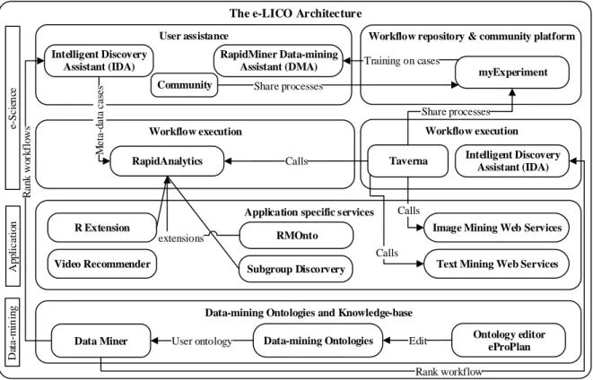
2.4.1.8 e-LICO . . . 28
2.4.1.9 Auto-WEKA . . . 30
2.4.2 Regression and Classification . . . 30
2.4.3 Clustering . . . 33
2.4.4 Discussion and Summary . . . 34
2.5 Adaptive Mechanisms . . . 37
2.5.1 Recurring Concept Extraction . . . 37
2.5.2 Periodic Algorithm Selection . . . 38
2.5.3 Meta-level Representation of Non-stationary Problems . . . 41
2.5.4 Discussion and Summary . . . 42
2.6 Hyper-parameter Optimization . . . 44
2.6.1 Transfer Learning of Deep Models . . . 45
2.6.2 Meta-Reinforcement Learning . . . 47
2.7 Research Challenges . . . 49
2.8 Problem Formulation . . . 53
3 Cross-domain Meta-learning for Time-series Forecasting 55 3.1 Methodology . . . 56
3.2 Experimentation Environment . . . 57
3.2.1 Examples of Datasets . . . 57
3.2.2 Base-level Forecasting Methods . . . 57
3.2.2.1 Simple time-series Algorithms . . . 58
3.2.2.2 Complex time-series Algorithms . . . 58
3.2.3 Meta-feature Generation . . . 59
3.2.3.1 Descriptive Statistics . . . 59
3.2.3.2 Frequency Domain and Autocorrelations . . . 60
3.2.4 Meta-knowledge Preparation . . . 61 3.2.5 Meta-learning . . . 62 3.2.6 Cluster Analysis . . . 64 3.3 Results . . . 64 3.4 Analysis . . . 65 3.5 Summary . . . 68
4 Towards Meta-learning of Deep Architectures for Efficient Domain Adap-tation 71 4.1 Methodology . . . 71
4.2 Experimentation Environment . . . 73
4.2.1 Datasets . . . 74
4.2.2 Pre-trained Image Classification Networks . . . 74
4.2.2.1 Inception-ResNet-v2 . . . 76
4.2.2.2 VGG-19 . . . 76
4.2.2.3 Inception-v3 . . . 76
4.2.3 Transfer Learning . . . 76
CONTENTS
4.4 Summary . . . 80
5 A Meta-Reinforcement Learning Approach to Optimize Parameters and Hyper-parameters Simultaneously 83 5.1 Methodology . . . 84
5.1.1 Meta-learner . . . 85
5.1.2 Base-learner . . . 86
5.1.2.1 Residual Block with Stochastic Depth . . . 87
5.2 Formulation . . . 87
5.3 Experimentation Environment . . . 90
5.3.1 Datasets . . . 90
5.4 Results and Analysis . . . 90
5.5 Summary . . . 94
6 Conclusions and Future Work 95 6.1 Research Challenges . . . 96
6.2 Main Findings and Contributions . . . 97
6.3 Future Research . . . 97
A Definitions 99
B Meta-features 105
C Summary of Literature Review 109
List of Tables
1 Terminologies . . . xv
2.1 Real-world datasets used in various studies . . . 6
2.2 List of publicly available Data Repositories . . . 8
2.3 Base-level learning strategies used in different studies . . . 21
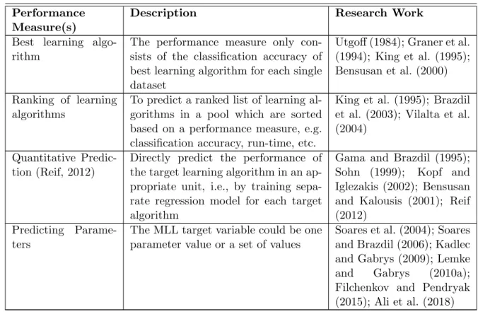
2.4 Different Performance Measures that are used in various literatures . . . 23
2.5 Existing Meta-learning Systems . . . 26
2.6 Meta-level learning strategy used in various studies . . . 35
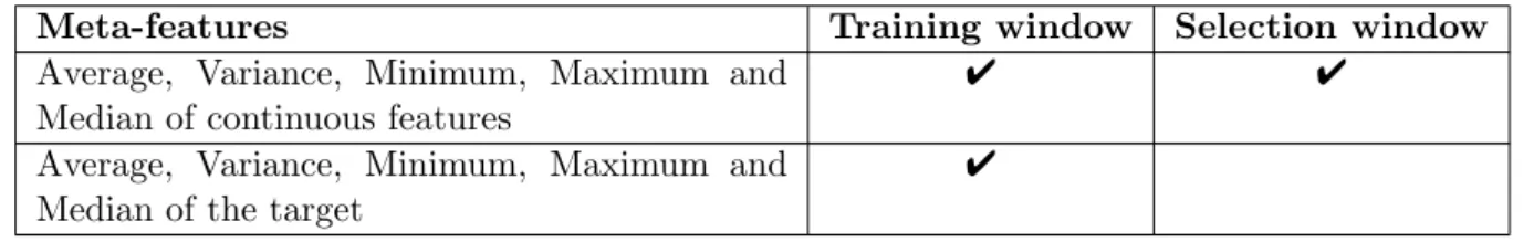
2.7 Meta-features used in MetaStream to characterize the data . . . 41
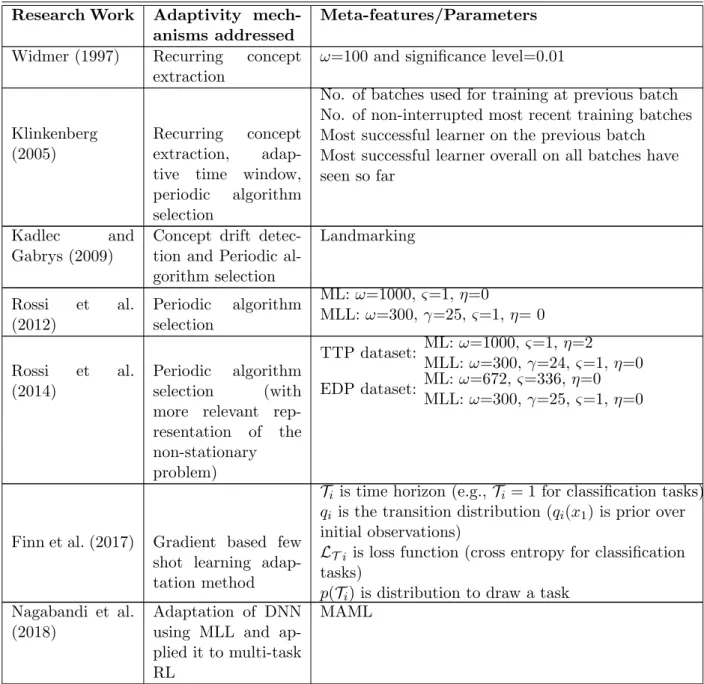
2.8 Adaptive mechanisms used in previous studies . . . 44
2.9 Hyper-parameter search techniques used in previous studies . . . 49
3.1 NN3, NN5 and NN-GC1 datasets which are used to build Meta-modelling and its evaluation . . . 58
3.2 Methods and their configurations that are used to compute performance mea-sures . . . 59
3.3 Symmetric Mean Absolute Percentage Error (SMAPE) and Standard Devia-tion (StdDev) of Base-level forecasting methods . . . 59
3.4 List of Meta-features (MFs) and their descriptions . . . 60
3.5 MFs Importance . . . 61
3.6 Proportion Raw and balanced classes . . . 62
3.7 SMAPE (and Accuracy) of various Meta-learners . . . 64
3.8 SMAPE (and StdDev) of NN-GC1 series . . . 65
3.9 SMAPE (and StdDev) of NN-GC1 series . . . 66
4.1 Open-source image repositories . . . 74
4.2 Benchmarking of various pre-trained image classification models . . . 74
4.3 Hyper-parameters that are used for transfer learning . . . 77
4.4 Transfer learning accuracies of various datasets, classification architectures, and their layers . . . 77
4.5 The state-of-the-art accuracy (training of the network from scratch) versus best possible accuracy from this work . . . 80
4.6 The similarity and average entropy of different datasets . . . 80
5.1 Hyper-parameter search space and parameters covering behaviour of the net-work that is used as states t+1 . . . 86
xii LIST OF TABLES
5.3 Comparison with different architecture search approaches on Cifar-10 dataset 91
5.4 Accuracy of various datasets including optimal parameters and episodes
List of Figures
2.1 Scope of existing research review . . . 5
2.2 Phase-wise collection of Examples of Datasets . . . 13
2.3 The LOF caption . . . 18
2.4 Combining Significant Meta-features from various approaches . . . 20
2.5 e-LICO project architecture . . . 29
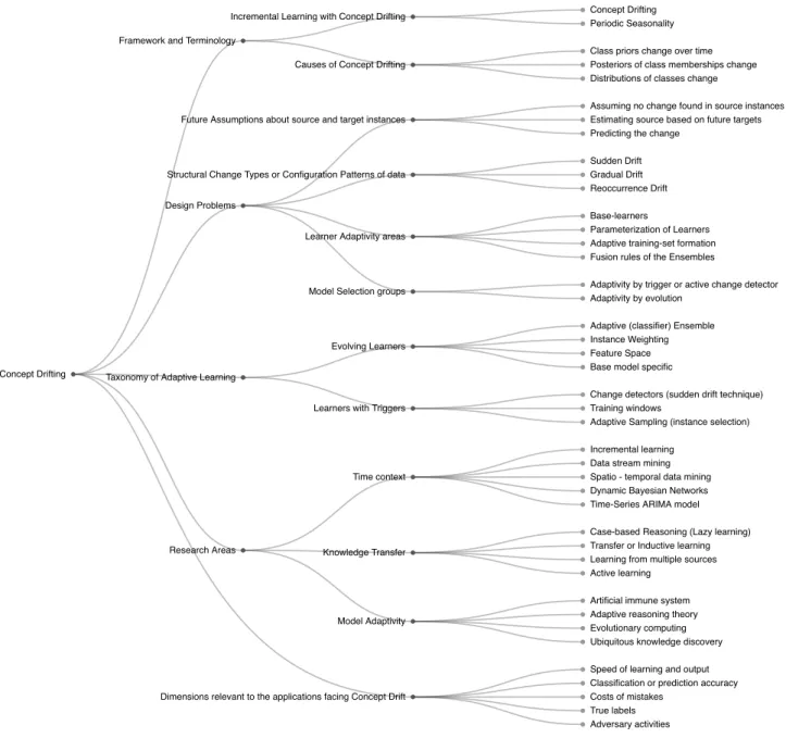
2.6 Learning under Concept Drifting (Zliobaite, 2010) . . . 40
2.7 A holistic view of Automatic Machine Learning areas and systems . . . 46
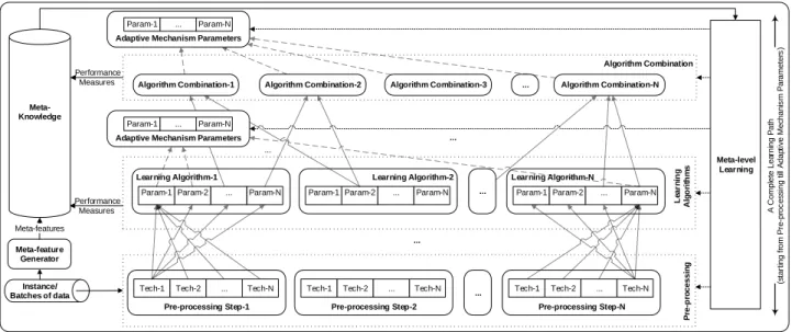
2.8 Learning Path Recommendation . . . 50
3.1 Methodology of Cross-domain Meta-level Learning (MLL) . . . 56
3.2 Histogram showing number of times a particular base and Meta-learner per-forms best for NN3, NN5 and combined NN3+NN5 data . . . 63
3.3 Histogram showing number of times a particular method performs best for NN-GC1 . . . 67
3.4 NN3 clustered together with NGGC-C dataset where the cluster cut over is at k = 20 . . . 68
4.1 Schematic diagram of transfer learning . . . 72
4.2 Transfer learning scenarios . . . 73
4.3 Schematic view of Inception-v3, Inception-ResNet-v2 and VGG-19 networks where the blue colour is representing a re-trainable layer/block. . . 75
4.4 Transfer learning accuracies of pre-trained networks; (a) Inception, (b) Inception-ResNet and (c) VGG-19 on ImageNet . . . 78
4.5 Inception-v3 blocks vs dataset size/class ration trend . . . 79
4.6 Datasets similarity with ImageNet for; (a) Inception-v3, (b) Inception-ResNet-v2 and (c) VGG-19 architectures. The similarity is normalized so that it can fit in between the scale of 1-10 with entropy. It is multiplied by 10. . . 81
5.1 A typical setting of Meta-Reinforcement Learning (Meta-RL) framework where agent contains a policy gradient and network sits in the environment . . . . 85
5.2 A schematic view of base-learner with maximum depth 4 and current depth 3 88 5.3 Cifar-10 time taken versus network validation accuracy plot . . . 92
5.4 Statistics of different datasets including policy loss, reward and network ac-curacy . . . 93
Terminologies and Mathematical
Definitions
Table 1: Terminologies
Symbol Description
A Set of finite actions, a∈ A
D Input/class dataset
s Possible experiences of D
Tr Training experience of D at any given moment
DTr Domain-specific dataset
f Function/Predictive model
p Probability function
α Learning rate
L Loss function
Cross-validation error on training data
φ Classification errors
πtheta Set of base-level classifiers
θ Parameters of each classifier
Lmu Supervised learning
µ Set of chosen base-algorithms
p Momentum
φ Probability distribution function
ρ Correlation coefficient
ω Training window (adaptability)
ς Step size (adaptability)
τ Tune temperature (adaptability)
λ Set of hyper-parameters
R Reward function
S Set of finite states, s ∈ S
T State transition probability
γ Discount factor
Glossary of Terms
A
A2C Actor-Critics. 37
AL Average Linkage. 36
ARIMA Auto-regressive Integrated Moving Average. 22, 32, 34, 36, 58, 59, 61, 62, 65–67
ARR Adjusted Ratio of Ratios. 15, 22
Auto-ML Automatic Machine Learning. 1, 4, 28, 30, 44, 45, 50, 68, 83
Auto-WEKA Automatic model selection and hyper-parameter optimization in WEKA.
28, 30
Average Nodes Average Nodes Learner. 107
B
b Number of Binary Features. 105
BLL Base-level Learning. 4, 20, 21, 23, 30, 31, 38, 42, 43, 52, 65, 95 C
C4.5 C4.5 Decision Tree algorithm. 15, 21, 22, 35
C5.0 boost C5.0 Adaptive Boosting. 15, 20–22, 35, 107
C5.0 rules C5.0 Rule Induction. 21, 22, 35, 107
C5.0 tree C5.0 Decision Tree. 15, 21, 22, 35, 107
CANCOR Canonical Correlation. 105
CART Classification and Regression Trees. 21, 22, 41
CASH Combined Algorithm Selection and Hyper-parameter Optimization. 28, 30
CASTLE Causal Structure for Inductive Learning. 21
xviii Glossary of Terms
CL Complete Linkage. 36
CN2 CN2 Induction Algorithm. 21, 35
CNN Convolutional Neural Network. 45–48, 74, 80, 86, 87, 89, 98
CORR Mean Absolute Correlation Coefficient. 31, 36, 106
CoV Coefficient of Variation. 33
CV Cross-Validation. 21, 22, 31
D
DBS DB-Scan. 36
DCT Dataset Characterization Tool. 14–17, 19, 30, 34
DDPG Deep Deterministic Policy Gradients. 49
Decision Nodes Decision Nodes Learner. 35, 107
DiscFunc Number of Discriminant Functions. 106
DL Deep Learning. 12, 44, 45, 47, 95
DMA Data Mining Advisor. 25, 27, 29, 34
DNN Deep Neural Networks. 1, 4, 19, 20, 36, 37, 43–45, 47, 50, 69, 82, 83, 94, 95, 97
DP Dynamic Programming. 102
DSIT Descriptive, Statistical, and Information-Theoretic. 2, 13–19, 25–27, 30, 34–37, 40, 43
DT Decision Trees. 16, 17, 19, 32, 36, 37, 62, 64–66
DW Durbin-Watson statistic of regression residual. 106
E
e-LICO e-Laboratory for Interdisciplinary Collaborative Research. 28, 29, 34
ENAS Efficient Neural Architecture Search. 49, 84, 94, 97
e-NN Elite-Nearest Neighbour. 35, 107
EoD Examples of Datasets. 5, 11, 12, 19, 23, 28, 44, 65, 68, 69, 95, 96
ES Exponential Smoothing. 22, 36
Glossary of Terms
FC Fully-Connected. 76, 77, 86
FF Farthest First. 36
FFT Fast Fourier Transform. 60
FLD Fisher’s Linear Discriminant. 21
FRACT Relative proportion of largest Eigenvalue. 106
G
GPU Graphics Processing Unit. 47, 49, 73, 90, 91
H
HC Entropy of Classes. 106
HCX Joint Entropy of Classes. 106
HPO Hyper-parameter Optimization. 1, 4, 28, 30, 45, 47, 48, 50, 71, 80, 94, 95, 98 I
IBL Instance-based Learning. 21, 22, 35
ICA Independent Component Analysis. 17
ID3 Iterative Dichotomiser 3. 35
IDA Intelligent Discovery Assistant. 26–28, 34
ILSVRC ImageNet Large-Scale Visual Recognition Challenge. 47, 76
INDCART Inductive CART. 21, 35
K k Number of Classes. 105 KD Knowledge Discovery. 26 k-M k-Means. 36 k-NN k-Nearest Neighbour. 17, 19–22, 31, 32, 35, 36, 107 KURT Kurtosis. 105, 106 L
LazyDT Lazy Decision Trees. 35
xx Glossary of Terms
LSTM Long Short-term Memory. 85
Ltree Linear Discriminant Trees. 21, 22, 35, 107
LVQ Learning Vector Quantization. 35
M
M Mixture Models. 36
MA Moving Average. 22, 32, 57–59, 61, 64–67, 69
MAE Mean Absolute Error. 21–23
MAML Model-Agnostic Meta-Learning. 43, 44, 48
MARS Multivariate Adaptive Regression Splines. 22
MCMLPS Multi-component, Multi-level Predictive System. 4
MCX Average Mutual Information between Class and Nominal Features. 106
MDP Markov Decision Process. 47
MDS Multi-dimensional Scaling. 17
ME Meta-example. 35, 41, 51, 52
METAL Meta-learning Assistant. 6, 15, 25, 27, 30, 31
METALA Meta-learning Architecture. 25, 27
Meta-RL Meta-Reinforcement Learning. xiii, 4, 19, 44, 45, 48, 53, 83–85, 89, 97, 98
MF Meta-feature. xi, 1, 2, 5, 9–21, 23–27, 30–35, 38, 40–44, 51, 52, 56, 57, 59–62, 65, 66, 68, 69, 82, 95, 96
MK Meta-knowledge. 1, 5, 11, 12, 20, 23, 28, 30, 31, 33, 35, 37, 51–53, 55–57, 61, 62, 64, 65, 67, 71
ML Machine Learning. 1, 5, 9, 11, 12, 24, 28, 30, 32, 37, 44, 47, 50, 53, 83, 95, 97
MLL Meta-level Learning. xiii, 1–6, 9–12, 15–17, 19–21, 23–35, 37–45, 47, 49–53, 55–57,
61, 64–69, 71, 95–98
MLP Multi-layer Perceptron. 21, 22, 31, 33–36
MLR Multiple Linear Regression. 22
MLT Machine Learning Toolbox. 24, 27
MSE Mean Squared Error. 22, 31, 36
Glossary of Terms
N
N Total Instances. 105
n Number of Numeric features. 105
NAS Neural Architecture Search. 1, 45, 48–50, 84, 94, 95, 97, 98 NB Naive Bayes classifier. 15, 17, 21, 22, 35, 36, 107
NBT Naive Bayes/Decision-Tree. 35
NN Neural Network. 16, 22, 32, 36, 37, 59, 62, 64–67, 83
NoiseRaio Noise to Signal Ratio. 106
O
OC1 Oblique Classifier-1. 35
OneR One Rule Learner. 22, 35, 36
OpenML Open Machine Learning. 8, 9, 11, 12
OPGA On-policy Gradient Algorithms. 49
OPSRL Optimistic Posterior Sampling for Reinforcement Learning. 36
P
p Number of Features. 105
PaREn Pattern Recognition Engineering. 26, 28, 34
PCA Principal Component Analysis. 17, 19, 107
PDF Probability Density Function. 19
PEBLS Parallel Exemplar-Based Learning System. 35
PMF Probability Mass Function. 19, 20, 77, 79
PNAS Progressive Neural Architecture Search. 48, 49
PPO Proximal Policy Optimization. 49
PPR Projection Pursuit Regression. 22
Q
QPC Quality of Projected Clusters. 10, 17
xxii Glossary of Terms
R
r Number of Training instances. 105
Randomly Chosen Nodes Randomly Chosen Nodes Learner. 35, 107
RapidAnalytics open-source data-mining and predictive analysis solution. 29
RBF Radial-basis Function. 21, 22, 32, 35, 36, 62
ReLU Rectified Linear Units. 87
ResNet Residual Networks. 45, 86
RF Random Forests. 22, 36, 41, 61
Ripper Rule Learner. 15, 21, 22, 35, 107
RL Reinforcement Learning. 35–39, 43, 44, 47–49, 84, 94, 97, 98
RMSE Root Mean Squared Error. 22
RNN Recurrent Neural Network. 35, 46, 48, 85–87, 98
RW Random Walk. 22, 36
S
s Number of Nominal features. 105
S/D Ratio Homogeneity of Covariances. 105
SKEW Skewness. 105, 106
SL Single Linkage. 36
SMAPE Symmetric Mean Absolute Percentage Error. xi, 22, 33, 58, 59, 61, 62, 64–66,
106
SMART Smooth Multiple Additive Regression Technique. 21
SMBO Sequential Model-Based Optimization. 11, 28, 48
SMOTE Synthetic Minority Over-sampling TEchnique. 61
SNN Shared Nearest Neighbours. 36
SP Spectral Clustering. 36
SRCC Spearman’s Rank Correlation Coefficient. 22, 33
STABB Shift To A Better Bias. 24, 26
Glossary of Terms
StdDev Standard Deviation. xi, 58–60, 62, 64–66, 105–107
SVM Support Vector Machines. 17, 21, 22, 31–33, 36, 37, 41, 62, 64–66
SVR Support Vector Regression. 33, 34
T
t Number of Test instances. 105
TL Transfer Learning. 45, 47, 72, 76, 79, 80, 82
TPOT Tree-based Pipeline Optimization Tool. 28
TPU Tensor Processing Unit. 47
TRPO Trust Region Policy Optimization. 36, 49
TS Time-series. 4, 7, 8, 10, 20, 23, 31, 32, 34, 36, 55, 97, 106 U
UCI UCI Machine Learning Repository. 6, 7, 9–11, 15, 16, 28, 30
V
VBMS Variable-bias Management System. 13, 17, 24–26
VGG Visual Geometry Group. 76
W
Wlambda Wilks’lambda Distribution. 106
Worst Nodes Worst Nodes Learner. 107
X
Acknowledgements
First of all, I would like to thank my supervisors Prof. Bogdan Gabrys and Prof. Marcin Budka for their support, expert advice and invaluable feedback.
I would like to thank my colleagues and friends at Bournemouth University, specially to Manuel, Rashid, Amir and Bassma. I would also like to thank Bournemouth University staff for always being nice and helpful to me. Special thanks to Dr. Emili Balaguer, Dr. Damien Fay and Naomi Bailey.
Not forgetting wife Moona, for her constant support and understanding. Finally, I would like to express my gratitude to my parents for always encouraging me in the right direction in both personal and academic sense.
Chapter 1
Introduction
This chapter presents the Doctoral research, its area, and an overview of the contributions in the space of Meta-level Learning (MLL) and related areas. In order to provide a clear motivation, this chapter outlines the main challenges and goals which lead to the aims and objectives of this research. The details of the research challenges that lead to several research questions can be found in Chapter 2.7.
1.1
Background and Motivation
One of the major challenges in Machine Learning (ML) is to predict when one algorithm is more adequate than another to solve a learning problem (Prudencio et al., 2011). Tradition-ally, estimating the performance of algorithms involves an intensive trial-and-error process which often demands massive execution time and memory together with the support of ex-pert advice that is not always easy to acquire (Giraud-Carrier et al., 2004). MLL arises as a potential solution of this problem; it uses examples from various domains to produce an ML model, known as Meta-learner, which is responsible for associating the characteristics of a problem with the candidate algorithm giving optimized accuracy. The knowledge which is used by a Meta-learner is acquired from previously solved problems, where each problem is characterized by several features, known as Meta-features (MFs). MFs are combined with performance measures of ML algorithms, e.g., accuracy, to build a Meta-knowledge (MK) database. Learning at the base-level gathers experience within a specific problem, while MLL is concerned with accumulating experience over several learning problems (Giraud-Carrier, 2008).
Along with the MLL, Hyper-parameter Optimization (HPO) and Neural Architecture Search (NAS) are also key methods of Automatic Machine Learning (Auto-ML) (Yao et al., 2019). The goal of HPO is to find a set of hyper-parameters of an ML task which gives optimized performance. It becomes crucial for Deep Neural Networks (DNN) which, in turn, comes with a wide range of hyper-parameter choices. The success of the DNN is mostly credited to its ability to automatically extract the task-dependent features. This automation is now expanding towards architecture engineering to automatically design complex neural architectures, known as NAS.
MLL started to appear in the ML domain in 1980’s and was referred to by different, such as, dynamic bias selection (Rendell et al., 1987), algorithm recommender (Brazdil et
2 Aims and Objective
al., 2008), etc. Sometimes it is also confused with Ensemble methods (Duch et al., 2011). In order to get a comprehensive view of exactly what MLL is, a number of definitions have been proposed in various studies. Vilalta and Drissi (2002a) and Vanschoren (2011) define MLL as the understanding of how learning itself can become flexible according to the domain or task and how it tends to adapt its behaviour to perform better. Giraud-Carrier (2008) describes it as the understanding of the interaction between the mechanism of learning and concrete context in which that mechanism is applicable. Brazdil et al. (2008) view on MLL is that it is the study of methods that exploit Meta-knowledge to obtain efficient models and solutions by adapting the learning algorithms. To some extent, this definition is followed in this research as well.
Extracting MFs from a dataset plays a vital role in the MLL task. Several MF generation approaches are available to extract a variety of information from previously solved problems. The most commonly used approaches are descriptive (or simple), statistical, information theoretic, landmarking and model-based. The Descriptive, Statistical, and Information-Theoretic (DSIT) features are easy to extract from the dataset as compared to the other approaches. Most of them have been proposed in the same period and are often used together. These approaches are used to estimate the similarity of new data with the already analyzed datasets (Bensusan et al., 2000). Landmarking is the most recent approach that tries to relate the performance of candidate algorithms to the performance obtained by simpler and computationally more efficient learners (Pfahringer et al., 2000). The Model-based approach captures the characteristics of a problem from the structural shape and size of a model induced by the dataset (Peng et al., 2002). The decision tree models are mostly used in this approach, where properties are extracted from the tree, such as tree depth, shape, nodes per feature, etc. (Giraud-Carrier, 2008).
1.2
Aims and Objective
The research described in this thesis is closely related to INFER1, a European project which aimed to develop a software platform for predictive modelling applicable in different industries and to work in the adaptive soft sensors for real-time prediction, monitoring, and control in the process industry. The goal of this work is to do research on MLL strategies and approaches for effective reduction of the model search space. There are multiple areas of a predictive system where MLL can be used to efficiently recommend the most appropriate methods and techniques. Therefore, three areas of evolving predictive systems are identified where the applicability of MLL can be an effective and efficient approach. These areas are thoroughly discussed in Section 2.7.
1. A Learning Path Recommendation: An optimal learning path recommendation of the three interlinked components including; pre-processing steps, learning algorithms or their combination, and adaptivity mechanism parameters.
2. Recurring Concepts Extraction: In a non-stationary environment, the underlying dis-tribution of the incoming data keeps changing which in turn makes the most recent
1
INTRODUCTION Research Challenges
historical concept ineffective. A MLL system can extract the relevant concepts of the data to adapt the out-dated model.
3. Concept Drift Detection: In an adaptive mechanism retraining of model is usually trig-gered by a change detection process. MLL can help to automatically detect the concept drift and trigger the algorithm retraining process instantly.
1.3
Research Challenges
There has been a lot of interest in MLL approaches and significant progress has been made. There are still a number of outstanding issues some of which have been addressed in the earlier approaches. The main challenge of this work is research on MLL strategies and ap-proaches in context of; feature engineering for problem representation and learning strategy for algorithm recommendation. This problem leads to several research questions which are outlined as follows and discussed in detail in Section 2.7 along with the goals and objectives of this work.
1. Gathering examples of datasets to build a static Meta-knowledge database
2. Base-level Learning strategy to compute performance measures of Meta-examples 3. Feature generation and selection to represent a problem at Meta-level
4. Representation and storage of dynamically growing complex Meta-Knowledge database 5. Meta-level Learning strategy for algorithm and its hyper-parameter recommendation
From the above five research questions, 3 and 5 are addressed in this research.
1.4
Contributions
A thorough survey of the existing techniques has been performed aiming at giving a compre-hensive overview of the research directions pursued under the umbrella of MLL. It reconciles different approaches given in scientific literature while designing the MLL systems. There are three studies conducted in this thesis around model selection and hyper-parameter search using MLL. These studies are addressing one or more research challenges which are described in the above section. The original contributions of this work are:
1. Formulation of Model Selection and Hyper-parameters Optimization (MSHPO) along with three key areas of an evolving predictive system which leads to several research challenges (see Section 2.7).
2. An MLL approach for evaluating the hypothesis whether the additional cross-domain training data can be beneficial to achieve reasonably good performance on a new task in the context of an MLL system for time-series forecasting. Chapter 3 illustrates it in detail.
4 Organisation of the Thesis
3. An empirical study on the relationship between various characteristics describing the similarity of two tasks, and based on that, the amount of fine-tuning of a deep neural network required by a new task to achieve accuracy close to state-of-the-art. Further details can be found in Chapter 4.
4. An original approach for automatic hyper-parameter optimization of a Multi-component, Multi-level Predictive System (MCMLPS) which frames an efficient hyper-parameters selection and tuning as a reinforcement learning problem. Chapter 5 further elaborates this contribution.
5. A framework to automatically find a good set of hyper-parameters resulting in rea-sonably good accuracy, which at the same time is less computationally expensive than the existing approaches (see Chapter 5).
A significant part of the research presented in this thesis has appeared in the following publications:
1. Abbas Ali, Bogdan Gabrys and Marcin Budka. Cross-domain Meta-learning for
Time-series Forecasting. In Procedia Computer Science, 126(1), 9-18, Elsevier, 2018.
2. Abbas Ali, Marcin Budka and Bogdan Gabrys. Towards Meta-learning of Deep
Ar-chitectures for Efficient Domain Adaptation. In the 16th Pacific RIM International Conference on Artificial Intelligence (PRICAI), 2019.
3. Abbas Ali, Marcin Budka and Bogdan Gabrys. A Meta-Reinforcement Learning
Ap-proach to Optimize Parameters and Hyper-parameters Simultaneously. In the 16th
Pacific RIM International Conference on Artificial Intelligence (PRICAI), 2019.
1.5
Organisation of the Thesis
The next chapter covers the existing research in Auto-ML area, including some important components of an MLL system. Those components include sources of existing and automatic generation of datasets, Meta-feature generation, and selection using various approaches and Base-level Learning (BLL) algorithms performance measures; such as accuracy, execution time, etc. This is followed by sections discussing existing MLL systems in the context of their applicability to supervised and unsupervised algorithms. Furthermore, Chapter 2 illustrates the adaptive mechanism and HPO areas in detail. Based on the conclusions and recommen-dations explored from the literature review, the final sections describe the research challenges and problem formulation of this research. An experimental investigation of cross-domain MLL for Time-series (TS) Forecasting is elaborated in Chapter 3. Chapter 4 consists of an empirical study to identify how deep a pre-trained image classifier needs to be fine-tuned based on the characteristics of the new task. Chapter 5 discusses a Meta-Reinforcement Learning (Meta-RL) approach to optimize the parameters and hyper-parameters tuning of DNN simultaneously. This report is concluded in Chapter 6 with future directions for the next phase.
Chapter 2
Existing Research
Immense research has been concentrating on automating Machine Learning (ML) algorithm selection for the last three decades (Z¨oller and Huber, 2019). The focus of those studies is to explore various components of Meta-level Learning (MLL). The scope of the litera-ture review is confined to areas that are related to this research. The high-level overview of the components which are discussed in this chapter is shown in Figure 2.1. The first section presents ways of gathering real-world datasets and techniques to create synthetic datasets which are known as Examples of Datasets (EoD). These EoD are used to gen-erate Meta-features (MFs) and associated performance measures which are discussed in Sections 2.2 and 2.3 respectively. MF are combined with performance measures to build Meta-knowledge (MK) dataset which becomes the input of MLL. The last section illustrates adaptive mechanisms in the context of MLL which are an important aspect of this research.
2.1
Repository of Datasets
A repository of datasets representing various problems is one of the key components of
the MLL system. As Vanschoren (2011) states, ‘there is no lack of experiments being
done, but the datasets and information obtained often remain in the people’s heads and
labs’. This section explores the sources of real-world datasets that are used in the existing studies to build MK database. However, real-world datasets are usually hard to obtain but
Repository of Datasets Meta-knowledge Performance Measures Meta-features generation and Selection Meta-level
Learning Adaptive Mechanisms
6 Repository of Datasets
artificially generated datasets would be a possible solution to this problem. The following subsections sumerize the studies that are dealing with real-world data, those which elaborate the techniques to generate artificial datasets, and the published resources.
2.1.1
Real-world Datasets
The real-world datasets can be difficult to find and gather in the desired format. An effort has been made to extract useful sources of data from various studies. Table 2.1 presents datasets that are used in different researches for MLL purpose. Most of them are gathered from UCI Machine Learning Repository (UCI) (Bache and Lichman, 2013).
Table 2.1: Real-world datasets used in various studies
Research Work Datasets Sources Dataset Filters
King et al. (1995) 12 Satellite image, Hand-written digits,
Karhunen-Loeve digits, Vehicle silhou-ettes, Segment data, Credit risk, Bel-gian data, Shuttle control, Diabetes, Heart disease, German credit, Head in-jury (King, 1995)
Lindner and
Studer (1999)
80 UCI and DaimlerChrysler
-Sohn (1999) 19 Satellite image, Hand-written digits,
Karhunen-Loeve digits, Vehicle silhou-ettes, Segment data, Credit risk, Bel-gian data, Shuttle control, Diabetes, Heart disease, German credit, Head in-jury (King, 1995) and 7 other datasets used in StatLog project
Three datasets of
StatLog having cost information involved in misclassification
Berrer et al.
(2000)
58 Meta-learning Assistant (METAL)
project datasets
38 datasets with no missing values
Soares et al.
(2001)
45 UCI and DaimlerChrysler Dataset with more
than 1000 instances
Bernstein and
Provost (2001)
15 Balance Scale, Breast Cancer, Heart
dis-ease, Heart disease - compressed glyph visualization, German Credit Data, Di-abetes, Vehicle silhouettes, Horse colic, Ionosphere, Vowel, Sonar, Anneal, Aus-tralian credit data, Sick, Segment data (Bache and Lichman, 2013)
-Todorovski et al. (2002)
65 UCI and METAL project datasets 38 datasets with no
missing values
Brazdil et al.
(2003)
53 UCI and DaimlerChrysler Datasets with more
EXISTING RESEARCH Repository of Datasets
Bernstein et al. (2005)
23 Balance Scale, Heart disease, Heart
dis-ease, Heart disease - compressed glyph visualization, German Credit Data, Di-abetes, Vehicle silhouettes, Ionosphere, Vowel, Anneal, Australian credit data, Sick, Segment data, Robot Moves, DNA, Gene, Adult 10, Hypothyroid, Wave-form, Page blocks, Optical digits, In-surance, Letter, Adult (Bache and Lich-man, 2013)
-Peng et al. (2002) 47 UCI
-Kopf and Igleza-kis (2002)
78 UCI Dataset with less
than 1066 instances and the number of
attributes ranged from 4 to 69 Prudencio and Ludermir (2004) I: 99 Time-series (TS) and II: 645
I: Time-series Data Library1 and II: M3
competition2
I: Stationary data
and II: Yearly data
Prudencio and
Ludermir (2008)
50 WEKA project3 On average datasets
contain 4,392
in-stances and 14
features
Wang et al.
(2009)
46 and 5 Time Series Data-mining Archive4 and
Time Series Data Library5
Kadlec and
Gabrys (2009)
3 Thermal oxidiser, Industry drier, and
Catalyst activation datasets of process industry On-line prediction datasets Lemke and Gabrys (2010a) 2 con-sisting of 111 TS
NN36 - Monthly business with 52-126
observations and NN56- daily cash
ma-chine withdrawals with 735 observations in each series
NN5 including some missing values
Abdelmessih et
al. (2010)
90 UCI Datasets with more
than 100 instances
Duch et al. (2011) 5 and 2 Leukemia, Heart, Wisconsin, Spam,
and Ionosphere are real-world datasets gathered from UCI and two synthetic datasets parity and monks
1
http://datamarket.com/data/list/?q=provider:tsdl
2http://forecasters.org/resources/time-series-data/m3-competition
3Machine Learning Group at University of Waikatohttp://www.cs.waikato.ac.nz/ml/weka 4
http://www.cs.ucr.edu/~eamonn/time_series_data
5http://datamarket.com/data/list/?q=provider:tsdl 6Neural Network forecasting competition
8 Repository of Datasets
Rossi et al. (2014) 2 Travel Time Prediction (TTP)
con-sists of 24,975 instances and Electric-ity Demand Prediction (EDP) consists of 27,888 instances
Feurer et al.
(2014)
57 Open Machine Learning (OpenML)
datasets
-Kuhn et al. (2018) 38 OpenML datasets The datasets have no
missing values and a binary outcome
Ali et al. (2018) 2
con-sisting of 111 TS
NN3 and NN5 NN5 including some
missing values
Warden (2011) handbook and Stanford and Iriondo (2018) cover the most useful sources of publicly available datasets. A lot of new sources of free and public data that have emerged over the last few years are discussed. Apart from discussing data-sources, methods to get datasets in bulk from those sources are also discussed in detail. Table 2.2 presents most of the sources from the author’s book.
Table 2.2: List of publicly available Data Repositories
Source Description Datasets Domain
AnalcatData Datasets that are used by Jeffrey S.
Si-monoff in his book Analyzing Categorical
Data, published in July 2003
83 Cross-domain
Amazon Web Ser-vices
A centralized repository of public datasets Astronomy,
Bi-ology,
Chem-istry, Climate,
Economics,
Ge-ographic and
Mathematics
Bioassay data Virtual screening of bioassay
(ac-tive/inactive compounds) data by
Amanda Schierz
21 Life Sciences
Canada Open
Data
Canadian government and geospatial data Government &
Geospatial
Datacatalogs List of the most comprehensive open data
catalogs
data.gov.uk Data of UK central government
depart-ments, other public sector bodies and local authorities
9616 Government and
Public Sector data.london.gov.uk Data of UK central government
depart-ments, other public sector bodies and local authorities
563 Government and
Public sector Data.gov/
Educa-tion
EXISTING RESEARCH Repository of Datasets
ELENA Non-stationary streaming data of flight
ar-rival and departure details for all the com-mercial flights within the USA
13 fea-tures and 116 million in-stances Aviation
KDD Cup Annual Data Mining and Knowledge
Dis-covery competition datasets
Cross-domain National
Govern-ment Statistical
Web Sites
Open Data Census
US Census Bureau Assesses the state of open data around theworld GovernmentPublic sector and
OpenData from
Socrata
Freely available datasets 10,000 Business,
Educa-tion, Government, Social and Enter-tainment
Open Source
Sports
Many sports databases, including Base-ball, FootBase-ball, Basketball and Hockey
Entertainment
UCI A collection of databases, domain
theo-ries, and data generators that are used by the ML community for the empirical anal-ysis of learning algorithms
199 Physical Sciences,
Computer Science & Engineering, So-cial Sciences, Busi-ness and Game
Yahoo Sandbox
datasets
Language, graph, ratings, advertising and marketing, competition, computing sys-tems and image datasets
- Cross-domain
OpenML From 100 OpenML classification datasets,
38 datasets without missing values and with a binary outcome have been used
38 Cross-domain
2.1.2
Synthetic Datasets
MFs are used as predictors in an MLL system. Typically, many MFs are extracted from a dataset, thereby leading to a high-dimensional sparsely populated feature space which has always been a challenge for learning algorithms. Hence, to overcome this problem sufficient number of datasets is required which may not be possible only from real-world datasets as they can be hard to obtain. So, artificially generated datasets might help in solving this issue. Rendell and Cho (1990) work on systematic artificial data generation is considered as one of the initial efforts in this regard.
Bensusan and Giraud-Carrier (2000) used 320 artificially generated boolean datasets with 5 to 12 features in each one. These artificial datasets were benchmarked on 16 UCI and DaimlerChrysler real-world datasets. Similarly Pfahringer et al. (2000) generated 222 datasets, each containing 20 numeric and nominal features having 1K to 10K instances classified between 2 to 5 classes. Additionally, 18 real-world UCI problems were used to evaluate the proposed approach.
10 Repository of Datasets
Soares (2009) proposed a method to generate a large number of datasets by transforming the existing datasets, known asdatasetoids. An artificial dataset was generated against each symbolic attribute of a given dataset, obtained by switching the selected attribute with the target variable. This method was experimented on 64 datasets gathered from the UCI repository and it generated a total of 983 datasetoids. At the end, potential anomalies related to the artificial datasets are also discussed along with their proposed solutions are presented. Those anomalies could be: 1) the new target variable has missing values, 2) it is very skewed, and/or 3) the corresponding target variable might be completely unrelated to remaining features. One very simple solution proposed for these problems was to simply
discard the datasetoids which showed any of the above mentioned properties. This method
produced promising results, therefore enabling the generation of new datasets which could solve the scarce datasets problems.
Wang et al. (2009) used both synthetic and real-world TS from diverse domains for MLL based forecasting method selection study. The details of real-world datasets are given in Table 2.1 while remaining synthetic datasets were generated using statistical simulation to facilitate the detailed analysis of forecasting association with data characteristics. A total of 264 artificial datasets posses certain characteristics, i.e., perfect and strong trend, perfect seasonality, noise. The data is transformed into samples of 1000 instances for each original TS while it is unchanged for the number of data-points smaller than 1000.
Soares et al. (2009) generated 160 artificial datasets to obtain a wide representative range of cluster structures. There were two methods used to generate datasets; 1) a standard cluster model using Gaussian multi-variate normal distributions, and 2) Ellipsoid cluster generator. There were three parameters selected for both techniques including i) the number of clusters which were the same for both cases (2, 4, 8, 16), ii) dimensions (2, 20 for Gaussian, and 50, 100 for Ellipsoid), and iii) the size of each cluster for both techniques were the same (uniformity in [10, 100] for 2 and 4 clusters case and [5, 50] for 8 and 16 clusters case). For each of the 8 combinations of cluster number and dimension, 10 different instances were generated, giving 80 datasets in each method.
Duch et al. (2011) used two artificially generated datasets out of a total of seven whereas the remaining five are real-world problems. One artificially generated dataset has binary features, named as Parity, whereas the other one with nominal features is known asMonks. These optimal support features are computed using Quality of Projected Clusters (QPC) projection (Grochowski et al., 2008).
Reif et al. (2012a) presents a novel data generator approach for numerical features and classification datasets that can be used as input dataset for MLL; i.e. an entirely different
approach from the Soares (2009). The proposed system was able to generate datasets
using genetic programming with customized parameters. Also in this setting MLL can be supported in two different ways: 1) the MFs space can be filled in a more controlled way and the discovered ”empty areas” can be populated rather than generating random datasets, and 2) thoroughly investigating MFs based on their descriptive power which can be useful for certain MLL problems and generating datasets with MFs allows more controlled experiments that might lead to the significant utilization of particular MFs. Since the dataset was generating multiple MFs therefore this task was treated as a multi-objective optimization problem. The proposed system was able to incorporate a variable set of arbitrary MFs. The
EXISTING RESEARCH Repository of Datasets
user was able to build a custom set of MFs simply by providing the functions that compute the MFs.
Feurer et al. (2014) obtained 57 datasets, from the OpenML project (Rijn et al., 2013), to study the impact of their MLL based initialization of Sequential Model-Based Optimization (SMBO) variants. Lemke and Gabrys (2010a) and Ali et al. (2018) have used 222 univariate time-series from two different sources, NN3 (Crone, 2006) and NN5 (Crone, 2008) competi-tions. Each data-source contains 111 series with monthly and daily occurrences respectively. Kuhn et al. (2018) chose a subset from the OpenML classification datasets. The authors used the datasets without missing values and with a binary class.
2.1.3
Datasets from Published Research
Another source of EoD are the published ML studies. As ML is one of the most active research areas since last few decades where several experimentations have been conducted. These experiments become a very useful way of gathering EoD representing various domains. Also, the additional factor that usually comes with most of the datasets used in existing researches is performance measures. It is used as target variable in the context of an MLL system. It is very time, memory and processor consuming task to compute performance measures against a massive amount of datasets and numerous configurations of learning algorithms.
Due to space limitation on publications, researches usually publish only final results with minimal details. However, in context of MLL, relying on this minimal information leads to several problems, for example, in most of the instances researches only report the best algorithm, usually report limited number and detail of experimentations, mostly skip detailed configurations of the algorithms, etc. Vanschoren et al. (2014) introduced a novel platform for ML research known as OpenML. ML researchers can share datasets, algorithms, their configurations, and experiment setups on this platform which other researchers can use to compare results. OpenML framework is one of the possible solutions for most of the mentioned concerns which resolves two key challenges of MLL systems; i) gathering a massive number of datasets from different domains, and ii) performances of datasets.
2.1.4
Discussion and Summary
An ML system relies on training dataset to build a model. Similarly, at Meta-level, the MK dataset is used as training-set of MLL, whereas this MK dataset is dependent on sufficient number of EoD from different domains. These EoD are used to generate MFs which act as predictors and performance measures of these EoD on various learning algorithms and are used as target variable in the MK dataset. However, gathering a sufficient number of real-world datasets is quite difficult. The real-world datasets which are used in various studies for experimentations are listed in Table 2.1. Most of the studies gathered datasets from UCI with different filtering options and the remaining few studies gathered datasets from different data-mining competitions. In most cases, the number of EoD that are used to build MK is very low. The MLL systems can perform as better as trial-and-error approach by providing a significant number of EoD representing various domains. Table 2.2 identifies a number of real-world datasets representing different domains.
12 Meta-features Generation and Selection
Some MLL researches resolved this problem by building their MK datasets using arti-ficially generated EoD. They have adopted two different approaches to generate synthetic datasets; 1) by transforming real-world datasets; and 2) by utilizing statistical and
ge-netic programming approaches. Bensusan and Giraud-Carrier (2000), Pfahringer et al.
(2000), Soares (2009) and Wang et al. (2009) proposed different feature transformation ap-proaches to generate different combinations of datasets from the limited number of real-world datasets. The statistical and genetic programming approaches are proposed by Soares et al. (2009) and Duch et al. (2011) for MLL systems. In some approaches, statistical functions with threshold (or cut-off) values are used to generate data while others used optimization techniques. Reif et al. (2012a) proposed an intelligent technique which does not generate random data, but fill the MFs in a more controlled way by discovering and populating the empty areas of real-world datasets.
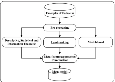
Combining all the proposed approaches iteratively seems to be a potential solution of dataset scarcity; i.e., initially gathering the existing available real-world problems, then transforming those datasets generating several others and finally applying various other techniques to generate artificial datasets independently (see Figure 2.2). Although this so-lution seems useful if the purpose is only gathering a massive number of EoD. But in the context of this research, the purpose of gathering these datasets is twofold; i) to generate MFs and ii) compute performance measures of these datasets against numerous learning algorithms and their configurations. Considering all three components of an MLL system, gathering datasets from published research seems more convincing where the performance measures are bundled with the EoD. However, there are a lot of challenges coupled with it for an MLL system which include reporting only the top performing learning algorithm, publishing limited information of experimentations, availability of datasets used in the re-search, detailed configurations of learning algorithm, etc. OpenML platform addresses most of these issues to some extent but it is in the preliminary stage which leads to several issues, for example, i) problem representation at Meta-level is covering very few domains, ii) most of the publications are using very few commonly used learning algorithms, etc.
Deep Learning (DL) is one of the recent advancement in ML which brought a paradigm shift in MLL (Minar and Naher, 2018). This shift has minimized the dependency of the MLL systems on a large repository of datasets (Hutter et al., 2018; Z¨oller and Huber, 2019; Yao et al., 2019).
2.2
Meta-features Generation and Selection
One of the primary applications of MLL is to recommend the best learning algorithm or to rank various algorithms against a problem that is further described by some new features, known as MFs. The role of such systems is to estimate the similarity between various problems which, in turn, requires the ability to estimate the similarity of new data with the already analysed datasets. There are three most commonly used MF generation approaches which allow to induce mapping between characteristics of a problem and learning algorithms. These approaches are discussed in the following sections.
EXISTING RESEARCH Meta-features Generation and Selection Dataset (DS) N Dataset (DS) 1 Real-world Datasets Transformed Datasets Transformations of real-world datasets Artificial Datasets Generating Artificial Datasets
Figure 2.2: Phase-wise collection of Examples of Datasets
2.2.1
Descriptive, Statistical and Information-Theoretic Approach
The Descriptive, Statistical, and Information-Theoretic (DSIT) approach is the simplest and most commonly used MF generation approach that extracts a number of DSIT measures of a problem. These measures are used to map the features of the problem to the algorithms (Giraud-Carrier, 2008). It is also supported by the empirical results that these simple characteristics, such as the size of the training set and input space play a vital role in differentiating suitability of various learning algorithms to solve such problems. The research works that have been performed using DSIT approach are reviewed below.
Rendell et al. (1987) proposed Variable-bias Management System (VBMS) that was one of the earliest efforts towards data characterization. Only two descriptive MFs, namely: the number of training instances and the number of features, were used to select the best among three symbolic learning algorithms. Later Rendell and Cho (1990) enhanced the existing system by adding useful MFs of complexity based on shape, size, and structure. Statistical and Logical learning (StatLog) project by King et al. (1995) further extended VBMS MFs by considering a larger number of dataset characteristics. A problem was described in the context of its descriptive and statistical properties. Several characteristics of a problem spanning from simple (descriptive) to more complex (statistical) ones were generated and later used by various studies. These characteristics were used to investigate why certain algorithms perform better on a particular problem as well as to produce a thorough empirical analysis of the learning algorithms.
Sohn (1999) initially used most of the datasets and MFs that were used in StatLog project which were later on enhanced with information-theoretic MFs. Furthermore, three new descriptive features were added by transforming the existing measures, for example, in the form of ratios. These MFs were used to rank several classification algorithms with considerably better performance as compared to the previous studies. The author has also
14 Meta-features Generation and Selection
claimed classification error and execution-time as important response variables to choose an appropriate classification algorithm for a problem.
In the same year Lindner and Studer (1999) proposed an extensive list of DSIT fea-tures of a problem under the name of Dataset Characterization Tool (DCT). The au-thors distinguished three categories of dataset characteristics; namely simple, statistical and information-theory based measures. The descriptive MFs have been used to extract general characteristics of the dataset, whereas statistical characteristics were mainly extracted from numeric attributes, while information-theoretic based measures from nominal attributes. As in StatLog, rules were generated to choose an algorithm for a given task. Having this in mind authors were motivated to propose Case-based Reasoning (CBR) approach to select the most suitable algorithm against a problem.
Reif et al. (2012b) presented a novel approach of generating informative MFs by simply averaging over all attributes of the source datasets. They proposed a two-fold approach; in the first fold MFs generate the DSIT features of the datasets using the traditional approach. The second fold describes differences over datasets that are not accessible using the typically used mean of Meta-measures that have been computed in the first fold. This approach preserves more information about such MFs while producing a feature vector with a fixed size. An additional level of features are extracted to automatically select the most useful features out of the available ones.
MFs that are used in the above studies are shown in Figure 2.3.
2.2.2
Landmarking Approach
Another technique of MF generation is Landmarking which characterizes a dataset using the performance of a set of simple learners. Its main goal is to identify areas in the input space where each of the simple learners can be regarded as an expert (Vilalta and Drissi, 2002a).
The basic idea behind landmarking is outlined as the performance of a learning algorithm on a task and discovering information about its nature. In this approach, the performance of a Base-learner on a problem reveals information about the nature of the problem. A landmark learner or landmarker is defined as the learning mechanism whose performance is used to describe a problem (Bensusan and Giraud-Carrier, 2000). Landmarkers posses a key property that their execution time is always shorter than the Base-learner’s time, otherwise, this approach would bring no benefit. Further, in this section, various studies dealing with Landmarking approach are discussed in detail.
One of the earliest studies on Landmarking was conducted by Bensusan and Giraud-Carrier (2000). This approach is claimed to be simpler, more intuitive and effective than the DSIT measures. A set of 7 landmarkers were trained on 10 different sets of equal size. Each dataset was then described by a vector of MFs (see Landmarkers branch of Figure 2.3), which are the error rates of the 7 landmarkers, and labelled by the target learners (see Landmarking section of Appendix B) which produce the highest accuracy. Several experimentations have been performed to compare the landmarking approach with DSIT. In the first experiment Landmarking was compared with 6 information-theoretic DCT features of Lindner and Studer (1999) (see information-theoretic MFs section of Figure 2.3).
EXISTING RESEARCH Meta-features Generation and Selection
In most of the cases of this experiment landmarking simply outperformed DSIT approach. In another experiment, the ability of landmarking to describe a problem and discriminate between two areas of expertise are highlighted. In most of the cases C5.0 Adaptive Boosting (C5.0 boost) (Quinlan, 1998) landmarker performed best. The last experiment benchmarked 16 real-world datasets from UCI (Bache and Lichman, 2013) and DaimlerChrysler where again landmarking approach has produced the overall best performance.
Pfahringer et al. (2000) also presented Landmarking while comparing it with the DSIT MF generation approach - DCT. They performed three types of experiments, namely 1) Artificial rule list and sets; 2) Selecting learning models, and 3) Comparing landmarking with information-theoretic approach. These experiments were almost the same as performed by Bensusan and Giraud-Carrier (2000), and the target learners (see Landmarking section of Appendix B) were the same as used in METAL project. In the first experiment, the set of landmarkers consisted of a Linear Discriminant Analysis (LDA), Naive Bayes classifier (NB), and C5.0 Decision Tree (C5.0 tree) learner. While base-learners performance relative to each other was predicted using C5.0 boost, LDA, and Rule Learner (Ripper). In addition to three landmarkers, 5 descriptive MFs (shown in descriptive approach of Figure 2.3) have also been extracted from 216 datasets. The Ripper was found to be the top performer in this experimentation. For selecting the best learning model experiment, the authors tried to investigate the capability of landmarking in deciding whether a learner involving multiple learning algorithms performs better than the other candidate algorithms. Here only C4.5 Decision Tree algorithm (C4.5) was used as Meta-learner trained with 222 artificial boolean datasets and tested with 18 UCI problems (Bache and Lichman, 2013). Even though the Landmarking accuracy was higher but it does not reflect on the overall performance of a system whose end goal is to accurately select a learning model. In the last experiment, the landmarking approach has been compared with the DSIT and also the combination of both approaches. 320 artificially generated binary datasets were produced where the combined approach performed best for all 10 Meta-learners followed by Landmarking with a significant difference as compared to DCT measure.
Soares et al. (2001) sample-based landmarkers were estimates of the performance of algorithms on a small sample of the data that had been used as predictors of the perfor-mance of those algorithms on the entire dataset. Additionally, relative landmarker addressed the inability of earlier landmarker to assess the relative performance of algorithms. This sampling-based relative landmarking approach was later compared with the DSIT DCT MFs (Lindner and Studer, 1999) as done by most of the landmarking studies. The ten algo-rithms, mentioned in Appendix B are used on 45 datasets, with more than 1000 instances, mostly gathered from UCI (Bache and Lichman, 2013) and DaimlerChrysler. These datasets
have been ranked by theNearest-Neighbour using Adjusted Ratio of Ratios (ARR) measure.
To observe the performance of the ranking method authors vary the value of k from 1 to
25. In comparison with other studies reported in the literature, a sample-based relative landmarking approach has shown improvements in algorithm ranking as compared with the traditional DCT measures.
Kopf and Iglezakis (2002) proposed a new approach of task description for model selec-tion in context of MLL. It evaluates the performance for assessing the quality standards for case-bases when used for supervised MLL. The case-base properties were used to assess the
16 Meta-features Generation and Selection
quality of given case-bases in terms of measures such as redundancy. A brief overview of necessary requirements for the implementation of the case-based properties has also been provided in their study. A comprehensive experimentation was performed to compare vari-ants of DCT DSIT approach, landmarking and their combinations. MFs were constructed for the experiments from UCI datasets (see Table 2.1) which contained up to 25% missing values. Error rates for ten different classification algorithms from the METAL project were determined for different subsets of data characteristics mentioned in Appendix B and re-stricted to three Base-learners that are shown in Figure 2.3. The empirical results show the proposed approach in combination with DSIT, and landmarking approaches as a promising one.
Abdelmessih et al. (2010) presented an overview of the RapidMiner’s Landmarking op-erator and its evaluation. This landmarking opop-erator was developed in an open-source data-mining tool RapidMiner. As mentioned repeatedly in the above studies, landmarkers selection is a critical process and the criteria to select an optimal landmarker consists of three characteristics: 1) a landmarker has to be simple, 2) it require minimum execution (processing) time and 3) it has to be simpler than the target learner(s). Following these con-ditions, RapidMiner provided the landmarkers shown in Figure 2.3 and target algorithms, for which the accuracy was predicted (see landmarking section of Appendix B). For the evaluation of these landmarkers, 90 datasets from the UCI (Bache and Lichman, 2013) and other sources are gathered with at least 100 samples in each. By following the existing studies, the landmarking operator has been compared with the DSIT MFs of StatLog (King
et al., 1995) and DCT (Lindner and Studer, 1999), where Landmarking has shown5.1-8.3%
overall boost in all cases.
2.2.3
Model-based Approach
Model-based MF generation is another effort towards task characterization in MLL domain. In this approach the dataset is represented in a data structure that can incorporate the complexity and performance of the induced hypothesis. Later the representation can serve as a basis to explain the reasons behind the performance of the learning algorithm Giraud-Carrier (2008). Several research works utilizing the Model-based approach are discussed as follows.
Bensusan et al. (2000) study was an initial effort towards the model-based approach. The authors proposed to capture the information directly from the induced decision trees for characterizing the learning complexity. Figure 2.3 lists the 10 descriptors computed from induced decision trees. Using these MFs, a task representation and algorithm to store and compare two different tree structures has been explained in detail with examples. Authors also elaborated the motivation of using the induced decision trees directly rather than the predefined properties used in decision tree based MFs that, in turn, made explicit properties implicit in the tree structure. Finally, higher-order MLL approach has been generalized by proposing data structures to characterize other algorithms. Tree-like structure was used for Decision Trees (DT) in this work, sets have been proposed for rule sets and graphs for Neural Networks (NNs).
EXISTING RESEARCH Meta-features Generation and Selection
Peng et al. (2002) effort was towards improving the dataset characterization by capturing structural shape and size of the decision tree induced from the dataset. For that purpose 15 features were proposed known as DecT, shown in Figure 2.3, which do not overlap with Bensusan et al. (2000). These measures have been used to rank 10 learning algorithms in various experiments. In the first experiment DCT (Lindner and Studer, 1999) DSIT MFs and 5 landmarkers (Worst Nodes Learner, Average Nodes Learner, NB, and LDA) were compared with DecT. The results proved the performance enhancement of the proposed approach. In another experiment, DecT measures have been compared with the same DCT measures and landmarkers to rank the learning algorithms based on accuracy and time where again DecT performed better. The last experiment was performed to select MFs by reducing the number of features to 25, 15 and 8 respectively. The k-Nearest Neighbour algorithm, with various values ofk between 1 to 40, was used to select k datasets for ranking the performance of learning algorithms. The results suggested that feature selection does not significantly influence the performance of either DecT or even DCT, furthermore, DecT outperformed other approaches.
The Neuro-cognitive inspired mechanism is proposed by Duch et al. (2011) to analyse learning based transformations that generate useful hidden features for MLL. The types of transformations include restricted random projections, optimization using projection pur-suit methods, similarity and general kernel-based features, conditionally defined features, and features derived from partial successes of various learning algorithms. The binary fea-tures were extracted from DT and rule-based algorithms where continuous feafea-tures were discovered by projection pursuit, linear Support Vector Machines (SVM) and simple pro-jections. NB provides posterior probabilities along these lines while k-Nearest Neighbour (k-NN) and kernel methods find similarity-based features. The proposed approach illustrates Multi-dimensional Scaling (MDS) mappings and Principal Component Analysis (PCA), In-dependent Component Analysis (ICA), QPC, SVM projections in the original, one- and two-dimensional space. Various real-world and synthetic datasets (details can be found in Table 2.1) were used for visualization and to analyse the kind of structures they create. The classification accuracies of the datasets are predicted using five classifiers including NB, k-NN, Separability Split Value Tree (SSV), Linear and Gaussian kernel SVM in the original, one- and two-dimensional spaces. The results show an significant improvement almost in all five algorithms as compared to the existing approach of the authors.
2.2.4
Discussion and Summary
There are three common MF generation approaches proposed in the reviewed publications for MLL: 1) DSIT, 2) Landmarking and 3) Model-based. The DSIT MFs approach was introduced at the early stage of MLL development where Rendell et al. (1987) proposed two descriptive features for VBMS. Later on Rendell and Cho (1990) added more descriptive features to the original list. The statistical MFs were introduced by King et al. (1995), and Sohn (1999) proposed information-theoretic features combined with some existing descrip-tives to represent a problem at Meta-level. Finally, Lindner and Studer (1999) proposed an extensive list of DSIT MFs, known as DCT. The DCT measures became a benchmarked approach to represent a problem using DSIT approach. These measures were later used in