Generalized Mixability via Entropic Duality
Mark D. Reid [email protected]
Australian National University & NICTA
Rafael M. Frongillo [email protected]
Harvard University
Robert C. Williamson [email protected]
Nishant Mehta [email protected]
Australian National University & NICTA
Abstract
Mixability is a property of a loss which characterizes when constant regret is possible in the game of prediction with expert advice. We show that a key property of mixability generalizes, and the expandlogoperations present in the usual theory are not as special as one might have thought. In doing so we introduce a more general notion ofΦ-mixability whereΦis a general entropy (i.e., any convex function on probabilities). We show how a property shared by the convex dual of any such entropy yields a natural algorithm (the minimizer of a regret bound) which, analogous to the classical Aggregating Algorithm, is guaranteed a constant regret when used withΦ-mixable losses. We characterize whichΦhave non-trivialΦ-mixable losses and relateΦ-mixability and its associated Aggregating Algorithm to potential-based methods, a Blackwell-like condition, mirror descent, and risk measures from finance. We also define a notion of “dominance” between different entropies in terms of bounds they guarantee and conjecture that classical mixability gives optimal bounds, for which we provide some supporting empirical evidence.
Keywords:online learning, prediction with expert advice, convex analysis, aggregating algorithm
1. Introduction
The combination or aggregation of predictions is central to machine learning. Traditional Bayesian updating can be viewed as a particular way of aggregating information that takes account of prior information. This is known to be special case of more general and decision theoretic “aggregating algorithms” (Vovk,2001) which take into account loss functions when evaulating predictions. As recent work by Gravin et al. (2014) shows, there are still a number of open questions about the optimal algorithms for the aggregation of predictions from a finite number of experts. In this paper, we attempt to address these by refining and generalizing the notion of “mixability” (Vovk,1990, 1998), which plays a central role in the theory of prediction with expert advice, characterizing the optimal learning rates in the asymptotic case of infinitely many experts.
We show there is an implicit design variable in mixability that to date has not been fully ex-ploited. The aggregating algorithm makes use of a divergence between the current distribution and a prior which serves as a regularizer. In particular the aggregating algorithm uses the KL-divergence. We consider the general setting of an arbitrary loss and an arbitrary regularizer (in the form of a Bregman divergence) and show that we recover the core technical result of traditional mixability: if a loss is mixable in our generalized sense then there is a generalized aggregating algorithm which
can be guaranteed to have constant regret. The generalized aggregating algorithm is developed by optimizing the bound that defines our new notion of mixability.
Our approach relies heavily on the titular dual representations of convex “generalized entropy” functions defined for distributions over a fixed number of experts. By doing so we gain new insight into why the original mixability argument works and a broader understanding of when constant re-gret guarantees are possible. In addition, we also make a number of interesting connections between mixability, mirror descent algorithms, and notions of risk from mathematical finance.
1.1. Mixability in Prediction With Expert Advice Games
A prediction with expert advice game is defined by its loss, a collection of experts that the player must compete against, and a fixed number of rounds. Each round the experts reveal their predictions to the player and then the player makes a prediction. An observation is then revealed to the experts and the player and all receive a penalty determined by the loss. The aim of the player is to keep its total loss close to that of the best expert once all the rounds have completed. The difference between the total loss of the player and the total loss of the best expert is called the regret and is typically the focus of the analysis of this style of game. In particular, we are interested in when the regret is
constant, that is, independent of the number of rounds played.
More formally, letXdenote a set of possibleobservationsand letAdenote a set ofactionsor
predictionsthe experts and player can perform. Aloss` : A → RX assigns the penalty` x(a)to
predictinga ∈ Awhenx ∈ X is observed. The finite set of experts is denoted1Θand the set of distributionsΘis denoted∆Θ. In each roundt= 1, . . . , T, each expertθ ∈Θmakes a prediction
at
θ ∈ A. These are revealed to the player who makes a prediction ˆat ∈ A. Once observation
xt ∈ X is revealed the experts receive loss`
xt(atθ)and the player receives loss`xt(ˆat). The aim of the player is to minimize its regretRegret(T) := LT −min
θLTθ where LT := PT t=1`xt(ˆat) andLT θ = PT
t=1`xt(atθ). We will say the game hasconstant regret if there exists a player who can always make predictions that guaranteeRegret(T)≤R`,Θfor allT and all expert predictions {at
θ}Tt=1whereR`,Θis a constant that may depend on`andΘ.
Vovk(1990,1998) showed that if the loss for a game satisfies a condition called mixability then a player making predictions using the aggregating algorithm (AA) will achieve constant regret. Definition 1 (Mixability and the Aggregating Algorithm) Givenη > 0, a loss`: A → RX is
η-mixableif, for all expert predictionsaθ ∈ A,θ ∈Θand all mixture distributionsµ ∈∆Θover
experts there exists a predictionaˆ∈ Asuch that for all outcomesx∈X, `x(ˆa)≤ −η−1log
X
θ∈Θ
exp (−η`x(aθ))µθ. (1)
Theaggregating algorithmstarts with a mixtureµ0 ∈∆
Θover experts. In roundt, experts predictatθ
and the player predicts theˆat∈ Aguaranteed by theη-mixability of`so that(1)holds forµ=µt−1
andaθ =atθ. Upon observingxt, the mixtureµt∈∆Θis set so thatµtθ ∝µtθ−1e−η`xt(atθ).
We note that our definition of mixability differs from the original in (Vovk,1998) and instead follows the presentation of mixability in (Cesa-Bianchi and Lugosi,2006). In particular, the orig-inal definition does not assume a fixed number of experts but instead quantifies (1) over allsimple 1. We use this notation to emphasize two points: 1) that expert predictions are parametric modelsp(x|θ)in the case of
distributions (i.e., with finite support) over actions, not experts. This departure from the original definition means that our definition of mixability depends on both the loss and the number of ex-perts rather than the loss alone. Crucially, this distinction allows us to formulate our generalization using generalized entropies and focuses attention on understanding bounds in the fixed, finite expert case.
As discussed in (Cesa-Bianchi and Lugosi,2006,§3.3), mixability can be seen as a weakening of exp-concavity that requires just enough of the loss to ensure constant regret.
Theorem 2 (Mixability implies constant regretVovk(1998)) If a loss ` is η-mixable then the aggregating algorithm will achieveRegret(T)≤η−1log|Θ|.
A natural question is whether there are other, similar algorithms which also enjoy constant regret guarantees or whether the specific definition in (1) is somehow special.
1.2. Contributions
The key contributions of this paper are as follows. We provide a new general definition (Defini-tion 4) of mixability and an induced generalized aggregating algorithm (Definition 7) and show (Theorem9) that prediction with expert advice using aΦ-mixable loss and the associated gener-alized aggregating algorithm is guaranteed to have constant regret. The proof illustrates that the particular form of (1) for the classical aggregating algorithm is not what guarantees constant regret, but rather it is a translation invariant property of the convex conjugate of an entropyΦdefined on a probability simplex that is the crucial property.
We characterize (Theorem6) for which entropiesΦthere existΦ-mixable losses via the Legen-dre property. We show thatΦ-mixability of a loss can be expressed directly in terms of the Bayes risk associated with the loss (Definition 13 and Theorem 15), reflecting the situation that holds for classical mixability (van Erven et al., 2012). As part of this analysis we show that multiclass proper losses are quasi-convex (Lemma 14) which, to the best of our knowledge appears to be a new result. We also show (Theorem 11) how entropic duals relate to the potential-based analysis ofCesa-Bianchi and Lugosi(2003).
1.3. Related Work
The starting point for mixability and the aggregating algorithm is the work ofVovk(1998,1990). The general setting of prediction with expert advice is summarized in (Cesa-Bianchi and Lugosi, 2006, Chapters 2 and 3). There one can find a range of results that study different aggregation schemes and different assumptions on the losses (exp-concave, mixable). Variants of the aggre-gating algorithm have been studied for classically mixable losses, with a trade-off between tight-ness of the bound (in a constant factor) and the computational complexity (Kivinen and Warmuth, 1999). Weakly mixable losses are a generalization of mixable losses. They have been studied by Kalnishkan and Vyugin(2008) who show that there exists a variant of the aggregating algorithm that achieves regretC√T for some constantC. Vovk(2001, in §2.2) makes the observation that his Aggregating Algorithm reduces to Bayesian mixtures in the case of the log loss game. See also the discussion byCesa-Bianchi and Lugosi(2006, page 330) relating certain aggregation schemes to Bayesian updating.
The general form of updating we propose is similar to that considered byKivinen and Warmuth (1997, 1999) who consider finding a vector w minimizing d(w, s) + ηL(yt, w·xt) where s is
some starting vector,(xt, yt)is the instance/label observation at roundtandLis a loss. The key
difference between their formulation and ours is that our loss term is (in their notation)w·L(yt, xt)–
i.e., the linear combination of the losses of thextatytand not the loss of their inner product. Online
methods of density estimation for exponential families are discussed byAzoury and Warmuth(2001, §3) where the authors compare the online and offline updates of the same sequence and make heavy use of the relationship between the KL divergence between members of an exponential family and an associated Bregman divergence between the parameters of those members. The analysis of mirror descent byBeck and Teboulle(2003) shows that it achieves constant regret when the entropic regularizer is used. However, there is no consideration regarding whether similar results extend to other entropies defined on the simplex.
The idea of the more general regularization and updates is hardly new and connections between entropic duality and more general potential-based methods (Cesa-Bianchi and Lugosi,2006,2003) are readily made by choosing the potential to be an entropic dual, as discussed in§3.2. Interestingly, such potentials are already well studied in the mathematical finance literature where they are called convex risk measures (F¨ollmer and Schied,2004), as well as in the literature on prediction markets where they are called cost functions (Abernethy et al.,2013). Thus, our work can be seen as extend-ing existextend-ing connections between online learnextend-ing and predication market mechanisms (Frongillo et al.,2012;Chen and Vaughan,2010), as discussed in§3.3.
The key novelty is our generalized notion of mixability, the name of which is justified by the key new technical result (Theorem9 — a constant regret bound assuming the general mixability condition achieved via a generalized algorithm that is exactly the mirror descent algorithm (i.e., SANP) of Beck and Teboulle(2003) for the Bregman divergence generated byΦ. Crucially, our result depends on some properties of the conjugates of functions defined over affine spaces (e.g., probabilities) that do not hold for potential functions more generally. By separating the convex geometry from the other special properties of classical entropy and mixability we hope to gain a deeper understanding of which losses admit fast rates of learning.
2. Generalized Mixability and Aggregation via Convex Duality
In this section we introduce our generalizations of mixability and the aggregating algorithm. One feature of our approach is the way the generalized aggregating algorithm falls out of the definition of generalized mixability as the minimizer of the mixability bound. Our approach relies on concepts and results from convex analysis. Terms not defined below can be found in a reference such as Hiriart-Urruty and Lemar´echal(2001).
2.1. Definitions and Notation
A function Φ : ∆Θ → Ris called an entropy(on ∆Θ) if it is proper (i.e., −∞ < Φ 6= +∞), convex2, and lower semi-continuous. Forη >0, we writeΦ
η := η−1Φ. In the following example
and elsewhere we use1to denote the vector1θ = 1for allθ∈Θand|Θ|−11∈∆Θto denote the uniform distribution overΘ. The distribution with unit mass onθ∈Θwill be denotedδθ.
Example 1 (Entropies) The(negative) Shannon entropy H(µ) := Pθµθlogµθ; the quadratic
entropy Q(µ) := Pθ(µθ − |Θ|−11)2; the Tsallis entropies Sα(µ) := α−1 Pθµαθ+1−1
for 2. While the information theoretic notion of Shannon entropy as a measure of uncertainty is concave, it is convenient
α∈(−1,0)∪(0,∞); and theR´enyi entropiesRα(µ) =α−1 logPθµαθ+1
, forα∈(−1,0). We note that both Tsallis and R´enyi entropies limit to Shannon entropyα →0, and that R´enyi entropy
is convex for the given range (cf.Maszczyk and Duch(2008);van Erven and Harremo¨es(2014)).
Lethµ, videnote a bilinear functional ordualitybetweenµ∈∆Θandv∈∆∗Θ, where∆Θand∆∗Θ form a dual pair3. TheBregman divergenceassociated with a suitably differentiable entropyΦon ∆Θis given by
DΦ(µ, µ0) = Φ(µ)−Φ(µ0)−
µ−µ0,∇Φ(µ0) (2) for allµ∈∆Θandµ0 ∈ relint(∆Θ), the relative interior of∆Θ. Given an entropyΦ : ∆Θ → R, we define its entropic dual to be Φ∗(v) := sup
µ∈∆Θhµ, vi −Φ(µ) where v ∈ ∆∗Θ. Note that one could also write the supremum over some larger space by settingΦ(µ) = +∞ forµ /∈ ∆Θ so that Φ∗ is just the usual convex dual (cf. Hiriart-Urruty and Lemar´echal (2001)). Thus, all of the standard results about convex duality also hold for entropic duals provided some care is taken with the domain of definition (Frongillo,2013). Importantly, we note that although the unrestricted convex dual ofHisv7→Pθexp(vθ−1)its entropic dual isH
∗(v) = logP
θexp(vθ).
For differentiable Φ, it is known (Hiriart-Urruty and Lemar´echal, 2001) that the supremum definingΦ∗is attained atµ=∇Φ∗(v). That is,
Φ∗(v) =h∇Φ∗(v), vi −Φ(∇Φ∗(v)). (3)
A similar result holds forΦ by applying this result toΦ∗ and usingΦ = (Φ∗)∗. We will make repeated use of the following easily established properties of affinely restricted convex conjugation, of which entropic duality (i.e., conjugation of convex functions on the simplex) is a special case. This is closely related to an observation by (Hiriart-Urruty and Lemar´echal,2001, Prop. E.1.3.2), however we include a statement of the general result and proof of this result in AppendixA for completeness.
Lemma 3 IfΦ is an entropy over∆Θ then 1) for allη > 0, Φη∗(v) = η−1Φ∗(ηv); and 2) the
entropic dualΦ∗istranslation invariant– i.e., for allv∈∆∗Θandα∈R,Φ∗(v+α1) = Φ∗(v) +α and hence for differentiableΦ∗,∇Φ∗(v+α1) =∇Φ∗(v).
The translation invariance of Φ∗ is central to our analysis. It is what ensures ourΦ-mixability inequality (4) “telescopes” when it is summed. The proof of the original mixability result (Theo-rem2) uses a similar telescoping argument that works due to the interaction oflogandexpterms in Definition1. Our results show that this telescoping property is not due to any special properties oflogandexp, but rather because of the translation invariance of the entropic dual of Shannon en-tropy,H. The remainder of our analysis generalizes that of the original work on mixability precisely because this property holds for the dual of any entropy.
Representation results from mathematical finance show that entropic duals are closely related to
convex monetary risk measures(F¨ollmer and Schied,2004), where translation invariance is called
cash invariance. In particular, the function ρ(v) = Φ∗(−v) for an entropy Φ (a.k.a. a penalty
function) is convex risk measure and is shown to be monotonic (i.e., v ≤ v0 pointwise implies ρ(v) ≥ρ(v0)). The risk measure corresponding to the Shannon entropy is known asentropic risk. 3. In the case of finiteΘthe duality is just the standard inner product. For infinite∆Θ, ∆∗Θ is a space of random
Furthermore, it can be shown that any measure of risk with these properties (convexity, mono-tonicity, and cash invariance) must be the convex conjugate of what we call an entropy (F¨ollmer and Schied,2004, Theorem 4.15). We note these results hold for general spaces of probability measures, which is why our presentation does not always assume a finite set of expertsΘ.
2.2. Φ-Mixability and the Generalized Aggregating Algorithm
For convenience, we will useA ∈ AΘto denote the collection of expert predictions andA
θ ∈ A
to denote the prediction of expertθ. Abusing notation slightly, we will write`(A)∈RX×Θfor the matrix of loss values[`x(Aθ)]x,θ, and `x(A) = [`x(Aθ)]θ ∈ RΘ for the vector of losses for each
expertθ on outcomex. In order to help distinguish between points, functions, distributions, etc.
associated with outcomes and those associated with experts we use Roman symbols (e.g.,x,A,p) for the former and Greek (e.g.,θ,Φ,µ) for the latter.
Definition 4 (Φ-mixability) LetΦbe an entropy on∆Θ. A loss`:A →RX isΦ-mixable if for
allA∈ AΘ, allµ∈∆
Θ, there exists anˆa∈ Asuch that for allx∈X
`x(ˆa)≤MixΦ`,x(A, µ) := inf µ0∈∆Θ µ0, `x(A) +DΦ(µ0, µ). (4)
The term on the right-hand side of (4) has some intuitive appeal. Sincehµ0, Ai=E
θ∼µ0[`x(Aθ)]
(i.e., the expected loss of an expert drawn at random according toµ0) we can view the optimization as
a trade off between finding a mixtureµ0that tracks the expert with the smallest loss upon observing
outcomexand keepingµ0 close toµ, as measured byDΦ. In the special case whenΦis Shannon
entropy,`is log loss, and expert predictionsAθ ∈∆Xare distributions overXsuch an optimization
is equivalent to Bayesian updating (Williams,1980;DeSantis et al.,1988).
To see thatΦ-mixability is indeed a generalization of Definition1, we make use of an alternative form for the right-hand side of the bound in theΦ-mixability definition that “hides” the infimum insideΦ∗. As shown in AppendixAthis is a straight-forward consequence of (3).
Lemma 5 For allA∈ Aandµ∈∆Θ, the mixability bound satisfies
MixΦ`,x(A, µ) = Φ∗(∇Φ(µ))−Φ∗(∇Φ(µ)−`x(A)). (5)
Hence, forΦ =η−1H,MixΦ
`,x(A, µ) =−η−1log
P
θexp(−η`x(Aθ))µθ, the bound in Definition1.
Later, we will useMixΦ`(A, µ)to denote the vector inRX with componentsMixΦ
`,x(A, µ), x∈X.
2.3. On the existence ofΦ-mixable losses
A natural question at this point is doΦ-mixable losses exist for entropies other than Shannon en-tropy? If so, which Φadmit Φ-mixable losses? The next theorem answers both these questions, showing that the existence of “non-trivial”Φ-mixable losses is intimately related to the behaviour of an entropy’s gradient at the simplex’s boundary. Specifically, we will say an entropyΦis
Legen-dre4if: a)Φis differentiable and strictly convex inrelint(∆
Θ); and b)k∇Φ(µ)k → ∞asµ→µb
4. We note that our definition is slightly different (but similar in spirit) to the standard definition of Legendre function (cf. (Rockafellar,1997)) since it requires a functionf be strictly convex on theinteriorofdom(f)and that the
for anyµb on the boundary of∆Θ. We call a loss`nontrivialif there existx∗, x0 anda∗, a0 such
that
a0 ∈arg min{`x∗(a) :`x0(a) = inf a∈A`x
0(a)}and inf a∈A`x
∗(a) =`x∗(a∗)< `x∗(a0). (6)
Intuitively, this means that there exist distinct actions which are optimal for different outcomes
x∗, x0. In particular, among all optimum actions forx0,a0 has the lowest loss onx∗. This rules out
constant losses –i.e.,`(a) =k∈RXfor alla∈ A– which are easily5seen to beΦ-mixable for any
Φ. For technical reasons we will further restrict our attention tocurvedlosses by which we mean those losses with strictly concave Bayes risks —i.e., the function L(p) := infa∈AEx∼p[`x(a)]is
strictly concave — though we conjecture that the following also holds for non-curved losses. Theorem 6 Non-trivial, curvedΦ-mixable losses exist if and only if the entropyΦis Legendre.
The proof is in AppendixA.4. We can apply this result to Example1and deduce that there are noQ-mixable losses. Also, since it is easy to show the derivatives∇Sαand∇Rα are unbounded
for α ∈ (−1,0), the entropies Sα and Rα are Legendre. Thus there exist Sα- andRα-mixable
losses whenα ∈ (−1,0). Due to this result we will henceforthrestrict our attention to Legendre entropies.
We now define a generalization of the Aggregating Algorithm of Definition 1that very natu-rally relates to our definition ofΦ-mixability: starting with some initial distribution over experts, the algorithm repeatedly incorporates information about the experts’ performances by finding the minimizerµ0 in (4).
Definition 7 (Generalized Aggregating Algorithm) The algorithm begins with a mixture
distri-butionµ0 ∈∆
Θover experts. On roundt, after receiving expert predictionsAt∈ AΘ, the general-ized aggregating algorithm(GAA) predicts anyˆa∈ Asuch that`x(ˆa)≤MixΦ`,x(At, µt−1)for allx
which is guaranteed to exist by theΦ-mixability of`. After observingxt∈X, the GAA updates the
mixtureµt−1∈∆ Θby setting µt:= arg min µ0∈∆Θ µ0, `xt(At)+DΦ(µ0, µt−1). (7) We now show that this updating process simply aggregates the per-expert losses`x(A)in the
dual space∆∗Θ with∇Φ(µ0) as the starting point. The GAA is therefore exactly theSubgradient
algorithm with nonlinear projections(SANP) for the Bregman divergenceDΦ(and a fixed step size of 1) which is known to be equivalent to mirror descent (Beck and Teboulle,2003) using updates based on∇Φ∗.
Lemma 8 The GAA updatesµtin(7)satisfy∇Φ(µt) =∇Φ(µt−1)−`
xt(At)for alltand so ∇Φ(µT) =∇Φ(µ0)−
T
X
t=1
`xt(At). (8)
The proof is given in Appendix A. Finally, to see that the above is indeed a generalization of the Aggregating Algorithm from Definition 1we need only apply Lemma8 and observe that for Φ =η−1H,∇Φ(µ) =η−1(log(µ) +1)and sologµt= logµt−1−η`
xt(At). Exponentiating this vector equality element-wise givesµt
θ∝µ t−1
θ exp(−η`xt(Atθ)).
3. Properties ofΦ-mixability
In this section we establish a number of key properties forΦ-mixability, the most important of these being thatΦ-mixability implies constant regret.
3.1. Φ-mixability Implies Constant Regret
Theorem 9 If`:A →RX isΦ-mixable then there is a family of strategies parameterized byµ∈
∆Θwhich, for any sequence of observations x1, . . . , xT ∈ X and sequence of expert predictions
A1, . . . , AT ∈ AΘ, plays a sequenceˆa1, . . . ,ˆaT ∈ Asuch that for allθ∈Θ T X t=1 `xt(ˆat)≤ T X t=1 `xt(Atθ) +DΦ(δθ, µ). (9) The proof is in AppendixA.1and is a straight-forward consequence of Lemma5and the trans-lation invariance ofΦ∗. The standard notion of mixability is recovered whenΦ = 1
ηHforη >0and
Hthe Shannon entropy on∆Θ. In this case, Theorem2is obtained as a corollary forµ=|Θ|−11, the uniform distribution overΘ. A compelling feature of our result is that it gives a natural inter-pretation of the constantDΦ(δθ, µ)in the regret bound: ifµis the initial guess as to which expert is
best before the game starts, the “price” that is paid by the player is exactly how far (as measured by
DΦ) the initial guess was from the distribution that places all its mass on the best expert. Kivinen and Warmuth(1999) give a similar interpretation to the regret bound for the special case ofΦbeing Shannon entropy in their Theorem 3.
The following example computes mixability bounds for the alternative entropies introduced in §2.1. They will be discussed again in§4.2below.
Example 2 Consider games withK=|Θ|experts and the uniform distributionµ=K−11∈∆ Θ.
For the (negative) Shannon entropy, the regret bound from Theorem9isDH(δθ, µ) = logK. For
the family of Tsallis entropies the regret bound given byDSα(δθ, K
−11) =α−1(1−K−α). For the
family of R´enyi entropies the regret bound becomesDRα(δθ, K
−11) = logK.
A second, easily established result concerns the mixability of scaled entropies. The proof follow from the observation that in (4) the only term in the definition ofMixΦη`,xinvolvingηisDΦη = 1ηDΦ. The quantification overA, µ,ˆaandxin the original definition has been translated into infima and
suprema.
Lemma 10 The functionM(η) := infA,µsupˆainfµ0,x MixΦη
`,x(A, µ)−`x(ˆa)is non-increasing.
This implies that there is a well-defined maximalη > 0for which a given loss`isΦη-mixable
sinceΦη-mixability is equivalent toM(η) ≥0. We call this maximalηtheΦ-mixability constant
for`and denote itη(`,Φ) := sup{η >0 :M(η)≥0}. This constant is central to the discussion in Section4.3below.
3.2. Relationship to Potential-Based Methods and the Blackwell Condition
Much of the analysis of online learning in Chapters 2, 3, and 11 of the book byCesa-Bianchi and Lugosi(2006) is based onpotential functions(Cesa-Bianchi and Lugosi,2003) and their associated
Bregman divergences. As shown below, when their potentials are entropic duals, we obtain some connections with their analysis. In particular, we will see that if a loss satisfiesΦ-mixability then theBlackwell conditionfor the potentialΨ = Φ∗is satisfied.
A loss function`satisfies theBlackwell condition(cf. (Cesa-Bianchi and Lugosi,2003)) for a convex potentialΨ :RX →Rif for allR ∈ RX andA∈ AΘthere exists someaˆ ∈ Asuch that supx∈Xh∇Ψ(R), rxi ≤ 0, whererx = `x(ˆa)1−`x(A). We now have the following result. The
proof is in SectionA.2.
Theorem 11 LetΦ : ∆X → Rbe an entropy with entropic dualΨ = Φ∗. If`is a loss function
that isΦ-mixable, then`satisfies the Blackwell condition for the convex potential functionΨ. 3.3. Φ-Mixability of Proper Losses and Their Bayes Risks
Entropies are known to be closely related to the Bayes risk of what are called proper losses or proper scoring rules (Dawid,2007;Gneiting and Raftery,2007). Here, the predictions are distributions over outcomes,i.e., points in∆X. To highlight this we will usep,pˆandPinstead ofa,ˆaandAto denote
actions. If a loss`: ∆X → RX is used to assign a penalty`x(ˆp)to a predictionpˆupon outcomex
it is said to beproperif its expected value underx∼pis minimized by predictingpˆ=p. That is,
for allp,pˆ∈∆X,
Ex∼p[`x(ˆp)] =hp, `(ˆp)i ≥ hp, `(p)i=:−F`(p),
where−F` is theBayes riskof`and is necessarily concave (van Erven et al.,2012), thus making
F` : ∆
X → Rconvex and thus an entropy. The correspondence also goes the other way: given
any convex functionF : ∆X →Rwe can construct a unique proper loss (Vernet et al.,2011). The
following representation can be traced back toSavage(1971) but is expressed here using convex duality.
Lemma 12 IfF : ∆X →Ris a differentiable entropy then the loss`F : ∆X →Rdefined by
`F(p) :=−∇F(p) +F∗(∇F(p))1=−∇F(p) + (h∇F(p), pi −F(p))1 (10)
is proper.
By way of example, it is straight-forward to show that the proper loss associated with the nega-tive Shannon entropyΦ =His the log loss, that is,`H(µ) :=−(logµ(θ))
θ∈Θ.
This connection between losses and entropies lets us define theΦ-mixability of a proper loss strictly in terms of its associated entropy. This is similar in spirit to the result byvan Erven et al. (2012) which shows that the original mixability (for Φ = H) can be expressed in terms of the
relative curvature of Shannon entropy and the loss’s Bayes risk. We use the following definition to explore the optimality of Shannon mixability in Section4.3below.
Definition 13 An entropyF : ∆X →RisΦ-mixableif
sup P,µ F∗ −MixΦ`F(P, µ) = sup P,µ F∗ Φ∗(∇Φ(µ)−`Fx(P)) x−Φ∗(∇Φ(µ))1≤0 (11)
where`F is as in Lemma12 and the supremum is over expert predictionsP ∈ ∆Θ
X and mixtures
Although this definition appears complicated due to the handling of vectors in RX andRΘ, it has a natural interpretation in terms of risk measures from mathematical finance (F¨ollmer and Schied,2004). Given some convex functionα : ∆X → R, its associated risk measure is its dual
ρ(v) := supp∈∆Xhp,−vi −α(p) = α∗(−v)wherevis apositionmeaningv
x is some monetary
value associated with outcomexoccurring. Due to its translation invariance, the quantityρ(v)is often interpreted as the amount of “cash” (i.e., outcome independent value) an agent would ask for to take on the uncertain positionv. Observe that the riskρF for whenα=F satisfiesρF ◦`F = 0
so that`F(p)is always aρF-risk free position. If we now interpretµ∗ =∇Φ(µ)as a position over
outcomes inΘandΦ∗as a risk forα = Φthe termΦ∗(µ∗−`F
x(P)) x−Φ
∗(µ∗)
1can be seen as the change inρΦ risk when shifting positionµ∗ toµ∗
−`F
x(P) for each possible outcome x.
Thus, the mixability condition in (11) can be viewed as a requirement that aρF-risk free change in
positions overΘalways beρΦ-risk free.
The following theorem shows that the entropic version ofΦ-mixability Definition13is equiv-alent to the loss version in Definition 4 in the case of proper losses. Its proof can be found in AppendixA.3and relies on Sion’s theorem and the facts that proper losses arequasi-convex (i.e., ∀λ∈[0,1],f(λx+ (1−λ)y)≤max{f(x), f(y)}). This latter fact appears to be new so we state it here as a separate lemma and prove it in AppendixA.
Lemma 14 If`: ∆X →RX is proper thenp07→ hp, `(p0)iis quasi-convex for allp∈∆X.
Theorem 15 If ` : ∆X → RX is proper and has Bayes risk−F thenF is an entropy and`is
Φ-mixable if and only ifF isΦ-mixable.
The entropic form of mixability in (11) shares some similarities with expressions for the clas-sical mixability constants given by Haussler et al. (1998) for binary outcome games and by van Erven et al.(2012) for general games. Our expression for the mixability is more general than the previous two being both for binary and non-binary outcomes and for general entropies. Computing the optimizing argument is also more efficient than in (van Erven et al.,2012) since, for non-binary outcomes, their approach requires inverting a Hessian matrix at each point in the optimization.
4. Conclusions and Open Questions
The main purpose of this work was to shed new light on mixability by casting it within the broader notion ofΦ-mixability. We showed that the constant regret bounds enjoyed by mixable losses are due to the translation invariance of entropic duals, and so are also enjoyed by anyΦ-mixable loss. Our definitions and results allow us to now ask precise questions about alternative entropies and the optimality of their associated aggregating algorithms.
4.1. Are All Entropies “Equivalent”?
Since Theorem6shows the existence of Φ-mixable losses for LegendreΦ, we can ask about the relationship between the sets of losses that are mixable for different choices ofΦ. For example, are there losses that areH-mixable but notSα-mixable, or vice-versa? We conjecture that essentially
all entropiesΦhave the sameΦ-mixable losses up to a scaling factor.
Conjecture 16 LetΦbe an entropy on∆Θand`be aΦ-mixable loss. IfΨis a Legendre entropy
Some intuition for this conjecture is derived from observing thatMixΨη`,x =η−1MixΨ
η`,xand that
asη → 0 the functionη`behaves like a constant loss and will therefore be mixable. This means that scaling upMixΨη`,xbyη−1should make it larger thanMixΦ
`,x. However, some subtlety arises in
ensuring that this dominance occurs uniformly. The discussion in AppendixBgives an example of two entropies where this scaling trick does not work.
4.2. Asymptotic Behaviour
There is a lower bound due toVovk(1998) for general losses`which shows that if one is allowed
to vary the number of roundsT and the number of expertsK = |Θ|, then no regret bound can be better than the optimal regret bound obtained by Shannon mixability. Specifically, for a fixed loss
`with optimal Shannon mixability constant η`, suppose that for someη0 > η` we have a regret
bound of the form(logK)/η0 as well as some strategyLfor the learner that supposedly satisfies
this regret bound. Vovk’s lower bound shows, for thisη0 andL, that there exists an instantiation
of the prediction with expert advice game withT large enough and K roughly exponential inT
(and both are still finite) for which the alleged regret bound will fail to hold at the end of the game with non-zero probability. The regime in which Vovk’s lower bound holds suggests that the best achievable regret with respect to the number of experts grows aslogK. Indeed, there is a lower
bound for general losses` that shows the regret of the best possible algorithm on games using`
must grow likeΩ(logK)(Haussler et al.,1998).
The above lower bound arguments apply when the number of experts is large (i.e., exponential in the number of rounds) or if we consider the dynamics of the regret bound as K grows. This leaves open the question of the best possible regret bound for moderate and possibly fixedKwhich
we formally state in the next section. This question serves as a strong motivation for the study of generalized mixability considered here. Note also that the above lower bounds are consistent with the fact that there cannot be non-trivial,Φ-mixable losses for non-LegendreΦ(e.g., the quadratic entropyQ) since the growth of the regret bound as a function ofK (cf. Example 2) is less than
logKand hence violates the above lower bounds. 4.3. Is There An “Optimal” Entropy?
Since we believe thatΦ-mixability for LegendreΦyield the same set of losses, we can ask whether, for a fixed loss`, someΦgive better regret bounds than others. These bounds depend jointly on the largestη such that`isΦη-mixable and the value ofDΦ(δθ, µ). We can define the optimal regret
bound one can achieve for a particular loss`using the generalized aggregating algorithm withΦη
for some η > 0. This allows us to compare entropies on particular losses, and we can say that an entropy dominates another if its optimal regret bound is better for all losses `. Recalling the
definition of the maximalΦ-mixability constant from Lemma10, we can determine a quantity of more direct interest: the best regret bound one can obtain using a scaled copy ofΦ. Recall that if`is
Φ-mixable, then the best regret bound one can achieve from the generalized aggregating algorithm isinfµsupθDΦ(δθ, µ). We can therefore define the best regret bound for`on a scaled version of
Φto beR`,Φ := η(`,Φ)−1infµsupθDΦ(δθ, µ)where η(`,Φ) denotes theΦ-mixability constant
for `. Then R`,Φ simply corresponds to the regret bound for the entropyΦη(`,Φ). Note a crucial
property ofR`,Φ, which will be very useful in comparing entropies: R`,Φ = R`,αΦ for allα > 0. (This follows from the observation thatη(`, αΦ) =η(`,Φ)/α.) That is,R`,Φis independent of the particular scaling we choose forΦ.
We can now use R`,Φ to define a scale-invariant relation over entropies. Define Φ ≥` Ψ if
R`,Φ ≤ R`,Ψ, andΦ ≥∗ ΨifΦ ≥` Ψfor all losses`. In the latter case we say ΦdominatesΨ.
By construction, if one entropy dominates another its regret bound is guaranteed to be tighter and therefore its aggregating algorithm will achieve better worst-case regret. As discussed above, one natural candidate for a universally dominant entropy is the Shannon entropy.
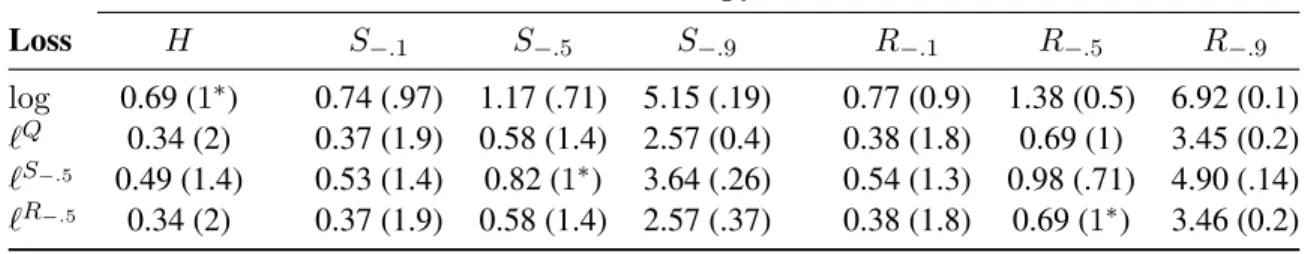
Conjecture 17 For all choices ofΘ, the negative Shannon entropy dominates all other entropies.
That is,H ≥∗ Φfor allΘand all convexΦon∆Θ.
Although we have not been able to prove this conjecture we were able to collect some positive evidence in the form of Table1in Appendix C. Here, we took the entropic form ofΦ-mixability from Definition13 and implemented it as an optimization problem and computedη(`F,Φ)forF
andΦequal to the entropies introduced in Example1for two expert games with two outcomes. The maximal η (and hence the optimal regret bounds) for each pair was found doing a binary search
for the zero-crossing of M(η) from Lemma 10 and then applying the bounds from Example 2. Although we expected the dominant entropy for each loss`F to be its “matching” entropy (i.e.,
Φ =F), the table shows the optimal regret bound for every loss was obtained in the column forH.
One interesting feature for these matching entropy and loss cases is that the optimalη(shown in
parentheses) is always equal to 1. We conjectured that`F would always beF-mixable with maximal
η = 1but found the counterexample described in AppendixB. However, we have not been able to rule out or prove the following weakenings of that conjecture. We observe that these cannot both be true due to the counterexample just described.
Conjecture 18 Suppose|X| = |Θ|so that∆Θ = ∆X andΦ : ∆Θ → Ran entropy. Then if its
proper loss`Φ : ∆
X →RX isΦ-mixable, the maximalηsuch that`Φisη−1Φ-mixable isη= 1.
Conjecture 19 If∆Θ= ∆X andΦis an entropy then`Φisη−1Φ-mixable for someη >0.
4.4. Future Work
Although Vovk’s original mixability result has the “asymptotic” converse described in §4.2, the above conjectures highlight our lack of understanding of when fast rates of learning are achievable in the non-asymptotic regime. As well as resolving these conjectures, we hope to use this work as a basis for developing necessary conditions for constant regret for a fixed number of experts.
Finally, there have been some recent papers (Steinhardt and Liang,2014;Orabona et al.,2015) which introduce extra time-varying updates (“hints”) to the usual online mirror descent algorithms for sequential prediction to obtain a wider variety of algorithms and bounds. Given that mixability is already closely related to mirror descent, it would be interesting to see what extra structure and guarantees entropic duals provide in this setting.
Acknowledgments
We thank Matus Telgarsky for help with restricted duals, Brendan van Rooyen for noting that there are no quadratic mixable losses, Harish Guruprasad for identifying a flaw in an earlier “proof” of the quasi-convexity of proper losses, and the anonymous reviewers for valuable insights. MDR is supported by an ARC Discovery Early Career Research Award (DE130101605) and part of this work was developed while he was visiting Microsoft Research. RCW is supported by the ARC. NICTA is funded by the Australian Government through the ICT Centre of Excellence program.
References
Jacob Abernethy, Yiling Chen, and Jennifer Wortman Vaughan. Efficient market making via con-vex optimization, and a connection to online learning. ACM Transactions on Economics and Computation, 1(2):12, 2013.
Jacob D Abernethy and Rafael M Frongillo. A characterization of scoring rules for linear properties. InProceedings of the Conference on Learning Theory (COLT), volume 23 ofJMLR WCP, pages 27–1, 2012.
Charalambos D. Aliprantis and Kim C. Border. Infinite Dimensional Analysis: A Hitchhiker’s Guide. Springer, 2007.
Katy S Azoury and Manfred K Warmuth. Relative loss bounds for on-line density estimation with the exponential family of distributions. Machine Learning, 43(3):211–246, 2001.
Amir Beck and Marc Teboulle. Mirror descent and nonlinear projected subgradient methods for convex optimization. Operations Research Letters, 31(3):167–175, 2003.
Nicolo Cesa-Bianchi and G´abor Lugosi. Potential-based algorithms in on-line prediction and game theory. Machine Learning, 51(3):239–261, 2003.
Nicolo Cesa-Bianchi and G´abor Lugosi. Prediction, learning, and games. Cambridge University Press, 2006.
Yiling Chen and Jennifer Wortman Vaughan. A new understanding of prediction markets via no-regret learning. In Proceedings of the 11th ACM conference on Electronic commerce, pages 189–198, 2010.
A Philip Dawid. The geometry of proper scoring rules. Annals of the Institute of Statistical Mathe-matics, 59(1):77–93, 2007.
Alfredo DeSantis, George Markowsky, and Mark N Wegman. Learning probabilistic prediction functions. In 29th Annual Symposium on Foundations of Computer Science, pages 110–119. IEEE, 1988.
Hans F¨ollmer and Alexander Schied. Stochastic finance, volume 27 of de gruyter studies in mathe-matics, 2004.
Rafael M. Frongillo. Eliciting Private Information from Selfish Agents. PhD thesis, University of California, Berkeley, 2013.
Rafael M Frongillo, Nicol´as Della Penna, and Mark D Reid. Interpreting prediction markets: a stochastic approach. InProceedings of Neural Information Processing Systems, 2012.
Tilmann Gneiting and Adrian E Raftery. Strictly proper scoring rules, prediction, and estimation.
Journal of the American Statistical Association, 102(477):359–378, 2007.
Nick Gravin, Yuval Peres, and Balasubramanian Sivan. Towards optimal algorithms for prediction with expert advice, 2014. URLhttp://arxiv.org/abs/1409.3040.
David Haussler, Jyrki Kivinen, and Manfred K Warmuth. Sequential prediction of individual se-quences under general loss functions. IEEE Transactions on Information Theory, 44(5):1906– 1925, 1998.
Jean-Bapiste Hiriart-Urruty and Claude Lemar´echal. Fundamentals of convex analysis. Springer Verlag, 2001.
Yuri Kalnishkan and Michael V. Vyugin. The weak aggregating algorithm and weak mixability.
Journal of Computer and System Sciences, 74:1228–1244, 2008.
Jyrki Kivinen and Manfred K Warmuth. Exponentiated gradient versus gradient descent for linear predictors. Information and Computation, 132(1):1–63, 1997.
Jyrki Kivinen and Manfred K Warmuth. Averaging expert predictions. In Proceedings of the 4th European Conference on Computational Learning Theory (EuroCOLT’99), pages 153–167. Springer, 1999.
Tomasz Maszczyk and Włodzisław Duch. Comparison of Shannon, R´enyi and Tsallis entropy used in decision trees. In Artificial Intelligence and Soft Computing–ICAISC 2008, pages 643–651. Springer, 2008.
Francesco Orabona, Koby Crammer, and Nicolo Cesa-Bianchi. A generalized online mirror descent with applications to classification and regression. Machine Learning, 99(3):411–435, June 2015. R. Tyrell Rockafellar. Convex analysis. Princeton University Press, 1997.
Leonard J Savage. Elicitation of personal probabilities and expectations. Journal of the American Statistical Association, 66(336):783–801, 1971.
Jacob Steinhardt and Percy Liang. Adaptivity and optimism: An improved exponentiated gradient algorithm. InProceedings of the 31st International Conference on Machine Learning, 2014. Frederick A. Valentine. Convex Sets. McGraw-Hill, New York, 1964.
Tim van Erven and Peter Harremo¨es. R´enyi divergence and Kullback-Leibler divergence. IEEE Transactions on Information Theory, 60(7):3797–3820, 2014.
Tim van Erven, Mark D Reid, and Robert C Williamson. Mixability is Bayes risk curvature relative to log loss. The Journal of Machine Learning Research, 13(1):1639–1663, 2012.
Elodie Vernet, Robert C Williamson, and Mark D Reid. Composite multiclass losses. InNIPS, volume 24, pages 1224–1232, 2011.
Volodya Vovk. Aggregating strategies. InProceedings of the Third Annual Workshop on Computa-tional Learning Theory (COLT), pages 371–383, 1990.
Volodya Vovk. A game of prediction with expert advice.Journal of Computer and System Sciences, 56(2):153–173, 1998.
Volodya Vovk. Competitive on-line statistics. International Statistical Review, 69(2):213–248, 2001.
Peter M Williams. Bayesian conditionalisation and the principle of minimum information. British Journal for the Philosophy of Science, 31(2):131–144, 1980.
Appendix A. Proofs
The following lemma is a generalization of Lemma3.
Lemma 20 LetW be a compact convex set for which the affine hull ofrelint(W)is an(n−1)
-dimensional affine subspace of Rn. Without loss of generality, assume that all p ∈ W satisfy
hu, pi=cfor someu∈Rn\ {0}and somec∈R. IfΦis a proper, convex, l.s.c functions overW
andΦη :=η−1Φdenotes a scaled version ofΦthen 1) for allη >0we haveΦ∗η(v) =η−1Φ∗(ηv);
and 2) the convex conjugateΦ∗ istranslation invariant– i.e., for allv ∈W∗ andα ∈ Rwe have
Φ∗(v+αu) = Φ∗(v) +cαand hence for differentiableΦ∗we have∇Φ∗(v+αu) =∇Φ∗(v). Proof To show 1) we observe that (η−1Φ)∗(v) = sup
phv, pi −η−1Φ(p) = η−1supphηv, pi −
Φ(p) = η−1Φ∗(ηv). For 2), we note that the definition of the dual implies Φ∗(v + αu) =
supµ∈Whµ, v+αui −Φ(µ) = supµ∈W hµ, vi −Φ(µ) +αc = Φ∗(v) +αc sincehµ, ui = c.
Taking derivatives of both sides gives the final part of the lemma.
Proof[Proof of Lemma5] By definition Φ∗(∇Φ(µ)−v) = supµ0∈∆Θhµ0,∇Φ(µ)−vi −Φ(µ0)
and using (3) gives Φ∗(∇Φ(µ)) = hµ,∇Φ(µ)i −Φ(µ). Subtracting the former from the latter
giveshµ,∇Φ(µ)i −Φ(µ)−supµ0∈∆
Θhµ
0,∇Φ(µ)−vi −Φ(µ0)which, when rearranged gives
infµ0∈∆ΘΦ(µ0)−Φ(µ)− h∇Φ(µ), µ0−µi+hµ0, viestablishing the result.
WhenΦ =H –i.e.,Φis the (negative) Shannon entropy – we have that∇Φ(µ) = logµ+1, that Φ∗(v) = logPθexp(vθ), and so ∇Φ∗(v) = exp(v)/Pθexp(vθ), wherelog and exp are
interpreted as acting point-wise on the vectorµ. By Lemma3,Φ∗(∇Φ(µ)) = Φ∗(logµ+1) = Φ∗(log(µ)) + 1 = 1sinceΦ∗(log(µ
θ)) = logPθµθ = 0. Similarly, Φ∗(∇Φ(µ)−`x(A)) =
Φ∗(log(µ)−`x(A)) + 1 = logPθµθexp(−`x(A)) + 1. Substituting this into Lemma5and
ap-plying the second part of Lemma3 shows thatMixη`,x−1H(A, µ) = −η−1logP
θexp(−η`x(Aθ)),
recovering the right-hand side of the inequality in Definition1.
Proof[Proof of Lemma12] By eq. (3) we haveF∗(∇F(p)) =hp,∇F(p)i −F(p), establishing the
equality in the definition of (10) and giving us
p, `F(p0)−p, `F(p)=p0,∇F(p0)−F(p0)−p,∇F(p0)
−hp,∇F(p)i −F(p)− hp,∇F(p)i =DF(p, p0),
from which propriety follows.
Proof [Proof of Lemma 8] We prove a more general result for the case of an entropy over a compact convex subset of an affine subspaceW as in Lemma 3. By considering the Lagrangian
L(µ, α) =hµ, `xt(A)i+DΦ(µ, µt−1) +α(hµ, ui −c)and setting its derivative to zero we see that the minimizingµtmust satisfy∇Φ(µt) = ∇Φ(µt−1)−`
xt(At)−αtuwhereαt ∈ Ris the dual variable at stept.
For Legendre entropies Φ, it holds that∇Φ∗(∇Φ(p)) = p, as can be seen from the fact that
∇Φ∗(∇Φ(p)) = argmaxq∈Whq,∇Φ(p)i −Φ(q). From the gradient-barrier property, it holds that
the maximum is obtained in the interior ofW, and so setting the derivative of the objective to zero
we have∇Φ(p) =∇Φ(q). SinceΦis strictly convex and differentiable,∇Φis injective, and hence the optimalqis equal top. Thus,∇Φ∗(∇Φ(p)) =p. Now, for anyp∈W the maps∇Φ∗ and∇Φ satisfy∇Φ∗(∇Φ(p)) =p, soµt=∇Φ∗(
∇Φ(µt−1)−`
xt(At)−αtu) =∇Φ∗(∇Φ(µt−1)−`xt(At)) by the translation invariance ofΦ∗(Lemma3). This means the constantsαtare arbitrary and can be
ignored. Thus, the mixture updates satisfy the relation in the lemma and summing overt= 1, . . . , T
gives (8).
Proof [Proof of Lemma14] Letn = |X|and fix an arbitrary p ∈ ∆X. The function fp(q) =
hp, `(q)i is quasi-convex if itsα sublevel sets Fα
p := {q ∈ ∆X: hp, `(q)i ≤ α} are convex for
all α ∈ R. Letg(p) := infqfp(q) and fix an arbitraryα > g(p) so that Fpα 6= ∅. LetQαp :=
{v ∈ Rn: hp, vi ≤ α}so Fα
p = {q ∈ ∆X: `(q) ∈ Qαp}. Denote byh β
q := {v: hv, qi = β}
the hyperplane in direction q ∈ ∆X with offset β ∈ R and by Hqβ := {v: hv, qi ≥ β} the
corresponding half-space. Since`is proper, itssuperprediction setS`={λ∈Rn:∃q ∈∆X∀x∈
Xλx ≥`x(q)}(see (Vernet et al.,2011, Prop. 17)) is supported atx=`(q)by the hyperplanehgq(q)
and furthermore sinceS`is convex,S`=
T q∈∆XH g(q) q . Let Vpα:= \ v∈`(∆X)∩Qαp H`g−(`1−(v1)(v))= \ q∈Fα p Hqg(q)
(see figure 1). Since Vα
p is the intersection of halfspaces it is convex. Note that a given
half-spaceHqg(q)is supported by exactly one hyperplane, namelyhgq(q). Thus the set of hyperplanes that
supportVα p is{h
g(q)
q :q∈Fpα}Ifu∈Fpαthen there is a hyperplane in directionuthat supportsVpα
and its offset is given by
σVα p (u) := inf v∈Vα p hu, vi=g(p)>−∞ whereas ifu6∈Fα
p then for allβ ∈R,h β
udoes not supportVpαand henceσVα
p(u) =−∞. Thus we have shown u6∈Wpα⇔σVα p(u) =−∞ . Observe thatσVα
p(u) = −sVpα(−u)wheresC(u) = supv∈Chu, viis the support function of a set
C. It is known (Valentine,1964, Theorem 5.1) that the “domain of definition” of a support function
{u∈Rn:s
C(u)<+∞}for a convex setCis always convex. ThusGαp :={u∈∆X:σVα p(u)> −∞}={u∈Rn:σ
Vα
p (u)>−∞} ∩∆X is always convex because it is the intersection of convex sets. Finally by observing that
Gα
p ={p∈∆X:`(p)∈`(∆X)∩Qαp}=Fpα
we have shown thatFα
p is convex. Sincep ∈ ∆X andα ∈ Rwere arbitrary we have thus shown
`
1(
q
)
`
2(
q
)
S
`
z
=
`(
q
)
p
Q
apV
paq
`
(
D
n)
hL( q) q = {x :x ·q = L( q) }Figure 9: Illustration of proof of quasi-convexity of continuous proper losses (see text).
the hyperplane in directionq2Dn with offsetb2Rand by
Hqb :={x: x0·q b}
the corresponding half-space. Since` is proper,S` is supported atx=`(q)by the hyperplane
hL(q)
q and furthermore sinceS`is convex,S`=Tq2DnH
L(q) q . Let Vpa := \ x2`(Dn)\Qap H`L(`1(x1)(x))= \ q2Fpa HqL(q)
(see figure 9). SinceVpa is the intersection of halfspaces it is convex. Note that a given
half-spaceHL(q)
q is supported by exactly one hyperplane, namely hLq(q). Thus the set of hyperplanes
that support Vpa is {hLq(q): q2Fpa} If u2Fpa then there is a hyperplane in direction u that
supportsVpa and its offset is given by
sVpa(u):= inf
x2Vpau0·x=L(p)> •
whereas ifu62Fpa then for allb 2R, hbu does not supportVpa and hencesVpa(u) = •. Thus
we have shown u62Wpa , ⇣ sVpa(u) = • ⌘ .
Observe thatsVpa(u) = sVpa( u)wheresC(u) =supx2Cu0·xis the support function of a setC.
It is known (Valentine, 1964, Theorem 5.1) that the “domain of definition” of a support function
Figure 1: Visualization of construction in proof of Lemma14.
A.1. Proof of Theorem9
Proof Applying Lemma5 to the assumption that `is Φ-mixable means that for µ equal to the updatesµtfrom Definition7andAtequal to the expert predictions at roundt, there must exist an
ˆ
at∈∆
X such that
`xt(ˆat)≤Φ∗(∇Φ(µt−1))−Φ∗(∇Φ(µt−1)−`xt(At)) for allxt∈X. Summing these bounds overt= 1, . . . , T gives
T X t=1 `xt(pt)≤ T X t=1 Φ∗(∇Φ(µt−1))−Φ∗( ∇Φ(µt−1)−` xt(At)) =Φ∗(∇Φ(µ0))−Φ∗( ∇Φ(µT)) (12) = inf µ0∈∆Θ * µ0, T X t=1 `xT(At) + +DΦ(µ0, µ0) (13) ≤ * µ0, T X t=1 `xt(At) + +DΦ(µ0, µ0) for allµ0 ∈∆Θ (14) 17
Line (12) above is because∇Φ(µt) =∇Φ(µt−1)−`
xt(At)by Lemma8and the series telescopes. Line (13) is obtained by applying (7) from Lemma8and matching equations (5) and (4). Setting
µ0 =δθand noting
δθ, `(At)
=`xt(Atθ)gives the required result.
A.2. Proof of Theorem11
By definition, the Blackwell condition is that for allR∈RX, A∈ AΘ, there existsˆa∈ Asuch that for allx∈X
h∇Φ∗(R), rxi ≤0. (15)
SinceΦis an entropic dual with respect to the simplex,∇Φ∗(R)∈∆Θ, and so
h∇Φ∗(R), rxi=Eθ∼∇Φ∗(R)[`x(ˆa)−`x(Aθ)]
=`x(ˆa)−Eθ∼∇Φ∗(R)[`x(Aθ)].
Thus, (15) is equivalent to
`x(ˆa)≤Eθ∼∇Φ∗(R)[`x(Aθ)]
=Eθ∼∇Φ∗(R)[`x(Aθ)] +DΦ ∇Φ∗(R),∇Φ∗(R).
On the other hand,`isΦ-mixable if, for allR∈RX,A∈ AΘ, there existsˆa∈ Asuch that for allx∈X: `x(ˆa)≤ inf µ∈∆Eθ∼µ[`x(Aθ)] +DΦ µ,∇Φ ∗(R). Clearly, inf µ∈∆Eθ∼µ[`x(Aθ)] +DΦ µ,∇Φ ∗(R) ≤Eθ∼∇Φ∗(R)[`x(Aθ)] +DΦ ∇Φ∗(R),∇Φ∗(R) ,
and so theΦ-mixability condition implies the Blackwell condition. A.3. Proof of Theorem15
We first establish a general reformulation ofΦ-mixability that holds for arbitrary`by converting the
quantifiers in the definition ofΦ-mixability from Lemma5for`into an expression involving infima and suprema. We then further refine this by assuming`=`F is proper (and thus quasi-convex) and
has Bayes riskF.
inf
A,µsupˆa infx Φ
∗
(∇Φ(µ))−Φ∗(∇Φ(µ)−`Fx(A))−`Fx(ˆa)≥0
⇐⇒ inf
A,µsupˆa infp
p,Φ∗(∇Φ(µ))−Φ∗(∇Φ(µ)−`Fx(P)) x−p, `Fx(ˆp)≥0 (16) where the term in braces is a vector in RX. The infimum overxis switched to an infimum over
distributions overp ∈∆X because the optimization overpwill be achieved on the vertices of the
From here on we assume that`=`F is proper and adjust our notation to emphasise that actions
ˆ
a= ˆpandA = P are distributions. Note that the new expression is linear – and therefore convex
inp– and, by Lemma14, we know`F is quasi-convex and so the function being optimized in (16)
is quasi-concave inpˆ. We can therefore apply Sion’s theorem to swapinfpandsuppˆwhich means
`F isΦ-mixable if and only if
inf P,µinfp suppˆ p,Φ∗(∇Φ(µ))−Φ∗(∇Φ(µ)−`Fx(P)) x−p, `Fx(ˆp)≥0 ⇐⇒ inf P,µinfp Φ ∗ (∇Φ(µ))−p,Φ∗(∇Φ(µ)−`Fx(P)) x)+F(p)≥0 ⇐⇒ inf P,µ Φ ∗( ∇Φ(µ))−F∗(Φ∗(∇Φ(µ)−`F x(P)) x)≥0
The second line above is obtained by recalling that, by the definition of`F, its Bayes risk isF. We
now note that the inner infimum overppasses throughΦ∗(∇Φ(µ))so that the final two terms are
just the convex dual forF evaluated atΦ∗(∇Φ(µ)−`F
x(P)) x. Finally, by translation invariance
ofF∗we can pull theΦ∗(π∗)term insideF∗ to simplify further so that the loss`F with Bayes risk
F isΦ-mixable if and only if inf P,µ −F ∗ Φ∗( ∇Φ(µ)−`F x(P)) x−Φ∗(∇Φ(µ))1 ≥0.
Applying Lemma 12 to write `F in terms of F and passing the sign through the infimum and
converting it to a supremum gives the required result. A.4. Proof of Theorem6
We will make use the following formulation of mixability,
M(η) := inf
A∈A, π∈∆Θ ˆasup∈A µ∈∆Θinf, x∈X hµ, `x(A)i+
1
ηDΦ(µ, π)−`x(ˆa), (17)
so that`isΦη-mixable if and only ifM(η)≥0.
Lemma 21 Suppose`has a strictly concave Bayes riskL. Then given any distinctµ∗, µ0 ∈ ∆
Θ,
there is someA∈ Aandx∗, x0 ∈Xsuch that for allˆa∈ Awe have at least one of the following:
hµ∗, `x∗(A)i< `x∗(ˆa), µ0, `x0(A)< `x0(ˆa). (18)
Proof Letθ∗ be an expert such thatα:=µ∗θ∗ > µ0θ∗ =:β, which exists asµ∗ 6=µ0. Pick arbitrary
x∗, x0 ∈ X and let p∗, p0 ∈ ∆X with support only on{x∗, x0} and p∗x∗ = α/(α +β), p0x∗ =
(1−α)/(2−α−β). Now leta∗ = arg min
a∈AEx∼p∗[`x(a)],a0 = arg mina∈AEx∼p0[`x(a)],
and setAsuch thatAθ∗=a∗ andAθ =a0for all otherθ∈Θ.
Now suppose there is someˆa∈ Aviolating eq. (18). Then in particular,
1 2(`x∗(ˆa) +`x0(ˆa))≤ 1 2 hµ ∗, ` x∗(A)i+µ0, `x0(A) = 1 2 α`x∗(a ∗) + (1 −α)`x∗(a0) +β`x0(a∗) + (1−β)`x0(a0) = α+2β α α+β`x∗(a ∗) + β α+β`x0(a ∗)+2−α−β 2 1−α 2−α−β`x∗(a 0) + 1−β 2−α−β`x0(a 0) = α+2βL(p∗) +1−α+2βL(p0).
Lettingp¯∈∆X withp¯x∗ = ¯px0 = 1/2, observe thatp¯= α+β
2 p
∗+ (1− α+β
2 )p
0. But by the above
calculation, we haveL(¯p)≤ α+2βL(p∗) + (1−α+β
2 )L(p
0), thus violating strict concavity ofL.
NON-LEGENDRE=⇒NO NONTRIVIAL MIXABLE`WITH STRICTLY CONVEXBAYES RISK:
To show that no non-constantΦ-mixable losses exist, we must exhibit aπ∈∆Θand anA∈ Asuch that for allaˆ∈ Awe can find aµ∈∆Θandx∈Xsatisfyinghµ, `x(A)i+1ηDΦ(µ, π)−`x(ˆa)<0.
SinceΦis non-Legendre it must either (1) fail strict convexity, or (2) have a point on the boundary with bounded derivative; we will consider each case separately.
(1) Assume thatΦis not strictly convex; then we have someµ∗ 6=µ0 such thatD
Φ(µ∗, µ0) = 0. By Lemma21 with these two distributions, we have someAandx∗, x0 such that for all ˆa, either
(i)hµ∗, `x∗(A)i< `x∗(ˆa)or (ii)hµ0, `x0(A)i< `x0(ˆa). We setπ =µ0; in case (i) we takeµ=µ∗
andx =x∗, and in (ii) we takeµ =µ0andx=x0, but as 1
ηDΦ(µ, π) = 0in both cases, we have
M(η)<0for allη.
(2) Now assume instead that we have someµ0on the boundary of∆Θwith boundedk∇Φ(µ0)k=
C <∞. Becauseµ0is on the boundary of∆
Θthere is at least one expertθ∗ ∈Θfor whichµ0θ∗= 0.
Pickx∗, x0, a∗, a0from the definition of nontrivial, eq. (6). In particular, note that`x∗(a∗)< `x∗(a0).
Letπ=µ0 andA∈ Asuch thatAθ∗ =a∗andAθ =a0for all otherθ.
Now suppose ˆa ∈ Ahas `x0(ˆa) > `x0(a0). Then taking µ = π puts all weights on experts
predictinga0while keepingD
Φ(µ, π) = 0, so choosingx=x0givesM(η)<0for allη. Otherwise,
`x0(ˆa) =`x0(a0), which by eq. (6) implies`x∗(ˆa)≥`x∗(a0). Letµα =π+α(δθ∗−π), whereδθ∗
denotes the point distribution onθ∗. Calculating, we have M(η) =hµα, `x∗(A)i+ 1 ηDΦ(µ α, π)−` x∗(ˆa) = (1−α)`x∗(a0) +α`x∗(a∗) +1 ηDΦ(µ α, π) −`x∗(ˆa) ≤(1−α)`x∗(ˆa) +α`x∗(a∗) +1 ηDΦ(µ α, π) −`x∗(ˆa) =α(`x∗(a∗)−`x∗(ˆa)) + 1 ηDf(α,0), wheref(α) = Φ(µα) = Φ(π+α(δ
θ∗−π)). As∇πΦis bounded, so isf0(0). Now aslim→0Df(x+
, x)/= 0for any scalar convexfwith boundedf0(x)(see e.g. (Rockafellar,1997, Theorem 24.1)
andAbernethy and Frongillo(2012)), we see that for anyc > 0 we have someα > 0such that
Df(α,0)< cα. Takingc=η(`x∗(ˆa)−`x∗(a∗))>0then givesM(η)<0.
LEGENDRE=⇒ ∃MIXABLE`:
AssumingΦis Legendre, we need only show that some non-constant`isΦ-mixable. As∇πΦis
infinite on the boundary, π must be in the relative interior of∆Θ; otherwise DΦ(µ, π) = ∞ for
µ6=π.
Take A = ∆X and `(p, x) = kp −δxk2 to be the 2-norm squared loss. Now for all µ in
the interior of ∆Θ and P ∈ ∆ΘX, we have hµ, `x(P)i = PθµθkPθ − δxk2 ≥ kp¯−δxk2 by
convexity, wherep¯=PθµθPθ. In fact, asµis in the interior, this inequality is strict, and remains
so if replace µ by µ0 with kµ0 −µk < for some sufficiently small. Now for all µ, P the
so either kµ−πk < in which case we are fine by the above, orµis far enough away that the
DΦ term dominates the algorithm’s loss. (Here`max is justmaxp,x`x(p), which is bounded, and
DΦ(µ0, µ)>0asΦis strictly convex.) So ifΦis Legendre, squared loss isΦ-mixable.
Appendix B. A Loss with Bayes Risk−B that is notB-Mixable
Letb :R → Rbeb(p) := (logp)(1− 1
2logp)and forp ∈ ∆X define the “bentropy”
6B(p) :=
P
xpxf(px). For binary outcomes expert and learner predictions are of the form(p,1−p) ∈∆2 and the loss associated withB(the “bentropic loss”), constructed using Lemma12
`B(p,1−p) =−f(p) + (1−p) log1−pp,−f(1−p) +plog1−pp (19) has Bayes risk−B(p). One can verify thatBis Legendre sinceB0(p) = 12 (logp)2−(log(1−p))2, and thatB00(p) = plog(1−pp(1)+(1−p−)p) logp.
Using the analysis of mixability in§4.1 of (van Erven et al.,2012), a proper, binary loss`has
a mixability constant η` given by the smallest ratio of curvatures between the Bayes risk for log
loss and the Bayes risk for `. That is,η` = infp∈(0,1) H
00(p)
−F00(p) where H is Shannon entropy and
H00(p) = [p(1−p)]−1. ForF = B we seeη
`B = infp−plog(1−p)1−(1−p) logp = 0. We have thus establised the following:
Lemma 22 The binary proper loss`Bdefined in(19)is not classically mixable.
However, we were able to determine numerically that`Bis also not B-mixable. We did so by
considering the two outcome/two expert case and looking for specific expert predictions(pA,1−pA)
and(pB,1−pB)and mixture(µ,1−µ)so that the bound in (11) is violated. We found one in the
case wherepA= 0.4,pB= 0.01, andµ= 0.4which gives the value0.145on the left side of (11).
Finally, to give some intuition as to why Conjecture 16 is subtle, we note that the mixabil-ity MixΦ` only depends ofΦ through the Bregman divergence termDΦ(µ0, µ). Since a Bregman divergence is the second-order and higher tail of the Taylor series expansion of Φ about µ, the
ability to scale the mixability term forΦso that it dominatesMixΨdepends on whether the ratio Ψ00/Φ00 can be uniformly bounded. In the case consider here, whereΨ = B andΦ = H we have
−B00(p)
H00(p) =−plog(1−p)−(1−p) logpwhich is unbounded forp∈(0,1).
6. The name was chosen to highlight the new entropy similar to regular entropy but “bent” by the1−1