Mobile app recommendations using deep learning and big data

i

Mobile App Recommendations Using Deep

Learning and Big Data

Author: Luís António Galego Pinto

Advisor: Prof. Roberto Henriques

Dissertation presented as partial requirement for obtaining

the Master’s degree in Statistics and Information

i

Title: Mobile App Recommendations Using Deep Learning and Big Data Luís António Galego Pinto

_MEGI

2018

ii

NOVA Information Management School

Instituto Superior de Estatística e Gestão de Informação

MOBILE APP RECOMMENDATIONS USING DEEP LEARNING

AND BIG DATA

by

Luís Pinto

Dissertation presented as partial requirement for obtaining the Master’s degree in Statistics and Information Management, with a specialization in Marketing Research and CRM.

iii

ABSTRACT

Recommender systems were first introduced to solve information overload problems in enterprises. Over the last decades, recommender systems have found applications in several major websites related to e-commerce, music and video streaming, travel and movie sites, social media and mobile app stores. Several methods have been proposed over the years to build recommender systems. The most popular approaches are based on collaborative filtering techniques, which leverage the similarities between consumer tastes. But the current state of the art in recommender systems is deep-learning methods, which can leverage not only item consumption data but also content, context, and user attributes. Mobile app stores generate data with Big Data properties from app consumption data, behavioral, geographic, demographic, social network and user-generated content data, which includes reviews, comments and search queries. In this dissertation, we propose a deep-learning architecture for recommender systems in mobile app stores that leverage most of these data sources. We analyze three issues related to the impact of the data sources, the impact of embedding layer pretraining and the efficiency of using Kernel methods to improve app scoring at a Big Data scale. An experiment is conducted on a Portuguese Android app store. Results suggest that models can be improved by combining structured and unstructured data. The results also suggest that embedding layer pretraining is essential to obtain good results. Some evidence is provided showing that Kernel-based methods might not be efficient when deployed in Big Data contexts.

KEYWORDS

iv

INDEX

1.

Introduction ... 1

2.

Literature Review ... 4

2.1.

Recommender Systems ... 4

2.1.1.

Modeling Approaches ... 4

2.1.2.

Model Evaluation ... 9

2.1.3.

Feature Extraction ... 16

2.2.

Deep Learning ... 18

2.3.

Big Data ... 21

3.

Methods... 22

3.1.

Proposed Model ... 23

3.2.

Experimental Setup ... 24

3.3.

Model Evaluation ... 26

3.4.

Dataset Details... 28

3.4.1.

Raw Data... 28

3.4.2.

Feature Engineering ... 28

4.

Results... 30

4.1.

Model Training and Validation ... 30

4.2.

Model Testing ... 31

5.

Conclusion ... 33

5.1.

Discussion ... 33

5.2.

Implications ... 35

5.3.

Limitations ... 36

5.4.

Directions for Future Research ... 37

References ... 39

Appendix... 53

v

LIST OF FIGURES

Figure 1

–

Perceptron ... 19

Figure 2

–

Shallow Network (Multilayer Perceptron) ... 19

Figure 3

–

Deep Network ... 19

Figure 4

–

Recommendations displayed in the Aptoide mobile app home. ... 22

Figure 5

–

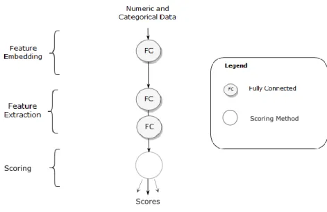
Deep-Learning Architecture Overview ... 23

Figure 6

–

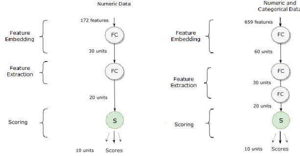
Architecture of Model 1 and 3 ... 25

Figure 7

–

Architecture of Model 2 ... 25

vi

LIST OF TABLES

Table 1

–

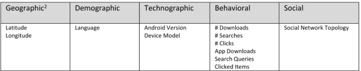
Features ... 28

Table 2

–

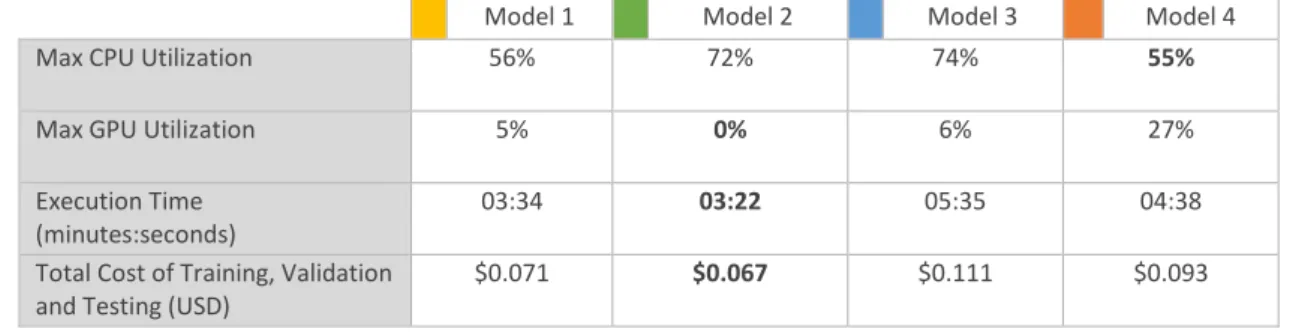
Computational Statistics of Model Training, Validation and Testing. ... 31

Table 3

–

Computational Statistics of Model Deployment ... 31

vii

LIST OF ABBREVIATIONS AND ACRONYMS

ALS Alternating Least Squares.

ANN Artificial Neural Network.

ARPU Average Revenue per User.

ASO App Store Optimization.

AUC Area Under the Receiver Operating Curve.

BB Beta-Binomial.

BG Beta-Geometric.

CBR Case-Based Reasoning.

CENE Content-Enhanced Network Representation Learning.

CF Collaborative Filtering.

CLV Customer Lifetime Value.

CRM Customer Relationship Management.

CTR Click Through Rate.

DMD Dirichlet Multinomial Distribution.

DNC Differentiable Neural Computer.

DNN Deep Neural Network.

E-Commerce Electronic Commerce.

FC Fully Connected.

GP-GPU General Purpose Graphics Processing Unit.

HDFS Hadoop Distributed File System.

IS Information Systems

IT Information Technology

KLR Kernel Logistic Regression.

KNN K-Nearest Neighbors.

viii

LDA Linear Discriminant Analysis.

LinReg Linear Regression.

LR Logistic Regression.

LSTM Long-Short Term Memory.

M-Commerce Mobile Commerce.

MLP Multilayer Perceptron.

MLR Multinomial Logistic Regression.

MSE Mean Squared Error.

M-KLR Multiclass Kernel Logistic Regression.

NBD Negative Binomial Distribution.

NRMSE Normalized Root Mean Squared Error.

PLS Partial Least Squares.

RBF Radial Basis Function.

RFF Random Fourier Features.

RFM Recency Frequency Monetary.

RMSE Root Mean Squared Error.

RNN Recurrent Neural Network.

ROC Receiver Operating Curve.

SEM Structural Equation Modeling.

SEO Search Engine Optimization.

SGD Stochastic Gradient Descent.

SVD Singular Value Decomposition.

1

1.

INTRODUCTION

It is often claimed that the internet changed the retail businesses. For the first-time retailers were not limited to an assortment of popular items and were able to profit from having an endless product variety (Brynjolfsson, Hu, & Smith, 2006). This implies that the aggregated demand for niche products is comparable to the top most popular products – a phenomenon known as the “long tail” effect (Anderson, 2008). Two main factors are usually suggested as the cause of this effect (Goel, Broder, Gabrilovich, & Pang, 2010): one related with the supply side (retailers/producers) and another related with the demand side (consumers).

On the supply side, online retailers can include an incredibly large number of items on their assortment when compared to traditional brick and mortar retailers (Brynjolfsson et al., 2006). This would theoretically be an advantage since demand is heterogeneous, and therefore a larger number of items would allow the retailer to provide more utility to a larger number of customers (Quan & Williams, 2017). Some empirical evidence of this has been found (Goel et al., 2010), suggesting that all consumers have a small portion of niche products in their choices. Also, in the context of digital goods distribution (which can include products such as apps, music, video and written content), advances in Cloud Computing also allowed for an almost linear scaling of data storage infrastructure, which is

necessary to attain extremely large assortments with “long-tail” properties (Weinhardt et al., 2009). On the consumer side, information search costs are hypothesized to be lower for consumers in the online context. By providing search engine and recommender system capabilities, users can more easily access the relevant content from the assortment (Schnabel, Bennett, & Joachims, 2018). In the particular case of mobile app stores, search engines have an increasingly key importance, as evidenced by the rising importance of App Store Optimization (ASO) for publishers in mobile app stores (Wilson, 2018). ASO refers to the tactics employed to improve visibility in app stores similarly to Search Engine Optimization (SEO) (Bilgihan, Kandampully, & Zhang, 2016). This appears to confirm that these systems do play a role in lowering information search costs for consumers. Several studies have provided evidence that recommender systems have a positive impact in content discovery in online environments (Brynjolfsson, Hu, & Simester, 2011; D. M. Fleder & Hosanagar, 2007; Pathak, Garfinkel, Gopal, Venkatesan, & Yin, 2010), which should reinforce the “long tail”.

While the impact of the “long tail” effect is usually considered very important for businesses, empirical

evidence suggests that this effect doesn’t occur in every digital market. In markets such as the online music industry, demand tends to follow a “Superstar” effect (Rosen, 1981), also referred to as the

“Winner-takes-all” (Frank Robert & Cook Philip, 1995) or “Blockbuster” (D. Fleder & Hosanagar, 2009) effect. In these markets, the demand for the most popular products largely exceeds the aggregated demand for the least popular ones. The mobile app economy has been found to behave in a similar manner (Zhong & Michahelles, 2013). This “Superstar” effect is consistent with marketing science

theory, since it can be explained by two other empirical generalizations that tend to occur across markets (Zhong & Michahelles, 2012, 2013): the natural monopoly effect and the double jeopardy law (A. Ehrenberg & Goodhardt, 2002; A. S. C. Ehrenberg, Goodhardt, & Barwise, 1990; A. S. C. Ehrenberg, Uncles, & Goodhardt, 2004). It has been argued that search engines and recommender systems are especially relevant for these markets (Yin, Cui, Li, Yao, & Chen, 2012; Zhong & Michahelles, 2013), as long as they are able to increase sales diversity.

2 Some authors argue that different methods of recommendation yield different levels of impact in search cost reduction and thus on sales diversity (D. Fleder & Hosanagar, 2009; D. M. Fleder & Hosanagar, 2007; Zhong & Michahelles, 2013). This suggests that “long tail” effects might be achieved

in “superstar” markets by having smarter recommender systems, or by avoiding the usual methods

based on collaborative filtering, which tend to reinforce the most popular items (Peltier & Moreau, 2012; Zhong & Michahelles, 2013).

While collaborative filtering was for a long time the main method of building recommender systems, several novel approaches have been proposed in recent years (Bobadilla, Ortega, Hernando, & Gutiérrez, 2013; Koutrika, 2018). Amongst these, deep-learning methods for recommendation systems have seen an exponential rise in published research and results suggest that they are capable of outperforming the traditional approaches (S. Zhang, Yao, & Sun, 2017). In particular, these methods have already been successfully employed in mobile app stores (Cheng et al., 2016). The traditional approaches based on collaborative filtering leverage memorization, but deep-learning has been shown to have a higher generalization capacity (Arpit et al., 2017), especially when regularization is applied, which results in more diverse recommendations (Cheng et al., 2016).

Additionally, we must consider the data sources used to train a recommendation model. The traditional approaches rely solely on either item-item or user-item similarities inferred through matrix factorization methods (Koutrika, 2018). Modern Deep Learning approaches can take advantage of all these features simultaneously. Deep Neural Networks (DNN) can detect non-linear relationships between all these signals (Goodfellow, Bengio, & Courville, 2016, p. 169), which is expected to further contribute to recommendation diversity.

Some early recommender engines relied on user ratings, which have been found not to be the best data source for effective recommender systems (Amatriain, 2013). In contrast, many online retailers, such as mobile app stores, have access to a wide variety of data, which includes user features (demographic, geographic, technographic and behavioral), user-generated content (comments, reviews and search queries), as well as content-based features (app descriptions, app usage and app download co-occurrence which can be used to infer implicit ratings and similarity). Additionally, some mobile app stores such as Google Play - in the past through its Google Plus integrations (Amadeo, 2016), currently through Google Play Games (Google, 2018a) and Google Play Family Library (Google, 2018b), and Aptoide - branded as the social app store, are augmented with online social network features (boyd & Ellison, 2007; Pallis, Zeinalipour-yazti, & Dikaiakos, 2011), which include microblogging, social networking, reviewing, commenting and messaging. Add to this the fact that these app stores run in mobile devices with constant connectivity, which adds real-time streaming characteristics to the data.

Given this context, we can argue that mobile app stores are dealing with data that possesses the 3V properties of Big Data (Sivarajah, Kamal, Irani, & Weerakkody, 2017): Volume, Velocity, and Variety. This suggests that app stores will require Big Data management technologies (which rely on distributed processing) to train, validate, test and deploy recommendation models. Traditional memory-based and matrix factorization approaches are hard to scale in the Big Data context, and we can only obtain approximate numerical solutions – see for instance these Apache Spark implementations of K-Nearest

3 Neighbors (Maillo, Ramírez, Triguero, & Herrera, 2017) and matrix factorization methods (Bosagh Zadeh et al., 2016). In contrast, DNN models are widely used in data-rich environments to process large amounts of unstructured data (Wedel & Kannan, 2016), and thus are a good fit for mobile app store recommender systems, since they are easier to train and deploy in a distributed manner (Alsheikh, Niyato, Lin, Tan, & Han, 2016).

A limitation of DNN is the fact that, since these do not rely on memorization, their response times are higher than the traditional approaches, which presents a problem in online production environments (Cheng et al., 2016). More complex models are costlier to train and deploy, thus a tradeoff must be made between precision and performance. Few studies have analyzed the cost-benefit of different DNN models, along with the impact of the data sources or the different scoring methods in the context of recommender systems.

A study by Cheng (2016) approached some of these questions while introducing Wide and Deep Learning architectures in mobile app store recommendations. However, the study didn’t evaluate the

economic impact of such a model. Also, while it did analyze the impact of using rich cross-product features, it didn’t analyze the impact of different feature augmentation methods (such as using only structured versus unstructured data) or the impact of not using embedding layer pretraining. Finally, it didn’t compare different scoring methods in the final layer (a softmax node was always employed). In this thesis, we intend to explore some of these open questions.

Our main objective is to determine the most efficient deep-learning based recommender system architecture for mobile app stores. To achieve this, we need to satisfy three specific objectives:

1. Assess the impact of using unstructured data versus only using structured data. 2. Assess the impact of embedding layer pre-training in the model performance. 3. Determine the efficiency of using Kernel-based methods in the scoring layer.

The efficiency should be measured using an economic profit metric. This metric should incorporate the estimated financial impact of improvements in customer experience. The improvement should be measured against a baseline, which can be estimated from natural monopoly and double jeopardy effects. Double jeopardy effects are regularly observed in online retail and e-commerce (Huang, 2011) and these appear to extend to m-commerce settings, in particular, the mobile app market, as we’ve

already seen (Zhong & Michahelles, 2013). Since these effects explain mobile app choice behavior and e-commerce in general, we can assume it explains mobile app store choice (at least in the Android platform), with public data confirming that a significant portion of Android users use third-party app stores other than Google Play (App Annie, 2017). Finally, the metric should also incorporate a holistic cost accounting of the model training, validation, testing and deployment at Big Data scale, including cloud computing costs.

In the following sections we will present a literature review covering Recommender Systems, Deep Learning and Big Data. Then we will describe the methodology employed to answer our research questions. Next, we will present the main results, followed by the conclusions, which include a discussion of the results and its implications, the limitations of the study and possible directions for future research.

4

2.

LITERATURE REVIEW

2.1.

R

S

Recommender systems attempt to solve the problem of information overload (Aljukhadar, Senecal, & Daoust, 2010). Humans have a limited cognitive ability, and thus, our brains evolved to have selective attention (Sayago, Guijarro, & Blat, 2012). It allows us to select the most relevant events or objects to focus our attention by taking clues from the environment. However, while the sapiens brain was well adapted to our ancestral environment, it is less adapted to modern digital environments (Huggett, Hoos, & Rensink, 2007), many times resulting in confusion (Sayago et al., 2012).

With the adoption of information systems (IS) in enterprises, information overload problems became increasingly common, triggering the need for recommender systems. As such, the first recommender system was Tapestry (Goldberg, Nichols, Oki, & Terry, 1992), an email filtering system developed at Xerox to deal with a large number of irrelevant emails received by employees. It was also the first time that the term Collaborative Filtering (CF) was employed, which to this day is still one of the most effective and widely used approaches to recommender system design (Su & Khoshgoftaar, 2009). Since then many well-known successful applications of recommender systems have appeared in major websites such as Amazon.com, YouTube, Netflix, Spotify, LinkedIn, Facebook, Tripadvisor, Last.fm, and IMDb (Ricci, Rokach, & Shapira, 2015).

Research in this field had its biggest boost due to the Netflix prize which had the first edition at the end of 2006 (Bennett & Lanning, 2007), and again in 2008 and 2009 (Grand Prize). The first and last events appear to have had the biggest impact on scientific production in the field, as evidenced from a bibliographic analysis of recommender system research on a 20-year period1 _{(Chart 1).}

Chart 1 – Number of research papers (with more than 10 citations) mentioning recommender systems between 1997 and 2017.

(Source: Google Scholar)

2.1.1.

Modeling Approaches

Recommender systems can leverage three types of similarities (Katsov, 2018, p. 275): User, Product, and Context. User similarities refer to using the attributes of each customer to infer their intent and

1_{The sample was collected from Google Scholar using Harzin’s PoP tool by searching for articles containing}

the phrase “recommender systems”. The analysis only includes papers with more than 10 citations.

0 100 200 300 400 500 600 700 1997 1998 1999 2000 2001 2002 2003 2004 2005 2006 2007 2008 2009 2010 2011 2012 2013 2014 2015 2016 2017

5 preferences. Product similarities refer to using the relationships between users and merchandise which can be expressed in different manners. Many early systems had a focus on explicit ratings, but these relationships can also be inferred through usage data for instance (as a binary variable indicating item consumption, or through counts) (Katsov, 2018, p. 276). CF traditionally leverages either user-based or product-user-based filtering, or both (hybrid filtering). Finally, context refers to additional signals related to the moment of purchase or the expressed intent (for instance by considering the season of the year). Usually, contextual data is used as a complement to more traditional CF tasks, either by pre-filtering or post-pre-filtering (Katsov, 2018, p. 289).

Another lesser-known type of recommender system includes Knowledge-based filtering (Burke, 2000), which takes advantage of Case-Based Reasoning (CBR) (González-Briones, Rivas, Chamoso, Casado-Vara, & Corchado, 2018). CBR works by asking the user a set of questions that allow the system to produce a recommendation based on previously defined rules. Like contextual recommender systems, CBR features are commonly integrated into recommender systems built with CF methods.

CF methods can further be divided into two types: memory based and model-based (Bobadilla et al., 2013).

Memory-based refers to using instance-based learning, such as K-nearest neighbors (KNN). KNN works by storing a matrix in memory (an instance) that relates users or users and items. For each new user, we take the 𝐾 nearest objects from the memory instance, using a previously chosen distance or similarity function 𝑓(𝑋𝑎, 𝑋𝑏) that takes the attributes 𝑋𝑎 and 𝑋𝑏 of each object 𝑎 and 𝑏 as input (Aha,

Kibler, & Albert, 1991). This distance measure might be Euclidean if the user/item features have metric properties. In that case 𝑓(𝑋𝑎, 𝑋𝑏) can be defined as:

𝑓(𝑋𝑎, 𝑋𝑏) = √∑(𝑋𝑎− 𝑋𝑏)2

Jaccard Distance is a common approach if the variables are binary. Under this distance metric we have (Torres, Skaf-Molli, Molli, & Díaz, 2013):

𝑓(𝑋𝑎, 𝑋𝑏) =

|𝑋𝑎∪ 𝑋𝑏| − |𝑋𝑎∩ 𝑋𝑏|

|𝑋𝑎∪ 𝑋𝑏|

In KNN, the value for 𝐾 is a hyper parameter. A common rule of thumb is to use the square root of the number of samples (Vrooman et al., 2007). The final recommendations can be based on the top most common items amongst the K-nearest neighbors, or by averaging (if we are working with explicit ratings).

Within model-based approaches, some authors identify two sub-categories (Katsov, 2018, p. 289): regression and latent factor methods.

Within latent factor methods, the most common method is Singular Value Decomposition (SVD). SVD is a matrix factorization technique that essentially performs dimensionality reduction on a user-user or user-item matrix. Mathematically, SVD is nothing more than a generalization of Gaussian elimination, which predated widespread usage of matrices (but is nevertheless consistent with what nowadays is referred to as generalized eigenvalue problem) to non-square and non-real matrixes

6 (Stewart, 1993). Suppose we have a real matrix 𝐴 with 𝑖 rows and 𝑗 columns, that represent the relationship between users and items, users and users, or users and their attributes.

Our goal is to obtain a decomposition of 𝐴, such that: 𝐴 = 𝑈Σ𝑉𝑇

𝑈 = (𝑢1, 𝑢2, … , 𝑢𝑖)

𝑉 = (𝑣1, 𝑣2, … , 𝑣𝑗)

Where Σ = 𝑑𝑖𝑎𝑔(𝜎1, 𝜎2, … 𝜎𝑛) has nonnegative diagonal elements arranged in descending order of

magnitude (the eigenvalues) and 𝑈 and 𝑉 are two matrices. The matrix 𝑈 contains the left eigenvectors, while 𝑉 contains the right eigenvectors (Gass & Rapcsák, 2004). If 𝐴 is a user by user matrix, 𝑈 = 𝑉. In cases where we have a user by attribute or user by item matrix, 𝑈 can be interpreted as the eigenvectors of the rows, while 𝑉 are the eigenvectors of the columns (which can be either items or user attributes). For the final analysis, we should select the relevant matrix of eigenvectors to use as the extracted eigenvectors (which can be either the left or the right depending on the definition of 𝐴 and the specific problem).

The extracted eigenvectors can be interpreted as latent factors that explain the variance or inertia (Greenacre, 1988) of either the rows or columns of 𝐴 . The variance or inertia of each factor is nothing more than the eigenvalue (an element of Σ) associated with that eigenvector. These extracted dimensions have metric properties and can then be used to estimate an Euclidean distance between objects before applying KNN. The alternative is to use these as input to another model to score items for a specific user. Several applications of SVD to recommender systems are known (Barragáns-Martínez et al., 2010; Brand, 2003; Paterek, 2007; Sarwar, Karypis, Konstan, & Riedl, 2000).

Other similar approaches based on latent factors include Matrix Factorization using Alternating Least Squares (ALS) and Stochastic Gradient Descent (SGD) learning algorithms (Koren, Bell, & Volinsky, 2009). These approaches are like SVD but tend to generalize better to new cases. This is so because the learning is done using a numerical optimization algorithm which is not only able to better deal with missing values but can also include a regularization term. In these approaches we may have a model as such:

𝑟̂𝑖𝑗= 𝑣𝑗𝑇𝑢𝑖+ 𝜇𝑖+ 𝑏𝑖+ 𝑏𝑗

Where 𝑟̂𝑖𝑗 is the predicted rating of item 𝑖 for user 𝑗, 𝑇 denotes the matrix transpose, 𝜇𝑖 is the average

rating of item 𝑖, 𝑏𝑖 and 𝑏𝑗 are bias terms for the item and user respectively. To perform the

optimization, we need to minimize a loss function such as the regularized squared error: 𝑅 = [ 𝑟11 ⋯ 𝑟1𝑗 ⋮ ⋱ ⋮ 𝑟𝑖1 ⋯ 𝑟𝑖𝑗 ] min 𝑣∗_,𝑢∗∑(𝑟𝑖𝑗− 𝜇 − 𝑏𝑖− 𝑏𝑗− 𝑣𝑗 𝑇_𝑢 𝑖)2+ 𝜆(∥ 𝑣𝑗∥2+∥ 𝑢𝑖 ∥2)

𝑅 is a matrix where each element 𝑟𝑖𝑗 indicates the rating of item 𝑖 for user 𝑗 and 𝜆(∥ 𝑣𝑗 ∥2+∥ 𝑢𝑖 ∥2) is

7 Within regression methods, Linear Regression (LinReg) is commonly employed as a baseline model when rating data is available (Mild & Natter, 2002). In the case of recommender systems we need to fit a LinReg model for each item 𝑗 as such:

𝑟̂𝑖𝑗 = 𝑣𝑗𝑇𝑢𝑖+ 𝑏𝑖

The standard method is based on ordinary least squares optimization. As such we can obtain estimates for the 𝑉̂ parameters using the OLS estimator:

𝑉̂ = (𝑈𝑇𝑈)−1𝑈𝑇𝑅

A key limitation of such methods is the fact that we can only work with rating data (either implicit or explicit). In cases where we only have binary data (for instance, about if a user either downloaded or not a certain app) we require a different modeling approach. The standard method for binary target variables is Logistic Regression (LR), but in this case, since we’re in a multilabel problem, we require Multinomial Logistic Regression (MLR), which can have two forms (Dow & Endersby, 2004): Logit (or Softmax) and Probit. Since logit models are more commonly employed in recommender systems our analysis will focus on these.

Let’s suppose we have a set of items 𝒮, a set of users ℛ and a choice matrix 𝐿 such that: 𝐿 = [

𝑙11 ⋯ 𝑙1𝑏

⋮ ⋱ ⋮

𝑙𝑎1 ⋯ 𝑙𝑎𝑏

]

Where each value of 𝐿 is 1 if a certain user 𝑎 ∈ ℛ chose item 𝑏 ∈ 𝒮 and 0 otherwise. Consider now the problem of estimating the probability 𝑃(𝐶𝑟,ℎ) of a new user 𝑟 ∈ ℛ choosing each item ℎ ∈ 𝒮, and that

this probability can be estimated from the vector of user attributes 𝑋𝑟 = [

𝑥𝑟1

⋮ 𝑥𝑟𝑘

]. The multinomial logit model then has the following specification (Aurier & Mejía, 2014):

Θ = [ 𝜃11 ⋯ 𝜃1𝑘 ⋮ ⋱ ⋮ 𝜃ℎ1 ⋯ 𝜃ℎ𝑘 ] 𝑌𝑟,ℎ= 𝑋𝑟[ 𝜃1 ⋮ 𝜃ℎ ] 𝑇 + 𝛼ℎ 𝑃(𝐶𝑟,ℎ) = 𝑒𝑌𝑟,ℎ ∑ 𝑒𝑌𝑟,𝑠 𝑠∈𝒮

Where 𝑌𝑟,ℎ is a measure of the utility of item ℎ for user 𝑟, θ is a matrix of parameters (weights) of each

user attribute for each item, and 𝛼ℎ is the constant utility for each item ℎ. We then apply the maximum

likelihood estimation method, which is based on cross-entropy loss minimization. The cross-entropy loss function has the following form (Christopher, 2006, p. 209):

𝐸(Θ) = − ∑ ∑ 𝑙𝑞,𝑤 ln 𝑃(𝐶𝑞,𝑤) 𝑤∈𝒮

8 A parameter estimate Θ̂ can be obtained in an iterative manner using the Newton-Raphson Method. At each iteration, we take the gradient of the error function in respect to one of the parameters 𝜃𝑝 to

update its value (Christopher, 2006, p. 210):

∇𝜃_𝑝𝐸(Θ) = ∑[𝑃(𝐶𝑞,𝑤) − 𝑞∈ℛ

𝑙𝑞,𝑤]𝑋𝑞

The final recommendations can be found by simply applying the following recommendation function 𝑔 to each value 𝑃(𝐶𝑞,𝑤):

𝑔(𝑥) = {1 𝑖𝑓 𝑥 > 0.5 0 𝑜𝑡ℎ𝑒𝑟𝑤𝑖𝑠𝑒 If 𝑔(𝑃(𝐶𝑞,𝑤)) = 1 we will recommend item 𝑤 for user 𝑞.

Several empirical applications of MLR to recommender systems are known (D. M. Fleder & Hosanagar, 2007; S.-H. Yang, Long, Smola, Zha, & Zheng, 2011; Zhao, Zhang, Zhang, & Friedman, 2016).

Many other modeling approaches exist for recommender systems. Fischer’s Linear Discriminant Analysis (LDA), also known as Multivariate Discriminant Analysis has been employed for recommender systems (K. Kim, 2011). Tree-based machine learning methods such as Decision Trees (Cho, Kim, & Kim, 2002; Gershman & Meisels, 2010), Random Forests (O’Mahony, Cunningham, & Smyth, 2010; H. R. Zhang & Min, 2016) and Gradient Boosted Regression Trees (Ostuni, Di Noia, Mirizzi, & Di Sciascio, 2014) have also been employed.

Bayesian methods were common approaches in the early 2000s (Condli, Madigan, Lewis, & Posse, 1999; Jin & Si, 2004; Miyahara & Pazzani, 2000). Towards the end of the decade some applications of ensemble methods emerged (Jahrer, Töscher, & Legenstein, 2010; Schclar, Tsikinovsky, Rokach, Meisels, & Antwarg, 2009) along with econophysics inspired approaches based on heat and mass diffusion techniques, which have reemerged recently (C. Liu & Zhou, 2010; Lü et al., 2012; Ren, Zhou, & Zhang, 2008; Vidmer, Zeng, Medo, & Zhang, 2015; Y. C. Zhang, Blattner, & Yu, 2007).

Kernel methods have also found applications in recommender systems (Abernethy, Bach, Evgeniou, & Vert, 2008; X. Liu et al., 2016) including the use of Support Vector Machines (SVM) (Fortuna, Fortuna,

& Mladenić, 2010; Oku, Nakajima, Miyazaki, & Uemura, 2006; Xia, Dong, & Xing, 2006).

Kernel methods are based on the kernel trick also known as kernel substitution (Christopher, 2006, p. 292). In these methods we do a mapping of the feature space of new unlabeled inputs 𝑥′ to the training examples 𝑥, using a kernel function 𝑘 that relies on a basis function 𝜑𝑞 such that:

𝑘(𝑥, 𝑥′) = 𝜑(𝑥)𝑇𝜑(𝑥′) = ∑ 𝜑𝑞(𝑥)𝜑𝑞(𝑥′) 𝑞∈ℛ

The basis function can assume several forms. The most commonly employed form is the Radial Basis Function (RBF) (Christopher, 2006, p. 299). Recently scalable approximation methods based on stochastic methods have emerged, such as Random Fourier Features (RFF) (Rahimi & Recht, 2007). Kernel methods can be seen as a form of instance-based methods, where the kernel function acts as a similarity measure between the training set and the new cases (Christopher, 2006, p. 292). These techniques allow us to linearize the feature space so that simpler decision algorithms can be employed.

9 The application of SVMs to recommender systems involves training an SVM classifier for either each user or each item (Xia et al., 2006). In either case, we are seeking to find a set of items to recommend to each user, by either classifying users for an item or vice-versa. We will assume that a model will be fit for each item, but the inverse specification works in a similar manner.

SVMs rely on the kernel mapping to obtain a transformed feature space where a linear decision boundary can be found based on the support vectors, which are sample cases that lie on the maximum margin hyperplanes in the feature space (Christopher, 2006, p. 330). This maximum margin hyperplane for an item 𝑤 ∈ 𝒮 can be found by solving (Christopher, 2006, pp. 327–330):

arg min

Θ,𝑏 {∑ 𝐸∞

([𝜃𝑞𝑘(𝑥, 𝑥𝑞) + 𝑏]𝑙𝑞,𝑤− 1) + 𝜆||Θ||2 𝑞∈ℛ

}

Where 𝐸∞(𝑧) is a function that returns 0 if 𝑧 ≥ 0 (which happens when the vector corresponding to 𝑞

is not a support vector), and ∞ otherwise. Alternative multiclass formulations of SVM have been proposed (Hsu & Lin, 2002), which could be used to jointly train a classifier across all items, but no recommender system applications are yet known. Similar methods exist with could potentially be employed to build recommender systems, such as Kernel Logistic Regression (KLR). KLR differs from LR in the definition of 𝑌𝑟,ℎ: 𝑌𝑟,ℎ= 𝑘(𝑋, 𝑋𝑟) [ 𝜃1 ⋮ 𝜃ℎ ] 𝑇 + 𝛼ℎ

A multilabel version of KLR can be achieved by performing the same substitution with softmax instead of LR as in Karsmakers, Pelckmans, & Suykens (2007). KLR has been empirically and analytically demonstrated as having the similar performance and behavior of an SVM (Karsmakers et al., 2007), the main difference being the fact that it requires the entire dataset as opposed to only using the support vectors to build a decision margin (Zhu & Hastie, 2005). As such, it is expected that multiclass KLR should behave similarly to multiclass SVM approaches (Karsmakers et al., 2007). Currently, no applications of KLR (or its multiclass version) are known in recommender systems, but it can potentially improve existing LR/Softmax based methods.

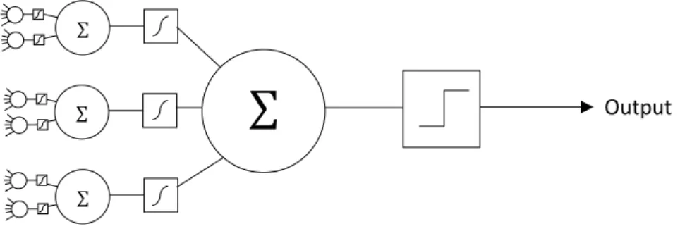
Other recommender systems techniques include Artificial Neural Networks (ANN), such as Multilayer Perceptrons (MLP), also known as shallow networks (Goga, Kuyoro, & Goga, 2015). The current state of the art in recommender system design is deep learning methods, which are deep versions of ANN (Cheng et al., 2016; Covington, Adams, & Sargin, 2016; Koutrika, 2018; H. Wang, Wang, & Yeung, 2015; S. Zhang et al., 2017). Both deep and shallow networks can have multiple output nodes that function like either multinomial linear regression or multinomial logistic regression.

2.1.2.

Model Evaluation

Model evaluation in the context of recommender systems includes several different metrics which range from multiclass/multilabel versions of traditional machine learning and data mining ones to specific profit-centric indicators (Gilotte, Calauzènes, Nedelec, Abraham, & Dollé, 2018; Ju, Choi, Kim, & Moon, 2017).

10 We can divide the evaluation metrics into three main groups: Offline, Online and User Studies (Beel & Langer, 2013).

Offline evaluation metrics are the most commonly employed. It assumes that models can be evaluated in terms of prediction/classification accuracy of past item consumption data or ratings. In this context, if an item is recommended to a user who hasn’t previously consumed it, we count it as a model failure.

It’s easy to see that offline metrics are not guaranteed to be realistic, since the fact that an item wasn’t previously consumed or rated, doesn’t mean it’s not relevant to that user.

Online metrics can overcome these issues by testing the recommender system in a production environment. In this context we can apply several specific recommender system metrics, usually derived from marketing evaluation metrics applied in online advertising and e-commerce (Beel & Langer, 2013). The most common metric is the Click-Through Rate (CTR) (Beel & Langer, 2013):

𝐶𝑇𝑅 = 𝐶𝑙𝑖𝑐𝑘𝑠

𝐼𝑚𝑝𝑟𝑒𝑠𝑠𝑖𝑜𝑛𝑠

Where impressions are the number of impressions of all recommended items, and clicks are the number of items that were clicked after being recommended. The assumption of this metric is that a clicked item is relevant to the user. While this assumption is not completely realistic, we can argue that its closer to reality than most offline evaluation metrics.

User studies come from the usability and user experience research tradition, which employ survey-based methods. Several standardized psychometric constructs exist to evaluate recommender systems. The ResQues framework proposed by Pu and Chen (2010) includes several constructs that can be measured individually using Factor Analysis or jointly using Structural Equation Modeling (SEM) with either Partial Least Squares (PLS) or Covariance-based estimation (Ayeh, Au, & Law, 2013). These constructs are related to user-perceived qualities, user beliefs, user attitudes and behavioral intentions (Pu & Chen, 2010). Other similar frameworks based on SEM have been proposed such as the Knijnenburg, Willemsen, Gantner, Soncu, & Newell (2012) model which can be used to measure the subjective user experience of a recommender system. These latent psychometric constructs can be used to compare different recommendation models from the point of view of the end-user experience.

We will focus on Offline evaluation since that’s the most common approach. Offline evaluation can be thought of as either a classification or a regression (prediction) problem, depending on the type of target variable we have (Herlocker, Konstan, Terveen, & Riedl, 2004). In the former, we are usually working with binary item consumption, while on the latter, we are usually working with explicit or implicit ratings.

Regression-type metrics for recommender system evaluation include the Mean Squared Error (MSE), Root Mean Squared Error (RMSE) and Normalized Root Mean Squared Error (NRMSE) (Katsov, 2018, p. 282). In these metrics, we are assuming that the model outputs a prediction 𝑦̂𝑟,ℎ for actual rating

𝑦𝑟,ℎ by user 𝑟 for item ℎ, resulting in an error term 𝑒𝑟,ℎ such that:

𝑒𝑟,ℎ= 𝑦̂𝑟,ℎ− 𝑦𝑟,ℎ

11 𝑀𝑆𝐸 = 1 |𝑇| ∑ 𝑒 2 𝑟,ℎ (𝑟,ℎ)∈𝑇

Where 𝑇 is a matrix of unseen user ratings for items used for model testing. MSE is not always

convenient because its value cannot be easily compared with the original ratings, since it’s a squared

value (Katsov, 2018, p. 282). RMSE allows us to overcome this issue: 𝑅𝑀𝑆𝐸 = √𝑀𝑆𝐸

RMSE was the target metric for the Netflix prize (Bennett & Lanning, 2007), and is currently the most popular choice for regression type model evaluation (Szabó, Póczos, & Lőrincz, 2012). NRMSE can now be defined as:

𝑁𝑅𝑀𝑆𝐸 = 𝑅𝑀𝑆𝐸

𝑦𝑚𝑎𝑥− 𝑦𝑚𝑖𝑛

The advantage of NRMSE is that its value is defined in the range (0,1), which allows us to compare models applied to ratings with different scales.

For classification type models we can employ multiclass/multilabel versions of traditional classification metrics, which can usually be done by macro (across classes) or micro (across cases) averaging (Tsoumakas & Vlahavas, 2007). Consider a binary evaluation measure 𝑀(𝑡𝑝, 𝑡𝑛, 𝑓𝑝, 𝑓𝑛) that is calculated based on the number of true positives (𝑡𝑝), true negatives (𝑡𝑛), false positives (𝑓𝑝) and false negatives (𝑓𝑛). Let 𝑡𝑝𝜌, 𝑓𝑝𝜌, 𝑡𝑛𝜌 and 𝑓𝑛𝜌 be the number of true positives, false positives, true

negatives and false negatives after binary evaluation for a label 𝜌. The macro-averaged and micro-averaged versions of 𝑀, are calculated as follows, where 𝐿 is the set of labels (items) (Tsoumakas & Vlahavas, 2007): 𝑀𝑚𝑎𝑐𝑟𝑜 = 1 |𝐿|∑ 𝑀(𝑡𝑝𝜌, 𝑓𝑝𝜌, 𝑡𝑛𝜌, 𝑓𝑛𝜌) |𝐿| 𝜌=1 𝑀𝑚𝑖𝑐𝑟𝑜= 𝑀(∑ 𝑡𝑝𝜌 |𝐿| 𝜌=1 , ∑ 𝑓𝑝𝜌 |𝐿| 𝜌=1 , ∑ 𝑡𝑛𝜌 |𝐿| 𝜌=1 , ∑ 𝑓𝑛𝜌 |𝐿| 𝜌=1 )

A popular metric for recommender system evaluation is the F1-Score (Herlocker et al., 2004) which can be defined based on the values of precision and recall:

𝑃𝑟𝑒𝑐𝑖𝑠𝑖𝑜𝑛 = 𝑡𝑝 𝑡𝑝 + 𝑓𝑝 𝑅𝑒𝑐𝑎𝑙𝑙 = 𝑡𝑝 𝑡𝑝 + 𝑓𝑛 𝐹1 𝑆𝑐𝑜𝑟𝑒 = 2 𝑃𝑟𝑒𝑐𝑖𝑠𝑖𝑜𝑛 × 𝑅𝑒𝑐𝑎𝑙𝑙 𝑃𝑟𝑒𝑐𝑖𝑠𝑖𝑜𝑛 + 𝑅𝑒𝑐𝑎𝑙𝑙

Where 𝑡𝑝 is the number of true positives (number of relevant recommendations), 𝑓𝑝 is the number of false positives (number of irrelevant recommendations) and 𝑓𝑛 is the number of false negatives (number of would be relevant items that were not recommended). Logically, and for the sake of completeness, we can further define an additional measure 𝑡𝑛 as the number of true negatives

12 (number of would be irrelevant items that were not recommended). These evaluation metrics usually assume an offline evaluation setting.

The most common metric for classification type models is the AUC (Verbeke, Dejaeger, Martens, Hur, & Baesens, 2012):

𝐴𝑈𝐶 = ∫ 𝐹0(𝑠)𝑓1(𝑠)𝑑𝑠 +∞

−∞

AUC assumes that a classifier produces a score 𝑠 = 𝑠(𝑥) from the features 𝑥 with a corresponding probability density function of these scores for class 𝑘 instances 𝑓𝑘(𝑠) and cumulative distribution

function 𝐹𝑘(𝑠) with two classes 𝑘 = 0,1. This metric can only be employed to evaluate models that

produce probability scores such as softmax regression.

Other related metrics are also used including the Gini coefficient (𝐺𝑖𝑛𝑖 = 2 × 𝐴𝑈𝐶 − 1) and the Kolmogorov-Smirnov (KS) statistic which is the maximum distance between a receiver operating curve (ROC) and the diagonal at a specific cut-off value (usually 0.5) (Verbeke et al., 2012).

An empirical study by Forman and Scholz (2009) advises the use of “average AUC” (consistent with the

previous definition of a Macro measure) and the “F1-Score computed from false and true positives”

(consistent with the previous definition of a Micro measure) to compute multilabel versions of AUC and F1-Score respectively.

Other popular multiclass classification metrics commonly employed to evaluate recommender systems include the Hamming loss and the Jaccard Index. Hamming loss can be defined as the proportion of misses (Luaces, Díez, Barranquero, del Coz, & Bahamonde, 2012):

𝐻𝑎𝑚𝑚𝑖𝑛𝑔 𝐿𝑜𝑠𝑠 = 𝐹𝑃 + 𝐹𝑁

𝐹𝑃 + 𝐹𝑁 + 𝑇𝑃 + 𝑇𝑁

Jaccard Index can be interpreted as a multilabel measure of accuracy based on the already defined Jaccard Distance (Luaces et al., 2012):

𝐽𝑎𝑐𝑐𝑎𝑟𝑑 𝐼𝑛𝑑𝑒𝑥 = 𝑇𝑃

𝐹𝑃 + 𝐹𝑁 + 𝑇𝑃

Additional evaluation metrics include Diversity, Coverage, Serendipity and Novelty (Katsov, 2018, pp. 285–288), which originate from desirable recommender system properties (Ge, Delgado-Battenfeld, & Jannach, 2010; Vargas & Castells, 2011). Most of these might be applied in both offline and online settings. We will review some of the most common measurement approaches.

Diversity is the ability of the recommender system to produce recommendations that are dissimilar (Katsov, 2018, p. 286). To measure diversity, we need to leverage a content-based similarity metric.

One approach is to extract features from the item’s description/title (using text mining and natural

language processing techniques), contents (requiring some form of feature extraction from multimedia/hypermedia content), or some other properties.

In alternative, we can also obtain a similarity metric between items by factorizing a user by items matrix

with the methods we’ve already seen (such as memory-based methods, SVD or even knowledge-based

13 𝑠𝑖𝑚𝑖𝑙𝑎𝑟𝑖𝑡𝑦(𝑎, 𝑏) ∈ [0,1]

𝑑𝑖𝑠𝑡(𝑎, 𝑏) = 𝑑𝑖𝑠𝑡(𝑏, 𝑎) = 1 − 𝑠𝑖𝑚𝑖𝑙𝑎𝑟𝑖𝑡𝑦(𝑎, 𝑏)

The diversity of the set of recommendations for each user can then be defined as the average distance between all pairs of recommendations.

Coverage refers to the percentage of users that the recommender system can give recommendations to (Katsov, 2018, p. 289). This is important because of the sparse nature of the data for recommender systems, which is also the source of the cold start problem (Schein, Popescul, Ungar, & Pennock, 2002). Another view on coverage is related to catalog coverage which is the percentage of the catalog merchandise that is being recommended (Katsov, 2018, p. 289):

𝐶𝑎𝑡𝑎𝑙𝑜𝑔 𝐶𝑜𝑣𝑒𝑟𝑎𝑔𝑒 = 1

|𝒮||⋃ 𝑌𝑢

𝑢∈ℛ

|

Where 𝑌𝑢 is a recommendation list for user 𝑢, |𝒮| is the cardinality of the set of items 𝒮 and ℛ is the

set of all users.

Serendipity is a measure of the extent to which recommendations are attractive and surprising (Katsov, 2018, p. 286). Despite being subjective, heuristic approaches have been suggested based on baseline models that produce trivial recommendations (Ge et al., 2010), which are usually simple recommendation system approaches. From that baseline, we will create a set of expected items. Any

item that doesn’t belong to this set will be considered unexpected. We can define a usefulness function

that returns 1 when a given recommendation is both relevant and unexpected. Serendipity is therefore defined as:

𝑆𝑒𝑟𝑒𝑛𝑑𝑖𝑝𝑖𝑡𝑦 =∑𝑖𝑡𝑒𝑚 ∈ 𝒮𝑈𝑠𝑒𝑓𝑢𝑙𝑛𝑒𝑠𝑠(𝑖𝑡𝑒𝑚) |𝒮|

Recommendations are considered novel if the user is not aware of the recommended items at the moment the recommendation is provided (Katsov, 2018, p. 285). Many approaches exist to measure novelty: Popularity-based, Distance-based (Vargas & Castells, 2011) and Time-based (Katsov, 2018, p. 285). Popularity-based novelty measurement takes advantage of the long-tail concept. If a relevant recommended item is less popular, we can assume that it might be more novel. Therefore (Vargas & Castells, 2011):

𝑁𝑜𝑣𝑒𝑙𝑡𝑦𝑃𝑜𝑝𝑢𝑙𝑎𝑟𝑖𝑡𝑦−𝑏𝑎𝑠𝑒𝑑(𝑖𝑡𝑒𝑚, 𝑐𝑜𝑛𝑡𝑒𝑥𝑡) = 1 − 𝑝(𝑠𝑒𝑒𝑛|𝑖𝑡𝑒𝑚, 𝑐𝑜𝑛𝑡𝑒𝑥𝑡)

Distance-based novelty measurement takes advantage of the item features to define a distance measure between items. Then we can leverage the user’s past behavior to measure how novel that

item might be for a specific user, by considering its past consumption context. Therefore (Vargas & Castells, 2011):

𝑁𝑜𝑣𝑒𝑙𝑡𝑦𝐷𝑖𝑠𝑡𝑎𝑛𝑐𝑒−𝑏𝑎𝑠𝑒𝑑(𝑖𝑡𝑒𝑚, 𝑢𝑠𝑒𝑟) =_{𝑝𝑎𝑠𝑡 𝑖𝑡𝑒𝑚 ∈ 𝑢𝑠𝑒𝑟}min [1 − 𝑠𝑖𝑚𝑖𝑙𝑎𝑟𝑖𝑡𝑦(𝑖𝑡𝑒𝑚, 𝑝𝑎𝑠𝑡 𝑖𝑡𝑒𝑚)]

Time-based novelty measurement assumes that the elapsed time between recommendation and action taken on that item by a user indicates its novelty level (Katsov, 2018, p. 285). A larger elapsed time means a higher novelty. Therefore:

14 𝑁𝑜𝑣𝑒𝑙𝑡𝑦𝑇𝑖𝑚𝑒−𝑏𝑎𝑠𝑒𝑑(𝑡𝑖𝑡𝑒𝑚) = 𝛾𝑡𝑖𝑡𝑒𝑚

Where 𝑡𝑖𝑡𝑒𝑚 is the elapsed time between the recommendation of the item and the action, and 𝛾 is a

time weight parameter. The weight parameter can either be set manually based on the retailer’s

experience, or empirically by combining past behavioral data with a user-based novelty psychometric construct (Pu, Chen, & Hu, 2012). We can therefore use a regression model to estimate the parameter, by assuming that the following relationship is true:

𝑁𝑜𝑣𝑒𝑙𝑡𝑦𝑈𝑠𝑒𝑟−𝑏𝑎𝑠𝑒𝑑(𝑖𝑡𝑒𝑚) = 𝛾𝑡𝑖𝑡𝑒𝑚

This novelty measurement approach overlaps with the user studies evaluation approach. In e-commerce settings we can also evaluate the recommender system using profit metrics derived from sales:

𝑃𝑟𝑜𝑓𝑖𝑡 = ∑ 𝑄𝑢𝑎𝑛𝑡𝑖𝑡𝑦 𝑆𝑜𝑙𝑑𝑖𝑡𝑒𝑚× 𝑀𝑎𝑟𝑔𝑖𝑛𝑖𝑡𝑒𝑚 𝑖𝑡𝑒𝑚𝑠

In environments where we are not selling items (including email, news, multimedia content recommendations, amongst others) this metric cannot be used. In the case of mobile app recommendations, most apps are free to download (94.24% in the Android platform, 88.18% in iOS) (Statista, 2018), which means that this metric can only be used for the small proportion of paid apps. For non-paid items, we need to consider a different approach to profit measurement based on the impact of the recommender system on the Customer Lifetime Value (𝐶𝐿𝑉) (Iwata, Saito, & Yamada, 2008). CLV is commonly used to guide Customer Relationship Management (CRM) processes (Blattberg, Kim, & Neslin, 2008, p. 163).

The revenue associated with each successfully recommended item is the portion of the 𝐶𝐿𝑉 that can be attributed to that item. Assuming that the revenue associated with each item is constant for all items, then the portion of the 𝐶𝐿𝑉 attributed to each item can be derived from the item consumption probability (Iwata et al., 2008). In environments such as mobile app stores, users can perform several different actions, but all of these are ultimately related with app consumptions, therefore its plausible to assume that app acquisitions are the major component of the 𝐶𝐿𝑉, and that these are heavily influenced by recommender systems.

𝐶𝐿𝑉 can be calculated using several methods. Traditionally 𝐶𝐿𝑉 would be estimated using a Recency, Frequency and Monetary (RFM) model to rank users (Gupta et al., 2006). Modern approaches extend the concept of RFM to obtain a financial estimation of the 𝐶𝐿𝑉 for each customer.

One approach to obtaining a global average of 𝐶𝐿𝑉 is to calculate the average of all individual-level 𝐶𝐿𝑉 values across a database, where the 𝐶𝐿𝑉 for each customer is given by (Blattberg et al., 2008, p. 108):

𝐶𝐿𝑉 = ∑(𝐷̃𝑡− 𝐶𝑡)𝑆𝑡 (1 + 𝛿)𝑡−1 ∞

𝑡=1

Where 𝛿 is the discount rate per time unit 𝑡, 𝐷̃𝑡 is the revenue generated by the user on moment 𝑡,

15 moment 𝑡. The RFM model is incorporated into 𝐶𝐿𝑉 through the 𝑆𝑡(“recency” and “frequency”) and

𝐷̃𝑡(“monetary”).

Several methods to obtain 𝐷̃𝑡 have been proposed (Blattberg et al., 2008, pp. 130–131): The simplest

approach is to assume that 𝐷̃𝑡 is constant in all periods based on the individual average or the global

Average Revenue Per User (ARPU). Trend, causal (based on the user features) and stochastic models are also commonly employed.

To model 𝑆𝑡= 𝑝(𝑎𝑙𝑖𝑣𝑒) we need a consumer behavior model. Several have been proposed: Beta

Binomial/NBD (BB-NBD) (Jeuland, Bass, & Wright, 1980), NBD-Dirichlet (Goodhardt, Ehrenberg, & Chatfield, 1984), Pareto/NBD (P-NBD) (Schmittlein, Morrison, & Colombo, 1987), Beta-Geometric/Beta-Binomial (BG-BB) (Fader, Hardie, & Berger, 2004), and Beta-Geometric/NBD (BG-NDB) (Fader, Hardie, & Lee, 2005). We will focus our attention on the most recent model by Fader et al.

(2005), according to which 𝑝(𝑎𝑙𝑖𝑣𝑒) is given by (Fader & Hardie, 2008): 𝑝(𝑎𝑙𝑖𝑣𝑒|𝑥, 𝑡𝑥, 𝑇, 𝑟, 𝛼, 𝑎, 𝑏) =

1 1 +_{𝑏 + 𝑥}𝑎 (_{𝛼 + 𝑡}𝛼 + 𝑇

𝑥) 𝑟+𝑥

Where 𝑥 is the number of transactions observed in the time-period (0, 𝑇](“frequency”) and 𝑡𝑥(0 <

𝑡𝑥 ≤ 𝑇) is the time of the last transaction (“recency”). The model’s four parameters 𝑟, 𝛼, 𝑎, 𝑏 can be estimated using maximum likelihood estimation from the likelihood function:

𝐿(𝑟, 𝛼, 𝑎, 𝑏 |𝑋 = 𝑥, 𝑡𝑥, 𝑇) =𝐵(𝑎, 𝑏 + 𝑥) 𝐵(𝑎, 𝑏) 𝛤(𝑟 + 𝑥)𝛼𝑟 𝛤(𝑟)(𝛼 + 𝑇)𝑟+𝑥 + 𝛿𝑥>0 𝐵(𝑎 + 1, 𝑏 + 𝑥 − 1) 𝐵(𝑎, 𝑏) 𝛤(𝑟 + 𝑥)𝛼𝑟 𝛤(𝑟)(𝛼 + 𝑡𝑥)𝑟+𝑥

Suppose we have a sample of 𝑁 customers, where customer 𝑖 had 𝑋𝑖 = 𝑥𝑖 transactions in the period

(0, 𝑇𝑖], with the last transaction occurring at 𝑡𝑥𝑖. The sample log-likelihood function is:

𝐿𝐿(𝑟, 𝛼, 𝑎, 𝑏) = ∑ 𝑙𝑛 𝐿(𝑟, 𝛼, 𝑎, 𝑏 |𝑋𝑖 = 𝑥𝑖, 𝑡𝑥𝑖 , 𝑇𝑖) 𝑁

𝑖=1

By maximizing this function using standard optimization methods, we can obtain the parameter estimates. While BG/NBD model and its extensions are the current state of the art, it requires individual-level data to estimate the parameters. The already mentioned NBD-Dirichlet model (Goodhardt et al., 1984) can be an alternative to this model with simpler data requirements.

NBD-Dirichlet results from the combination of two distributions: the Negative Binomial Distribution (NBD) and the Dirichlet Multinomial Distribution (DMD) (Dawes, Meyer-Waarden, & Driesener, 2015). The NBD part describes the category buying behavior of individuals in a market, while the DMD part models the probability of each individual in the market purchasing a specific brand (Goodhardt et al., 1984). The resulting model is therefore given by (Goodhardt et al., 1984):

𝑝(𝑟𝑗|𝑛) =

(_𝑟𝑛

𝑗) Β(𝛼𝑗+ 𝑟𝑗, 𝑆 − 𝛼𝑗+ 𝑛 − 𝑟𝑗)

16 Where 𝑝(𝑟𝑗|𝑛) can be interpreted in the context of online retail as the probability of using 𝑟𝑗 times the

retailer 𝑗 amongst 𝑛 usages of the retailer category, 𝛼𝑗 is the usage propensity for retailer 𝑗, 𝑆 is the

diversity of usage behavior in the category (𝑆 = ∑ α𝑗 𝑗) (Bound, 2009). We can assume that 𝑀𝑆𝑗= 𝛼𝑗/𝑆

where 𝑀𝑆𝑗 is the market share of the retailer 𝑗 (Wright, Sharp, & Sharp, 2002).

Β is the Beta function such that:

Β(𝑝, 𝑞) =Γ(𝑝)Γ(𝑞) Γ(𝑝 + 𝑞) Γ is the Gamma function such that:

Γ(𝑥) = ∫ 𝑡𝑥−1𝑒−𝑡𝑑𝑡, 𝑥 > 0

∞ 0

Accurate estimates for all 𝛼𝑗 can be obtained by fitting the DMD for all retailers 𝐽 in the market using

panel data such that (Wrigley & Dunn, 1985): 𝑝(𝑟1, 𝑟2, … , 𝑟𝑗|𝑛) = ( 𝑛 𝑟1, 𝑟2, … , 𝑟𝑗 ) Γ(𝑆) Γ(𝑆 + 𝑛)∏ [ Γ(𝛼𝑗+ 𝑟𝑗) Γ(𝛼𝑗) ] 𝐽 𝑗=1

Model estimation can be done using the original “mean and zero” method proposed by Goodhardt

(1984) or maximum likelihood (Wrigley & Dunn, 1985). Intelligence providers such as App Annie and 42Matters provide app usage intelligence data for the mobile industry, which can be used to estimate these parameters for all platforms. An Excel workbook is available to facilitate the model estimation using maximum likelihood (Rungie, 2003).

An R package is also available (F. Chen, 2016) which can be used to obtain estimates of 𝑆 by having as input the platform category penetration (category users in the population), platform penetration (users of the specific platform in the population), category usage frequency and the market shares of the different platforms. We can then obtain the platform usage propensity through its market share (𝑀𝑆𝑗= 𝛼𝑗/𝑆). The required input information can be found though several industry publications and

market intelligence providers such as Statista and GSMA Mobile Economy.

Under this set of assumptions 𝑝(𝑎𝑙𝑖𝑣𝑒) is 𝑝(𝑟𝑗> 0|𝑛), where 𝑛 is the average usage frequency of the

retailer category. NBD-Dirichlet is a realistic assumption, since online consumer behavior in the context of mobile app stores has been shown to follow the Double Jeopardy Law and Natural Monopoly effects described by the NBD-Dirichlet model (Zhong & Michahelles, 2013).

2.1.3.

Feature Extraction

As we’ve seen, model-based approaches to recommender system design can leverage several types of

user and context features. We will review some of the most common feature extraction techniques that are relevant for recommender system design in the context of online retailing. Given its social nature, many online retailers generate large amounts of user-generated content (such as comments, reviews, ratings, and likes), keyword search data, social network data. Its interactive and mobile features also generate behavioral data (such as touchstream/clickstream data), geographic coordinate data and technographic (device-related) data.

17 Behavioral data (touchstream/clickstream) along with technographic data, is usually more structured and easier to quantify. However, in Big Data context also becomes difficult to manage, and may require feature extraction techniques to reduce its dimensionality. Classic autoencoders are widely used for this purpose (Hinton & Salakhutdinov, 2006). Autoencoders are based on the Restricted Boltzmann Machine algorithm, which can be interpreted as a two-layer neural network (a visible and a hidden layer) where each unit takes a binary value ∈ [0,1]. The nodes from the visible layer serve as input to the hidden layer. The energy of a Boltzmann machine with 𝑁 nodes is defined by (Osogami, 2017):

𝐸𝜃(𝑥) = − ∑ 𝑏𝑖𝑥𝑖 𝑁 𝑖=1 − ∑ ∑ 𝑤𝑖,𝑗𝑥𝑖𝑥𝑗 𝑁 𝑗=𝑖+1 𝑁−1 𝑖=1

Where 𝑥 is a random configuration of binary states for the nodes, 𝑏𝑖 is its bias, 𝑤𝑖,𝑗 is the weight

between a pair of nodes 𝑖 and 𝑗. The parameters are collectively denoted by 𝜃 = (b1, . . . , b𝑁, w1,2, . . . , w𝑁−1,𝑁)

From the energy we can obtain a probability distribution over binary patterns (Osogami, 2017): 𝑃𝜃(𝑥) =

𝑒𝑥𝑝 (−𝐸𝜃(𝑥))

∑ 𝑒𝑥𝑝 (−𝐸𝜃(𝑥̃))𝑥̃

Where the summation with respect to 𝑥̃ is over all possible 𝑁 bit binary values. By optimally setting the values of 𝜃, we can approximate 𝑃𝑡𝑎𝑟𝑔𝑒𝑡(. ) with 𝑃𝜃(. ), meaning that we can reconstruct an input

from a compressed representation. Hinton (2006) demonstrated that Autoencoders have superior reconstruction power when compared to Principal Components Analysis (PCA), the most commonly used dimensionality reduction method. Thus, numerical data inputs can effectively be reduced to a smaller number of orthogonal features.

From the types of data previously described, user-generated content and keyword search data are unstructured. Before this data can be operationalized, we need to somehow quantify this data. Autoencoder inspired feature extraction methods have been proposed for this, such as Doc2Vec (Le & Mikolov, 2014). This method, in turn, is based on a previous word embedding method called Word2Vec (Mikolov, Chen, Corrado, & Dean, 2013). Word2Vec consists of a softmax regression model that predicts

w

w

𝑝(𝑤𝑖|𝑤𝑗) = 𝑒𝑥𝑝(𝑢𝑤⊤_𝑖𝑣𝑤 𝑗) ∑ 𝑒𝑥𝑝(𝑢𝑙 ⊤_𝑣 𝑤𝑗) 𝑉 𝑙=1

𝑢𝑤_𝑖− vector representation of the word 𝑊𝑖

𝑣𝑤_𝑗− vector representation of the word 𝑊𝑗

The resulting model allows us to assess which of the V are closest in the semantic space using this cosine distance (the probability of co-occurrence given by the model). If two words are close they can be considered to have identical meanings, which in linguistic terms equals being synonyms. Doc2Vec extends this very same methodology to documents.

18 Some mobile app stores possess social follower features, resulting in social network data. Social network data is also not structured in the traditional relational database sense, which makes it difficult to represent in SQL tables. Therefore, we can assume that social network data is semi-structured. Its quantification traditionally requires social network analysis techniques, that are usually performed on the entire graph. Popular hand-crafted node-level features include centrality measures (Bloch, Jackson, & Tebaldi, 2016) such as degree (indegree and outdegree), closeness, betweenness, eigenvector, Katz, PageRank, diffusion, and percolation (Piraveenan, Prokopenko, & Hossain, 2013). These social network features have had some applications in recommender systems (Li, Wu, & Lai, 2013). Other more general methods of feature extraction, based on Word2Vec and Random Walk sampling have been proposed such as DeepWalk (Perozzi, Al-Rfou, & Skiena, 2014). DeepWalk, like PageRank, is a very efficient technique for social network feature extraction at Big Data scale, while also having the advantage of providing general features which can be potentially more useful for recommender systems. Random walks are generated for each starting node, resulting in text sentences, whose features can be extracted using Word2Vec. Recently, a more general framework has emerged from DeepWalk, called Content-enhanced Network Representation Learning, or CENE (Sun, Guo, Ding, & Liu, 2016). This new method allows us to extract features from social graphs where each node is associated with textual content (with the possibility of also being extended to other types of multimedia content).

The feature extraction techniques previously mentioned are useful in extracting orthogonal features in the online retail context. Deep learning methods are currently the state of the art in recommender system design, that can leverage all these features to produce recommendations.

2.2.

D

L

Deep Learning refers to a specific type of artificial neural network models, capable of performing feature extraction as well as feature processing (LeCun, Bengio, & Hinton, 2015). Thus, deep learning can be defined in opposition to shallow learning, which refers to single data processing layer, a category that includes most traditional machine-learning methods (LeCun et al., 2015), but it’s usually employed to refer to traditional ANNs. While shallow models have been theoretically demonstrated as being capable of performing the same tasks as deep models (Cybenko, 1989; Leshno, Lin, Pinkus, & Schocken, 1993), recent research has revealed that to approximate the same functions a very wide shallow network with an exponentially larger number of nodes may be required (Montúfar, Pascanu, Cho, & Bengio, 2014). These results suggest that deep learning networks may be the only feasible option for efficient approximation with finite datasets in complex nonlinear systems (Goodfellow et al., 2016, p. 198).

As we’ve seen, deep learning originated from shallow learning, which usually means ANNs. These models originated from computational neuroscience, as a method of modeling the behavior of neurons. The first model of its type was the perceptron (Rosenblatt, 1958). This type of model simulates the behavior of the dendrites (neuron inputs), each with different weights, meant to model the effects of long-term potentiation and depression needed for plasticity and learning in the brain (Michmizos, Koutsouraki, Asprodini, & Baloyannis, 2011). The perceptron algorithm then simulates the neuronal response by either outputting -1 or 1 (meant to model neuronal spikes) if a given threshold is reached.

19 Figure 1 – Perceptron

Later versions of the model were created with more than one layer, called multilayer perceptrons (Hornik, 1991). These networks had an input layer, and output layer and one hidden layer. Each perceptron in the input and hidden layers need to have a continuous output, usually modeled through sigmoid functions.

Models with a single layer are referred to as shallow networks. Models with multiple hidden layers are deep networks. As we’ve seen these have different properties, such as being able to more effectively

learn more complex relationships with fewer computational resources and data. A seminal work in this field was the application of a deep network to image classification (Krizhevsky, Sutskever, & Hinton, 2012).

Figure 3 – Deep Network

The quintessential deep learning model is the feed-forward network (FFN). These are capable of learning complex nonlinear relationships from latitudinal raw features using backpropagation and gradient descent and its variants. Extensions have been proposed for autocorrelated data such as convolutional neural networks (CNN) (Rowley, Baluja, & Kanade, 1995).

Deep-learning models have also been combined with other types of machine learning models, including ensemble methods, resulting in models such as the Deep Neural Decision Forests

∑

∑

20 (Kontschieder, Fiterau, Criminisi, & Bulo, 2015) and Deep SVM (Abdullah, Veltkamp, & Wiering, 2009; Tang, 2013).

More recently, deep learning models have also found use in temporal-sequence modeling. The superiority of deep networks in sequence feature extraction has been demonstrated using methods such as recurrent neural networks (RNN) (Elman, 1990), long short-memory (LSTM) (Hochreiter & Urgen Schmidhuber, 1997) and more recently attention and memory augmented networks (Olah & Carter, 2016).

Memory networks were introduced by Weston, Chopra, & Bordes(2014) as a type of neural network with reading and writing capabilities from a long-term memory cell (Goodfellow et al., 2016). These networks are part of a larger group of attention-based networks (Chorowski, Bahdanau, Serdyuk, Cho, & Bengio, 2015). Following the introduction of memory networks, Graves (2014) introduced the Neural Turing Machine (NTM), inspired by the Turing Machine (Turing, 1937) and von Neumann Architecture (Neumann, 1945). NTM combines a neural network controller (analogous to a CPU) and an addressing scheme for an external memory. The controller may be an RNN or LSTM. In this latter case, we can consider that its longer short-term memory is analogous to classical processor registers (Graves et al., 2014). The current state of the art in memory networks is the Differentiable Neural Computer, or DNC (Graves et al., 2016), which results in a hybrid model that combines neural and computational processing capabilities. Other types of memory networks have also been proposed. A continuous version of the NTM has been proposed based on the algebraic Lie-group theory, which is the Lie-Access Neural Turing Machine, or LANTM (G. Yang, 2016). This architecture introduces a continuous addressing scheme which allows these types of networks to become differentiable end-to-end. These deep-learning models have been demonstrated as being more efficient than traditional sequence feature extraction techniques such as fast-Fourier transform (Polat & Güneş, 2007) and principal components analysis (PCA) (Gavrilov, Anguelov, Indyk, & Motwani, 2000). Deep learning networks also have limitations. One of the main limitations is the amount of computational power required to train them. Therefore, most deep learning networks are trained in parallel or distributed environments.

Parallel training of deep networks is usually done through General-Purpose Graphics Processing Units (GP-GPUs), given that it significantly reduces training time, making it practical (Campos et al., 2017). Amongst these are CUDA GPUs developed by NVIDIA. CUDA was the first framework for general purpose computing applications of GPUs (Nickolls & Dally, 2010). GPUs are like CPUs in the sense that both are examples of von Neumann Architectures, where there is a separate controller and memory unit. Von Neumann Architectures have long been demonstrated as physical examples of Turing Machines, capable of running any algorithm. The main difference between CPUs and GPUs is that GPUs possess multiple parallel controllers with a shared memory unit. While each core is much simpler than current CPU cores, these are optimized for numerical computations, resulting in increased performance that involves large vector operations (such as deep network training that requires vector convolution). Several software packages and libraries have been developed for deep learning based on these such as Tensorflow (Abadi et al., 2016) and Caffe (Jia et al., 2014).

In the distributed side, Apache Hadoop and Apache Spark are the most widely used ecosystems for distributed computation in clusters, and were originally developed as distributed Big Data platforms. Distributed GPUs are also increasingly being used in the industry to train deep networks (Hazelwood