Application of Quantitative Forecasting Models in a
Manufacturing Industry
Akeem Olanrewaju Salami1* Kyrian Kelechi Okpara2 Rahman Oladimeji Mustapha2 1.Department of Business Administration, Federal University of Agriculture, Abeokuta, Nigeria P. M. B
2240, Ogun State Nigeria
2.Department of Business and Entrepreneurial Studies, Kwara State University, Molete P. M. B 1350, Ilorin Kwara State Nigeria
Abstract
Time series forecasting analysis has become a major tool in different applications for the Manufacturing Company. Among the most effective approaches for analyzing time series data is ARIMA (Autoregressive Integrated Moving Average). In this study we used Box-Jenkins methodology to build ARIMA model for annual sales forecast for 7up Bottling Company Plc for the period from January 2010 to December 2015, given the available monthly sales data. After the model specification; the best model for production was ARIMA (1, 1, 1) and for utilization was ARIMA (0, 1, 1). A 12 months forecast have also been made to determine the expected amount of sales revenue in year 2016. The time plot reveals seasonal variation. It thus concludes that that there is increase in sales revenue of Company with time, hence these models can be adopted for sales, production, utilization and demand forecasting in Nigeria,
Keywords: ARIMA, Box-Jenkins, forecasting, production and utilization model, Time series analysis,
1. Introduction
Business forecasting is defined as a management tool that aims at predicting the uncertainties of business trends in order for managers to make better decisions (Hanke & Wichern, 2005). A quantitative approach to business forecasting relies heavily on statistics and the manipulation of historical data. Quantitative forecasting has been studied extensively in the last decades, and various methods on how to manipulate and interpret data have been proposed. Quantitative forecasting methods have been found to produce more accurate forecasts than judgemental, or qualitative forecasts (Pant & Starbuck, 1990). However, despite the advanced computers we have today, and the constant development of quantitative models and methods, most scholars emphasises the involvement of logic thinking and judgemental adjustment to quantitative forecasts (Pant & Starbuck, 1990; Hanke & Wichern, 2005).
There is a scarcity of resources within all firms, and companies cannot undertake all projects. Researchers studying business forecasting rarely take this fact into account, as the methods researchers construct tend to become more and more advanced, and thus more costly (Makridakis & Hibon, 2000). The risk associated to researchers not taking the boundaries of resource-reality of actual firms into consideration might be that the research becomes focused on forecasting methods that have few practical implications, as they are too expensive and too difficult to implement in actual firms. As the actual definition of business forecasting is rather practical, one might also argue that the scholarly community is moving away from the actual object the community claims to be studying.
This research exclusively deals with time series forecasting model, in particular, the Auto Regressive Integrated Moving Average (ARIMA) in describing and evaluating the trends of sales of Seven-Up Bottling Company PLC, Nigeria.
Seven-Up Bottling Company PLC was incorporated as a private company limited by shares on the 25th of June 1959 under the name ‘Seven-Up Limited’ after obtaining franchise to bottle and distribute 7Up beverage from Seven-Up International Inc. The Company commenced operations on 1st of October 1960 with the first bottle of 7Up coming off the production line at its Ijora Plant on the same date which coincidentally was also the date Nigeria gained independence from Britain. The company has come a long way from being a one plant business to that which currently operates 9 plants located in Aba, Abuja, Benin, Enugu, Ibadan, Ikeja, Ilorin, Kaduna and Kano. These plants support various distribution centres across the country. In a bid to widen its distribution network, the Company exports its products to the West African sub-region which products continue to enjoy increase loyalty in the market. The Company’s brands: Pepsi, 7Up, Mirinda Orange, Mirinda Pinepple, Mountain Dew, Teem Bitter Lemon, Teem Tonic, Teem Soda and Aquafina. Table water are produced in conformity with International standards. In line with modern trends and market demand, the Company also package its products in PET and Can, this thus justify the choice of the case study.
2. Conceptual clarification
2.1 Background and history of Business Forecasting
the business sector was exponential smoothing methods. A practitioner, Robert G. Brown, introduced the methods in the late 50s (Lapide, 2009). These exponential smoothing methods still live on today. Later, more advanced methods taking seasonality and trend into account were brought forward in the 60’s and 70’s by scholars such as Holt (trend) and Winter (seasonality and trend) (Lapide, 2009).
As managers later understood that actions such as promotional activities, competitor action and product introduction would shape and create demand, these variables needed to be understood and incorporated into the forecasts. One method to incorporate explanatory variables was the ARIMA-model. Pioneers within the field of ARIMA-models were statisticians George Box and Gwilym Jenkins who 1970 created the Box-Jenkins methodology to find the best fit of a model in order to forecast (Lapide, 2009).With the introduction of computers, more advanced forecasting measures has emerged. In the latest of the M-competitions, were different forecasting methods are compared, seven (out of 24) were software-run commercially available packages (Makridakis & Hibon, 2000).
2.2 Quantitative forecasts
The features of quantitative forecasting models vary greatly, as they have been developed for different purposes. The results are a number of techniques varying both in complexity and structure. However, a common notion is that quantitative forecasts can be applied when three conditions are met (Makridakis, et al., 1998):
1. There is information about the past 2. The information can be quantified
3. It can be assumed that the past pattern will reflect the future pattern.
Once it has been specified that the data available respond well to the three conditions above, the actual recognition of an appropriate forecasting technique can begin. This is mainly done by initially investigating the data, a task known as Decomposition (Hanke & Wichern, 2005)
2.2.1 Decomposition
Quantitative forecasting methods are based on the concept that patterns in historical data exist, and that this pattern can be used when predicting future sales (Makridakis, et al., 1998). Most of the forecasting methods break down the pattern into components, where every component is analysed separately. This breakdown of pattern is also called the decomposition of a pattern. Decomposition is usually divided as follows:
Yt = f(Tt, St, Et) (1)
Where:
Yt = the time series value at period t; St = the seasonal component at period t ; Tt = the trend-cycle component at period t; Et = the error component at time t
The method that calculates the time series value can have an additive or a multiplicative form. The additive form is appropriate when the magnitude of the seasonal fluctuations does not vary with the level of the series. The multiplicative form is thus appropriate when seasonal fluctuations increase and decrease with the level of the series.
The additive decomposition equation has the form: Yt = Tt + St + Et . (2)
While the multiplicative decomposition has the for Yt = Tt x St x Et (3)
2.2.2 Seasonally Adjusted Data
Seasonally Adjusted Data can be can easily be calculated by subtracting the seasonal component from the additive formula, or by dividing it from the multiplicative formula. Calculating the seasonal component can be done in many ways, and involves comparing seasonal data to the average value. For example, if the average value over a year is 100, while the value for January is 150, the seasonal component is 50 for an additive approach, and 1.50 for a multiplicative approach. Once the data has been seasonally adjusted, only the trend-cycle and irregular components remain. Most economic time-series are seasonally adjusted as seasonality variations are generally not of primary interest. When the seasonally adjusted component has been removed, it is easier to compare values to each other.
2.2.3 Trend adjusted data
Trend-cycle components can be calculated by excluding the seasonality and irregular component. There are many different methods to identify a trend-cycle but the basic idea is to eliminate the irregular component from a series (as the seasonality component has already been removed – see above) by smoothing historical data. The simplest and oldest trend-cycle analysis model is the moving average model. There are several different moving average models such as simple moving average, double moving average and weighted moving average (Makridakis, et al., 1998)
2.2.4 Error adjusted data
Simple moving average assumes that observations that are adjacent in time are likely to be close in value. Through a smooth trend-cycle component, simple moving average will eliminate some of the randomness that occurs (Makridakis, et al., 1998).
Order means how many different checkpoints to use in the analysis. Common orders to use are 3 or 5. The more order of numbers included, the smoother forecast you get. The likelihood of randomness in the data will also be eliminated with a large number of orders. Simple moving average can be used for any odd order. Order is defined as k, and the trend cycle component by the use of simple moving average is computed as:
m
Tt = 1/k Σ Yt + j (4)
J = -m where m = (k -1)/2
t is the period which trend component is estimated, and t is also the centred number. This means that in a three-order average, the third Y3 is the period that follows the period that is being measured. Every new calculation
drops the oldest number and include a new number, that why that is called moving average. Because of this, it is not possible to calculate the trend-cycle in the beginning and in the end of a time series. To overcome this problem a shorter length moving average can be used in the initiating phase, which means that the first number can be estimated by using an average of m.
2.2.5 Autocorrelation
Another way to decompose a data series is to perform an autocorrelation analysis. Autocorrelation analysis allows you to investigate patterns in the data by studying the autocorrelation coefficients. The coefficient shows the correlation between a variable lagged a number of periods and itself. The autocorrelation can be used to answer four questions regarding patterns in a time series (Hanke & Wichern, 2005):
1. Is the data random? 2. Do the data have a trend? 3. Is the data stationary? 4. Is the data seasonal?
The autocorrelation coefficient (rk) is computed as:
rk = Σn i = k + 1(Yi – mean(Y) (Yi – k – mean (Y) ) (5)
Σn i = 1(Yi – mean (Y))2 )
Where k is the lag and Y is the observed value.
If rk is close to zero, the series can be assumed to be random. That means that for any lag k the series are not
related to each other.
If rk is significantly different from zero for the first time lags and then slowly drop towards zero as the
number of lags increases, the series can be assumed to have a trend.
If rk reappears in cycles, the series can be assumed to have a seasonal pattern. The coefficient will
reoccur in a pattern as for example four or twelve lags. A seasonal lag of four means that the data-series is quarterly, while a significant value twelve means that the series is yearly.
The definition of autocorrelation close to zero is that the distribution of the autocorrelation coefficient is approximated as a normal distribution with a mean of zero and has an approximated standard deviation of 1/√n (Hanke & Wichern, 2005). To calculate the critical values, Makridakis et. al. (1998) propose to use a 95% confidence interval, meaning that 95% of all samples of autocorrelations coefficients will be within ±1.96/√n for the series to be counted as close to zero.
2.2.6 Identifying outliers
An important aspect of setting up a quantitative forecasting model is that of identifying outliers. Outliers are values outside a lower and upper limit (Typically 95% confidence interval around the mean of the data set) that depend on an external factor. In business forecasting, an outlier usually means that seasonal factors (such as the end of a budget year, or vacations) or single events (large tender orders from a big company) for a specific month/week/day affect the order intake heavily. The extreme value in order intake will not reflect normal demand, and should therefore not be considered when setting up quantitative forecasting models (Hanke & Wichern, 2005).
Consider a firm that has a price increase in December each year. The price increase makes the demand for the company’s product increase by 200% in November. If the November value should be used when forecasting future demand, the forecast will be too high, as future demand will depend on a data set that doesn’t reflect normal demand. Researchers have identified numerous ways of identifying outliers. Two methods are called trimming and winsorizing. When trimming data, the top and bottom values are excluded determined by a fixed value in per cent. For example, a 10 per cent trimming means that the top 5 percent and the bottom 5 percent are discarded from the data set. Winsorizing is similar to trimming, but it replaces extreme values instead of discarding them. A 10 per cent winsorization means that the data below the 5th percentile of the data is set to the 5th percentile and the values above the 95th percentile is set to the 95th percentile (Jose & Winkler, 2008).
A major factor influencing the selection of forecasting method is what pattern that can be identified within the data. Depending on characteristics such as seasonality, trend and cyclical patterns in the data series, different models are better optimized to deal with the patterns found in the data. The concept of choosing a
forecasting method is based on trial and error (Hanke & Wichern, 2005). The trial is set up by applying historical data to a forecasting model to measure how accurate the model would have forecasted. The forecasting method that produces the most accurate and the one with the least error will be used for the future (Hanke & Wichern, 2005).
2.3 Overview of Auto Regressive Integrated Moving Average (ARIMA)
The ARIMA procedure analyzes and forecasts equally spaced univariate time series data, transfer function data, and intervention data by using the autoregressive integrated moving-average (ARIMA) or autoregressive moving-average (ARMA) model. An ARIMA model predicts a value in a response time series as a linear combination of its own past values, past errors (also called shocks or innovations), and current and past values of other time series. The ARIMA approach was first popularized by Box and Jenkins, and ARIMA models are often referred to as Box-Jenkins models. The general transfer function model employed by the ARIMA procedure was discussed by Box and Tiao (1975). When an ARIMA model includes other time series as input variables, the model is sometimes referred to as an ARIMAX model. Pankratz (1991) refers to the ARIMAX model as dynamic regression
The ARIMA procedure provides a comprehensive set of tools for univariate time series model identification, parameter estimation, and forecasting, and it offers great flexibility in the kinds of ARIMA or ARIMAX models that can be analyzed. The ARIMA procedure supports seasonal, subset, and factored ARIMA models; intervention or interrupted time series models; multiple regression analysis with ARMA errors; and rational transfer function models of any complexity. The ARIMA class of time series models is complex and powerful, and some degree of expertise is needed to use them correctly.
3. Materials and Methods
This research exclusively deals with time series forecasting model, in particular, the Auto Regressive Integrated Moving Average (ARIMA). These models were described by Box and Jenkins (Box and Jenkins, 1976) and further discussed in some other resources (Walter, 1983; Chatfild, 1996 and Montgomery, and Johnson,1967) such as: The Box-Jenkins approach which possesses many appealing features. It allows the manager who has only data on past years’ quantities, rainfall as an example, to forecast future ones without having to search for other related time series data, for example temperature. Box- Jenkins approach also allows for the use of several time series, for example temperature, to explain the behavior of another series, for example rainfall, if these other time series data are correlated with a variable of interest and if there appears to be some cause for this correlation; Box-Jenkins (ARIMA) modelling has been successfully applied in various water and environmental management applications.
The main stages in setting up a forecasting ARIMA model includes model identification, model parameters estimation and diagnostic checking for the identified model appropriateness for modeling and forecasting. Model Identification is the first step of this process. The data was examined to check for the most appropriate class of ARIMA processes through selecting the order of the consecutive and seasonal differencing required to make series stationary, as well as specifying the order of the regular and seasonal auto regressive and moving average polynomials necessary to adequately represent the time series model. The Autocorrelation Function (ACF) and the Partial Autocorrelation Function (PACF) are the most important elements of time series analysis and forecasting. The ACF measures the amount of linear dependence between observations in a time series that are separated by a lag k. The PACF plot helps to determine how many auto regressive terms are necessary to reveal one or more of the following characteristics: time lags where high correlations appear, seasonality of the series, trend either in the mean level or in the variance of the series. The general model introduced by Box and Jenkins includes autoregressive and moving average parameters as well as differencing in the formulation of the model. The three types of parameters in the model are: the autoregressive parameters (p), the number of differencing passes (d) and moving average parameters (q). Box-Jenkins model are summarized as ARIMA (p, d, q). For example, a model described as ARIMA (1,1,1) means that this contains 1 autoregressive (p) parameter and 1 moving average (q) parameter for the time series data after it was differenced once to attain stationary. In addition to the non-seasonal ARIMA (p, d, q) model, introduced above, we could identify seasonal ARIMA (P, D, Q) parameters for our data. These parameters are: Seasonal autoregressive (P), seasonal Differencing (D) and seasonal moving average (Q). For example, ARIMA (1,1,1)(1,1,1) 12 describes a model that includes 1 autoregressive parameter, 1 moving average parameter, 1 seasonal autoregressive parameter and 1 seasonal moving average parameter.
These parameters were computed after the series was differenced once at lag 1 and differenced once at lag 12.
This model can be multiplied out and used for forecasting after the model parameters were estimated, as we discussed below. After choosing the most appropriate model (step 1 above) the model parameters are estimated (step 2) by using the least square method. In this step, values of the parameters are chosen to make the
Sum of the Squared Residuals (SSR) between the real data and the estimated values as small as possible. In general, nonlinear estimation method is used to estimate the above identified parameters to maximize the likelihood (probability) of the observed series given the parameter values. The methodology uses the following criteria in parameter estimation:
The estimation procedure stops when the change in all parameters estimate between iterations reaches a minimal change of 0.001. The parameters estimation procedure stops when the SSR between iterations reaches a minimal change of 0.0001
In diagnose checking step (step three), the residuals from the fitted model shall be examined against adequacy. This is usually done by correlation analysis through the residual ACF plots and the goodness-of-fit test by means of Chi-square statistics. If the residuals are correlated, then the model should be refined as in step one above. Otherwise, the autocorrelations are white noise and the model is adequate to represent our time series. After the application of the previous procedure for a given time series, a calibrated model will be developed which has enclosed the basic statistical properties of the time series into its parameters (step four). For example, the developed model, as shown in (1) above can be multiplied out and the general model is written in terms of Xt.
Time series Model Builder (Time Series Modeler) of SPSS was used to obtain the appropriate model for the Time Series Data (Sales of Seven-Up Bottling Company PLC). The Time Series Modeler procedure estimates exponential smoothing, univariate Autoregressive Integrated Moving Average (ARIMA), and produces forecast values. The procedure automatically identifies and estimates the best-fitting ARIMA or exponential smoothing model for the series. This eliminates the need to identify an appropriate model through trial and error. In common models for time series data can have many forms and stand for different stochastic processes. There are two commonly used linear time series models in literature, viz. Autoregressive (AR) and Moving Average (MA) models. Combining these two, the Autoregressive Moving Average (ARMA) and Autoregressive Integrated Moving Average (ARIMA) models have been proposed in literature. The Autoregressive Fractionally Integrated Moving Average (ARFIMA) model generalizes ARMA and ARIMA models. For seasonal time series forecasting, a variation of ARIMA, viz. the Seasonal Autoregressive Integrated Moving Average (SARIMA) model is used.
ARIMA model and its different variations are based on the well known Box-Jenkins principle and so these are also broadly known as the Box-Jenkins models. An ARIMA (p, q, d) model is a combination of AR(p), I(d) and MA(q) models and is suitable for univariate time series modeling. In an AR (p) model the future value of a variable is assumed to be a linear combination of p past observations and a random error mutually with a constant term.
4 Results and Discussion
4.1 Results
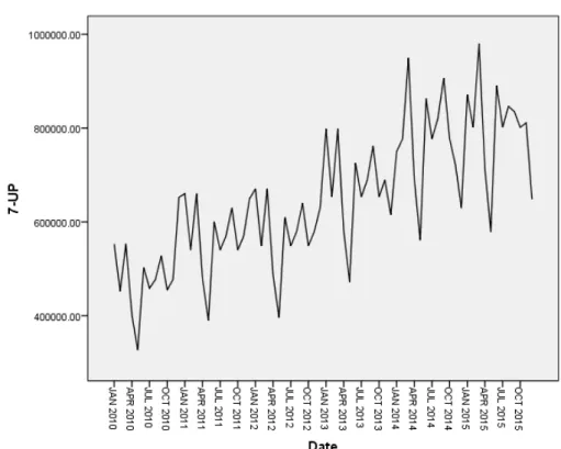
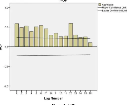
Since the data is a monthly production and utilization, Fig. 1, shows that there is a seasonal cycle of the series and the series is not stationary. The ACF and PACF of the original data, as shown in Fig. 3 and 4, depicts that the sales and utilization data is not stationary. In order to fit an ARIMA model, stationary data in both variance and mean are needed. Stationarity in the variance could be attained by having log transformation and differencing of the original data to attain stationary in the mean. For our data, we need to have seasonal first difference, d = 1, of the original data in order to have stationary series. After that, we need to test the ACF and PACF for the differenced series to check stationary.
Sequence Plot
Table 1: Case Processing Summary
7-UP
Series or Sequence Length 72
Number of Missing Values in the Plot
User-Missing 0
Figure 1: Time plot for sales before differencing
The plot shows the variability of the series appears to be changing with time. Therefore the mean and varianceare not constant, suggesting that the series is not stationary
Time Series Modeler
Table 2: Model Description
Model Type Model ID 7-UP Model_1 ARIMA(0,0,1)(0,1,0)
Model Summary
Table 3: Model Fit
Fit Statistic Mean SE Minimum Maximum
Stationary R-squared .288 . .288 .288 R-squared .880 . .880 .880 RMSE 46432.922 . 46432.922 46432.922 MAPE 5.500 . 5.500 5.500 MaxAPE 16.048 . 16.048 16.048 MAE 37819.886 . 37819.886 37819.886 MaxAE 120607.663 . 120607.663 120607.663 Normalized BIC 21.628 . 21.628 21.628
Table 4: Model Statistics
Model Number of Predictors Model Fit statistics Ljung-Box Q(18) Number of Outliers Stationary R-squared Statistics DF Sig. 7-UP-Model_1 0 .288 23.406 17 .136 0
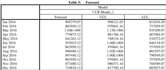
Table 5: Forecast Model 7-UP-Model_1 Forecast UCL LCL Jan 2016 905379.07 998121.65 812636.49 Feb 2016 863950.12 970841.16 757059.07
Mar 2016 1.04E+006 1.15E+006 935209.07
Apr 2016 774875.12 881766.16 667984.07 May 2016 641263.12 748154.16 534372.07 Jun 2016 953025.12 1.06E+006 846134.07 Jul 2016 863950.12 970841.16 757059.07 Aug 2016 908488.12 1.02E+006 801597.07 Sep 2016 897440.12 1.00E+006 790549.07 Oct 2016 863950.12 970841.16 757059.07 Nov 2016 873480.12 980371.16 766589.07 Dec 2016 710818.12 817709.16 603927.07
For each model, forecasts start after the last non-missing in the range of the requested estimation period, and end at the last period for which non-missing values of all the predictors are available or at the end date of the requested forecast period, whichever is earlier.
Figure 2: Numbers Predictor ACF
Table 6: Model Description
Model Name MOD_11
Series Name 1 7-UP
Transformation None
Non-Seasonal Differencing 0
Seasonal Differencing 0
Length of Seasonal Period 12
Maximum Number of Lags 16
Process Assumed for Calculating the Standard Errors of the Autocorrelations Independence(white noise)a
Display and Plot All lags
Applying the model specifications from MOD_11
Table 7: Case Processing Summary
7-UP
Series Length 72
Number of Missing Values User-Missing 0
System-Missing 0
Number of Valid Values 72
Number of Computable First Lags 71
7-UP
Table 8: Autocorrelation
Series: 7-UP
Lag Autocorrelation Std. Errora Box-Ljung Statistic
Value df Sig.b 1 .588 .115 25.920 1 .000 2 .490 .115 44.193 2 .000 3 .528 .114 65.695 3 .000 4 .387 .113 77.415 4 .000 5 .506 .112 97.773 5 .000 6 .538 .111 121.129 6 .000 7 .455 .110 138.130 7 .000 8 .296 .110 145.409 8 .000 9 .345 .109 155.495 9 .000 10 .256 .108 161.116 10 .000 11 .275 .107 167.702 11 .000 12 .595 .106 199.153 12 .000 13 .298 .105 207.188 13 .000 14 .234 .104 212.202 14 .000 15 .252 .103 218.126 15 .000 16 .104 .103 219.154 16 .000
a. The underlying process assumed is independence (white noise). b. Based on the asymptotic chi-square approximation.
Table 9: Partial Autocorrelations
Series: 7-UP
Lag Partial Autocorrelation Std. Error
1 .588 .118 2 .221 .118 3 .279 .118 4 -.056 .118 5 .314 .118 6 .160 .118 7 .061 .118 8 -.314 .118 9 .145 .118 10 -.187 .118 11 .144 .118 12 .496 .118 13 -.380 .118 14 -.040 .118 15 -.150 .118 16 .001 .118
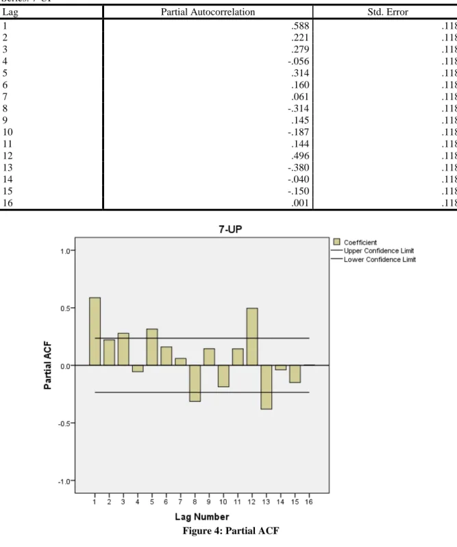
Figure 4: Partial ACF
4.2 Discussion
Since the time plot, autocorrelation and partial autocorrelation functions indicated seasonality in the series, the Autoregressive Integrated Moving Average (ARIMA) model is appropriate. The results are as shown in the Tables 3 to 5. The forecast values for 12 months (Jan. 2016 to Dec. 2016) were shown in Table 5. The Autocorrelation function (ACF) before differencing shows that it has no cyclical pattern but observed that the highest spike is in lag 12. While the Partial Autocorrelation function (PACF) shows that it has a cyclical pattern and cut off after lag 1 but the highest spike is in lag 1, after lag 12 everything tends to zero.
Time plot for quarterly sales as presented in figure 2, after first differencing shows the mean and variance appeared to be constant. Therefore, the series is stationary since the mean and variance are constant. ACF shows there is no correlation function after the first differencing. Therefore the series is stationary. The PACF shows that there is no correlation in the series after first difference. However the series indicate the
presence of AR and MA process models. It is clear that in both the Sales and Utilization that the pattern continues for the upcoming years 2016 and beyond and there are no indications that the quantity sold of Seven-Up products decreases with time.
5. Conclusion
The study aimed at predicting the amount of sales revenue that Seven-Up Bottling Company PLC would realise from January 2016 to December 2016 given the available monthly data on sales revenue from January 2010 to December 2015. This is with a view to find whether there would be an increase or decrease in sales revenue of 7Up Bottling Company’s products. Time plot analysis was used in this research work to analyze the pattern of Sales revenue within the time under study. The study observed that the series have irregular pattern, after taken the first differencing the series became stationary. Nevertheless in modeling ARIMA (p, d, q) the best model is ARIMA (1, 1, 1) for production and ARIMA (0, 1, 1) for utilization. A 12 months forecast have also been made to determine the expected amount of sales revenue in year 2016. The time plot reveals seasonal variation.
ARIMA is a trendy method to analyze stationary univariate time series data. There are generally three main stages to build an ARIMA model, with model identification, model estimation and model checking, of which model classification is the most crucial stage in building ARIMA models. Thus the survey provides an insight into the various time series prediction and forecasting models with reference to ARIMA. Also a lot of real world applications conducted by the various persons were studied and it has come to prove that ARIMA is a real world toll for time series prediction, forecasting and analysis with accuracy.
From the result, the trend used to determine whether sales revenue is increasing or decreasing shows that there is increase in sales revenue of Company with time. From the forecast for sales it shows that Company’s sales revenue will be increasing by each quarter Hence these models can be adopted for sales, production, utilization and demand forecasting in Nigeria.
References
Box, G. E. P. and Tiao, G. C. (1975), “Intervention Analysis with Applications to Economic and Environmental Problems,”Journal of the American Statistical Association, 70, 70–79.
Box, G.E.P. and Jenkins, G.M. (1976). Time Series Analysis: Forecasting and Control. Revised Edn. (Hoden-Day, San Francisco, 1976). http://adsabs.harvard.edu/abs/1976tsaf.conf...B
Chatfild, C. (1996). The Analysis of Time Series-an introduction, 5th Edition (Chapman and Hall, UK.) Hanke, J. E. & Wichern, D. W., 2005. Business forecasting. 8th ed. Upper Saddle River: Rearson.
Lapide, L., (2009). History to demand-driven forecasting. The Journal of Business, 2(28), 18-19.
Makridakis, S., Wellwright, S. C. and Hyndman, R. J. (1998). Forecasting Methods and Applications. 3rd Edition. John Wiley, U.S.A
Makridakis, S. & Hibon, M., 2000. The M3-Competition: results, conclusions and implications. International Journal of Forecasting, 16(4), p. 451–476.
Montgomery, D.C. and Johnson, L.A. (1967). Forecasting and Time Series Analysis.(McGrow-Hill Book Company), http://www.abebooks.com/Forecasting-Time-
Pankratz, A. (1991), Forecasting with Dynamic Regression Models, New York: John Wiley & Sons.
Pant, N. P. & Starbuck, W. H., 1990. Innocents in the Forest: Forecasting and ResearchMethods. Journal of Management, 16(2), pp. 433-460.