Hierarchical ensemble methods for protein function prediction

Review Article

Hierarchical Ensemble Methods for Protein Function Prediction

Giorgio Valentini

AnacletoLab-Dipartimento di Informatica, Universit`a degli Studi di Milano, Via Comelico 39, 20135 Milano, Italy Correspondence should be addressed to Giorgio Valentini; [email protected]

Received 2 February 2014; Accepted 25 February 2014; Published 5 May 2014 Academic Editors: T. Can and T. R. Hvidsten

Copyright © 2014 Giorgio Valentini. This is an open access article distributed under the Creative Commons Attribution License, which permits unrestricted use, distribution, and reproduction in any medium, provided the original work is properly cited. Protein function prediction is a complex multiclass multilabel classification problem, characterized by multiple issues such as the incompleteness of the available annotations, the integration of multiple sources of high dimensional biomolecular data, the unbalance of several functional classes, and the difficulty of univocally determining negative examples. Moreover, the hierarchical relationships between functional classes that characterize both the Gene Ontology and FunCat taxonomies motivate the development of hierarchy-aware prediction methods that showed significantly better performances than hierarchical-unaware “flat” prediction methods. In this paper, we provide a comprehensive review of hierarchical methods for protein function prediction based on ensembles of learning machines. According to this general approach, a separate learning machine is trained to learn a specific functional term and then the resulting predictions are assembled in a “consensus” ensemble decision, taking into account the hierarchical relationships between classes. The main hierarchical ensemble methods proposed in the literature are discussed in the context of existing computational methods for protein function prediction, highlighting their characteristics, advantages, and limitations. Open problems of this exciting research area of computational biology are finally considered, outlining novel perspectives for future research.

1. Introduction

Exploiting the wealth of biomolecular data accumulated by novel high-throughput biotechnologies, “in silico” protein function prediction can generate hypotheses to drive the

bio-logical discovery and validation of protein functions [1].

Indeed, “in vitro” methods are costly in time and money, and automatic prediction methods can support the biologist in understanding the role of a protein or of a biological process or in annotating a new genome at high level of accuracy or more, in general, in solving problems of functional genomics

[2].

TheAutomated Function Prediction(AFP) is a multiclass, multilabel classification problem characterized by hundreds or thousands of functional classes structured according to a predefined hierarchy. Even in principle, also unsupervised methods can be applied to AFP, due to the inherent difficulty of extracting functional classes without exploiting any

avail-able a priori information [3,4]; usually supervised or

semi-supervised learning methods are applied in order to exploit the available a priori information about gene annotations.

From a computational standpoint, AFP is a challenging problem for several reasons.

(i)The number of functional classes is usually large:

hundreds for the Functional Catalogue (FunCat) [5]

or thousands for the Gene Ontology (GO) [6].

(ii)Proteins may be annotated for multiple functional classes: since each protein may belong to more than one class at the same time, the classification problem is multilabel.

(iii)Multiple sources of data are available for each protein:

high-throughput biotechnologies make an increas-ing number of sources of genomic and proteomic data available. Hence, in order to exploit all the information available for each protein, we need to learn methods that are able to integrate different data

sources [7].

(iv)Functional classes are hierarchically related: annota-tions are not independent because functional classes are hierarchically organized; in general, known func-tional relationships (such as taxonomies) can be exploited to incorporate a priori knowledge in learn-ing algorithms or to introduce explicit constraints between labels.

Volume 2014, Article ID 901419, 34 pages http://dx.doi.org/10.1155/2014/901419

(v)Small number of annotations for each class: typically, functional classes are severely unbalanced, with a small number of available “positive” annotations. (vi)Multiple possible definitions of negative examples:

since we only have positive annotations (the total

number of GO negative annotations is about2500,

considering all species (August 2013)), the notion of negative example is not uniquely determined, and different strategies of choosing negative examples can

be applied in principle [8].

(vii)Different reliability of functional labels: functional

annotations have different degrees of evidence; that is, each label is assigned to a gene with a specific level of reliability.

(viii)Complex and noisy data: data are usually complex

(e.g., high-dimensional, large-scale, and graph-stru-ctured) and noisy.

Most of the computational methods for AFP have been

applied to unicellular organisms (e.g.,S. cerevisiae) [9–11], but

recently several approaches have been applied to multicellular

organisms (such as M. musculus or the A. thaliana plant

model organisms [2,12–16]).

Several computational approaches, and in particular machine learning methods, have been proposed to deal with

the above issues, ranging from sequence-based methods [17]

to network-based methods [18], structured output algorithm

based on kernels [19], and hierarchical ensemble methods

[20].

Other approaches focused primarily on the integration of multiple sources of data, since each type of genomic data captures only some aspects of the genes to be classified, and a specific source can be useful to learn a specific functional class while being irrelevant to others. In the literature, many approaches have been proposed to deal with this topic,

for example, functional linkage networks integration [21],

kernel fusion [11], vector space integration [22], and ensemble

systems [23].

Extensive experimental studies showed that flat predic-tion, that is, predictions for each class made independently of the other classes, introduces significant inconsistencies

in the classification, due to the violation of the true path

rulethat governs the functional annotations of genes both

in the GO and in FunCat taxonomies [24]. According to

this rule, positive predictions for a given term must be transferred to its “ancestor” terms and negative predictions

to its descendants (seeAppendix Aand Section 7for more

details about the GO and the true path rule). Moreover flat predictions are difficult to interpret because they may be inconsistent with one another. A method that claims, for example, that a protein has homodimerization activity but does not have dimerization activity is clearly incorrect, and a biologist attempting to interpret these results would not likely

trust either prediction [24].

It is worth noting that the results of the Critical Assessment of Functional Annotation (CAFA) challenge, a recent comprehensive critical assessment and comparison

of different computational methods for AFP [16], showed

that AFP is characterized by multiple complex issues, and one of the best performing CAFA methods corrected flat predictions taking into account the hierarchical relationships between functional terms, with an approach similar to that

adopted by hierarchical ensemble methods [25]. Indeed,

hier-archical ensemble methods embed in the learning process the relationships between functional classes. Usually, this is performed in a second “reconciliation” step, where the predictions are modified to make them consistent with the

ontology [26–29]. More, in general, these methods exploit the

relationships between ontology terms, structured according

to a forest of trees [5] or a directed acyclic graph [6] to

significantly improve prediction performances with respect

to “flat” prediction methods [30–32].

Hierarchical classification and in particular ensemble methods for hierarchical classification have been applied in several domains different from protein function prediction,

ranging from text categorization [33–35] to music genre

classification [36–38], hierarchical image classification [39,

40] and video annotation [41], and automatic classification

of worldwide web documents [42, 43]. The present review

focuses on hierarchical ensemble methods for AFP. For a more general review on hierarchical classification methods

and their applications in different domains, see [44].

The paper is structured as follows. In Section 2, we

provide a synthetic picture of the main categories of protein function methods, to properly position hierarchical ensemble methods in the context of computational methods for AFP. In

Section 3, the main common characteristics of hierarchical ensemble algorithms, as well as a general taxonomy of these methods, are proposed. The following five sections focus on the main families of hierarchical methods for AFP

and discuss their main characteristics.Section 4introduces

hierarchical top-down methods,Section 5Bayesian ensemble

approaches,Section 6reconciliation methods,Section 7true

path rule ensemble methods, and the last one (Section 8)

ensembles based on decision trees. Section 9critically

dis-cusses the main issues and limitations of hierarchical ensem-ble methods and shows that this approach, such as the other current approaches for AFP, cannot be successfully applied without considering the large set of complex learning issues that characterize the AFP problem. The last two sections discuss the open problems and future possible research lines in the context of hierarchical ensemble methods and summarize the main findings in this exciting research area. In the Appendix, some basic information about the FunCat and the GO, that is, the two main hierarchical ontologies that are widely used to annotate proteins in all organisms, are provided, as well as the characteristics of the hierarchical-aware performance measures proposed in the literature to assess the accuracy and the reliability of the predictions made by hierarchical computational methods.

2. A Taxonomy of Protein Function

Prediction Methods

Several computational methods for the AFP problem have been proposed in the literature. Some methods provided predictions of a relatively small set of functional classes

[11,45,46], while others considered predictions extended to larger sets, using support vector machines and semidefinite

programming [11], artificial neural networks [47], functional

linkage networks [21,48], Bayesian networks [45], or

meth-ods that combine functional linkage networks with learning

machines using a logistic regression model [12] or simple

algebraic operators [13].

Other research lines for AFP explicitly take into account the hierarchical nature of the multilabel classification prob-lem. For instance, structured output methods are based on the joint kernelization of both input variables and output labels,

using, for example, perceptron-like learning algorithms [49]

or maximum-margin algorithms [50]. Other approaches

improve the prediction of GO annotations by extracting implicit semantic relationships between genes and functions

[51]. Finally, other methods adopted an ensemble approach

[52] to take advantage of the intrinsic hierarchical nature

of protein function prediction, explicitly considering the

relationships between functional classes [24,53–55].

Computational methods for AFP, mostly based on machine learning methods, can be schematically grouped in the following four families:

(1) sequence-based methods; (2) network-based methods;

(3) kernel methods for structured output spaces; (4) hierarchical ensemble methods.

This grouping is neither exhaustive nor strict, meaning that certain methods do not belong to any of these groups, and others belong to more than one.

2.1. Sequence-Based Methods. Algorithms based on align-ment of sequences represent the first attempts to

compu-tationally predict the function of proteins [56, 57]: similar

sequences are likely to share common functions, even if it is well known that secondary and tertiary structure con-servation are usually more strictly related to protein func-tions. However, algorithms able to infer similarities between sequences are today standard methods of assigning functions

to proteins in newly sequenced organisms [17,58]. Of course,

global or local structure comparison algorithms between

proteins can be applied to detect functional properties [59],

and, in this context, the integration of different sequence and structure-based prediction methods represents a major

challenge [60].

Even if most of the research efforts for the design and development of AFP methods concentrated on machine learning methods, it is worth noting that in the AFP 2011

challenge [16] one of the best performing methods is

repre-sented by a sequence-based algorithm [61]. Indeed, when the

only information available is represented by a raw sequence of amino acids or nucleotides, sequence-based methods can be competitive with state-of-the-art machine learning methods

by exploiting homology-based inference [62].

2.2. Network-Based Methods. These methods usually

repre-sent each dataset through an undirected graph𝐺 = (𝑉, 𝐸),

where nodesV ∈ 𝑉correspond to gene/gene products and

edges 𝑒 ∈ 𝐸 are weighted according to the evidence of

cofunctionality implied by data source [63,64]. These

algo-rithms are able to transfer annotations from previously annotated (labeled) nodes to unannotated (unlabeled) ones by exploiting “proximity relationships” between connected nodes. Basically, these methods are based on transductive label propagation algorithms that predict the labels of unan-notated examples without using a global predictive model

[14,21,45]. Several method exploited the semantic similarity

between GO terms [65, 66] to derive functional similarity

measures between genes to construct functional terms, using then supervised or semisupervised learning algorithm to

infer GO annotations of genes [67–70].

Different strategies to learn the unlabeled nodes have been explored by “label propagation” algorithms, that is, methods able to “propagate” the labels of annotated proteins across the networks, by exploiting the topology of the under-lying graph. For instance, methods based on the evaluation

of the functional flow in graphs [64,71], methods based on

the Hopfield networks [48, 72, 73], methods based on the

Markov [74,75] and Gaussian random fields [14,46], and also

simple “guilt-by-association” methods [76,77], based on the

assumption that connected nodes/proteins in the functional networks are likely to share the same functions. Recently, methods based on kernelized score functions, able to exploit both local and global semisupervised learning strategies, have

been successfully applied to AFP [78] as well as to disease

gene prioritization [79] and drug repositioning problems

[80,81].

Reference [82] showed that different graph-based

algo-rithms can be cast into a common framework where a quadratic cost objective function is minimized. In this frame-work, closed form solutions can be derived by solving a linear system of size equal to the cardinality of nodes (proteins) or

using fast iterative procedures such as the Jacobi method [83].

A network-based approach, alternative to label propagation and exhibiting strong theoretical predictive guarantees in the so-called mistake bound model, has been recently proposed

by [84].

2.3. Kernel Methods for Structured Output Spaces. By extend-ing kernels to the output space, the multilabel hierarchical classification problem is solved globally: the multilabels are viewed as elements of a structured space modeled by suitable

kernel functions [85–87], and structured predictions are

viewed as a maximum a posteriori prediction problem [88].

Given a feature spaceXand a space of structured labels

Y, the task is to learn a mapping𝑓 :X → Yby an induced

joint kernel function𝑘that computes the “compatibility” of

a given input-output pair(𝑥, 𝑦): for each test example𝑥 ∈

X, we need to determine the label𝑦 ∈ Ysuch that 𝑦 =

arg max_𝑦∈Y𝑘(𝑥, 𝑦), for any𝑥 ∈X. By modeling probabilities

by a log-linear model, and using a suitable feature map

𝜙(𝑥, 𝑦), we can define an induced joint kernel function that uses both inputs and outputs to compute the “compatibility”

of a given input-output pair [88]

Structured output methods infer a label ̂𝑦 by finding the

maximum of a function𝑔that uses the previously defined

joint kernel (1)

̂𝑦 =arg max

𝑦∈Y𝑔 (𝑥, 𝑦) . (2)

TheGOstructsystem implemented a structured percep-tron and a variant of the structured support vector machine

[85]. This approach has been successfully applied to the

prediction of GO terms in mouse and other model organisms

[19]. Structured output maximum-margin algorithms have

been also applied to the tree-structured prediction of enzyme

functions [50,86].

2.4. Hierarchical Ensemble Methods. Other approaches take explicitly into account the hierarchical relationships between

functional terms [26,29,53,54,89,90]. Usually, they modify

the “flat” predictions (i.e., predictions made independently of the hierarchical structure of the classes) and correct them improving accuracy and consistency of the multilabel

annotations of proteins [24].

The flat approach makes predictions for each term inde-pendently and, consequently, the predictor may assign to a single protein a set of terms that are inconsistent with one another. A possible solution for this problem is to train a classifier for each term of the reference ontology to produce a set of prediction at each term and, finally, to reconcile the predictions by taking into account the relationships between the classes of the ontology. Different ensemble based algorithms have been proposed ranging from methods

restricted to multilabels with single and no partial paths [91]

to methods extended to multiple and also partial paths [92].

Many recent published works clearly demonstrated that this approach ensures an increment in precision, but this comes

at expenses of the overall recall [2,30].

In the next section, we discuss in detail hierarchical ensemble methods, since they constitute the main topic of this review.

3. Hierarchical Ensemble Methods:

Exploiting the Hierarchy to

Improve Protein Function Prediction

Ensemble methods are one of the main research areas of

machine learning [52, 93–95]. From a general standpoint,

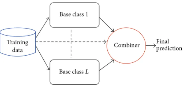
ensembles of classifiers are sets of learning machines that

work together to solve a classification problem (Figure 1).

Empirical studies showed that in both classification and regression problems ensembles improve on single learning machines, and, moreover, large experimental studies com-pared the effectiveness of different ensemble methods on

benchmark data sets [96–99], and they have been successfully

applied to several computational biology problems [100–104].

Ensemble methods have been also successfully applied in an

unsupervised setting [105, 106]. Several theories have been

proposed to explain the characteristics and the successful application of ensembles to different application domains. For instance, Allwein, Schapire, and Singer interpreted the

Training data Combiner Final prediction Base class1 Base classL

Figure 1: Ensemble of classifiers.

improved generalization capabilities of ensembles of learning

machines in the framework of large margin classifiers [107,

108]; Kleinberg, in the context of Stochastic Discrimination

Theory [109], and Breiman and Friedman in the light of

the bias-variance analysis borrowed from classical statistics

[110,111]. The interest in this research area is motivated also by

the availability of very fast computers and networks of work-stations at a relatively low cost that allow the implementation and the experimentation of complex ensemble methods using off-the-shelf computer platforms.

Constraints between labels and, more in general, the issue of label dependence have been recognized to play a

central role in multilabel learning [112]. Protein function

prediction can be regarded as a paradigmatic multilabel classification problem, where the exploitation of a priori knowledge about the hierarchical relationships between the labels can dramatically improve classification performance

[24,27,113].

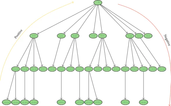
In the context of AFP problems, ensemble methods reflect the hierarchy of functional terms in the structure of the ensemble itself: each base learner is associated with a node of the graph representing the functional hierarchy and learns a specific GO term or FunCat category. The predictions provided by the trained classifiers are then combined by exploiting the hierarchical relationships of the taxonomy.

In their more general form, hierarchical ensemble meth-ods adopt a two-step learning strategy.

(1) In the first step, each base learner separately or inter-acting with connected base learners learns the protein functional category on a per term basis. In most cases, this yields a set of independent classification prob-lems, where each base learning machine is trained to learn a specific functional term, independently of the other base learners.

(2) In the second step, the predictions provided by the trained classifiers are combined by considering the hierarchical relationships between the base classifiers modeled according to the hierarchy of the functional classes.

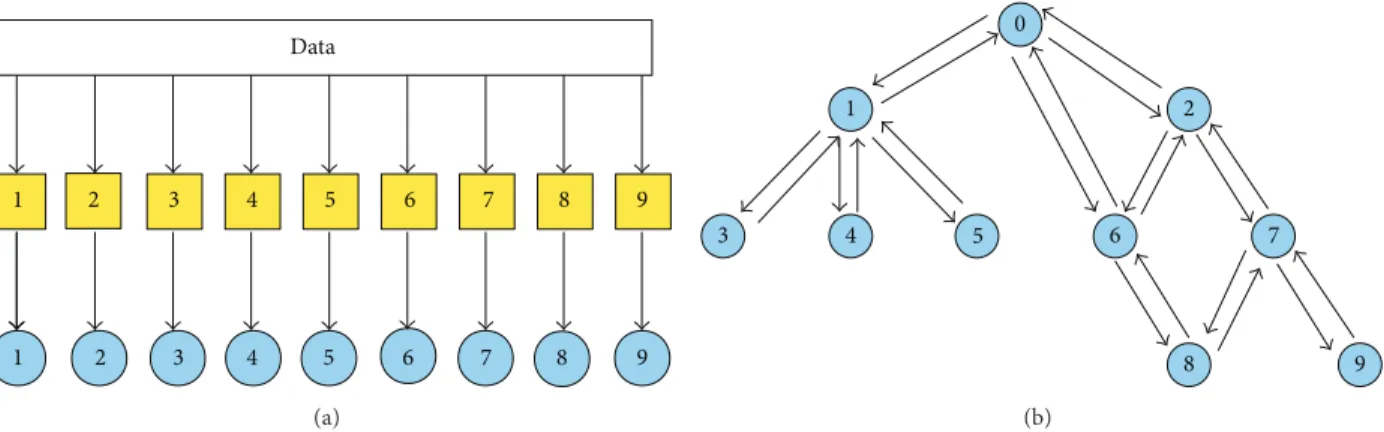
Figure 2 depicts the two learning steps of hierarchical ensemble methods. In the first step, a learning algorithm

(a square object in Figure 2(a)) is applied to train the

base classifiers associated with each class (represented with

1 2 3 4 5 6 7 8 9 1 2 3 4 5 6 7 8 9 Data (a) 0 1 2 3 4 5 6 7 8 9 (b)

Figure 2: Schematic representation of the two main learning steps of hierarchical ensemble methods. (a) Training of base classifiers; (b) top-down and/or bottom-up propagation of the predictions.

(circles) in the prediction phase exploit the hierarchical relationships between classes to combine its predictions with

those provided by the other base classifiers (Figure 2(b)).

Note that the dummy 0node is added to obtain a rooted

hierarchy. Up and down arrows represent the possibility of combining predictions by exploiting those provided, respec-tively, by children and parents classifiers, according to a bottom-up or top-down learning strategy. Note that both “local” combinations are possible (e.g., the prediction of

node5may depend only on the prediction of node1), but

also “global” combinations can be considered, by taking into account the predictions across the overall structure of the

graph (e.g., predictions for node 9 can depend on all the

predictions made by all the other base classifiers from1to

8). Moreover, both top-down propagation of the predictions

(down arrows,Figure 2(b)) and bottom-up propagation (up

arrows) can be considered, depending on the specific design of the hierarchical ensemble algorithm.

This ensemble approach is highly modular: in principle, any learning algorithm can be used to train the classifiers in the first step, and both annotation decisions, probabilities, or whatever scores provided by each base learner can be combined, depending on the characteristics of the specific hierarchical ensemble method.

In this section, we provide some basic notations and an ensemble taxonomy that will be used to introduce the different hierarchical ensemble methods for AFP.

3.1. Basic Notation. A gene/gene product𝑔 can be

repre-sented through a vectorx ∈ R𝑑 having𝑑different features

(e.g., gene expression levels across 𝑑 different conditions,

sequence similarities with other genes/proteins, or presence or absence of a given domain in the corresponding protein or genetic or physical interaction with other proteins). Note that we, for the sake of simplicity and with a certain approxi-mation, refer in the same way to genes and proteins, even if it is well known that a given gene may correspond to multiple

proteins. A gene𝑔 is assigned to one or more functional

classes in the set𝐶 = {𝑐₁, 𝑐₂, . . . , 𝑐_𝑚}structured according to

a FunCat forest of trees𝑇or a directed acyclic graph 𝐺of

the Gene Ontology (usually a dummy root class𝑐₀, which

every gene belongs to, is added to 𝑇or𝐺 to facilitate the

processing). The assignments are coded through a vector of

multilabelsy= (𝑦₁, 𝑦₂, . . . , 𝑦_𝑚) ∈ {0, 1}𝑚, where𝑔belongs to

class𝑐_𝑖if and only if𝑦_𝑖= 1.

In both the Gene Ontology(GO) and FunCat taxonomies, the functional classes are structured according to a hierarchy and can be represented by a directed graph, where nodes correspond to classes and edges correspond to relationships between classes. Hence, the node corresponding to the class

𝑐_𝑖can be simply denoted by𝑖. We represent the set of children

nodes of 𝑖by child(𝑖), and the set of its parents by par(𝑖).

Moreover,𝑦child(𝑖) denotes the labels of the children classes

of node 𝑖 and analogously𝑦par(𝑖) denotes the labels of the

parent classes of𝑖. Note that in FunCat only one parent is

permitted, since the overall hierarchy is a tree forest, while, in the GO, more parents are allowed, because the relationships are structured according to a directed acyclic graph.

Hierarchical ensemble methods train a set of calibrated

classifiers, one for each node of the taxonomy𝑇. These

clas-sifiers are used to derive estimates ̂𝑝_𝑖(𝑔)of the probabilities

𝑝_𝑖(𝑔) = P(𝑉_𝑖 = 1 | 𝑉par(𝑖) = 1, 𝑔)for all𝑔and𝑖, where

(𝑉₁, . . . , 𝑉_𝑚) ∈ {0, 1}𝑚_{is the vector random variable modeling}

the unknown multilabel of a gene𝑔, and𝑉par(𝑖) denotes the

random variables associated with the parents of node𝑖. Note

that𝑝_𝑖(𝑔)are probabilities conditioned to𝑉par(𝑖) = 1, that

is, the probability that a gene is annotated to a given term

𝑖, given that the gene is just annotated to its parent terms,

thus respecting the true path rule. Ensemble methods infer

a multilabel assignment̂y = ( ̂𝑦₁, . . . , ̂𝑦_𝑚) ∈ {0, 1}𝑚based on

estimates ̂𝑝₁(𝑔), . . . , ̂𝑝_𝑚(𝑔).

3.2. A Taxonomy of Hierarchical Ensemble Methods. Hierar-chical ensemble methods for AFP share several character-istics, from the two-step learning approach to the exploita-tion of the hierarchical relaexploita-tionships between classes. For these reasons, it is quite difficult to clearly and univocally individuate taxonomy of hierarchical ensemble methods. Here, we show taxonomy useful mainly to describe and discuss existing methods for AFP. For a recent review and taxonomy of hierarchical ensemble methods, not specific for

AFP problems, we refer the reader to the comprehensive Silla

and others’ review [44].

In the following sections, we discuss the following groups of hierarchical ensemble methods:

(i) top-down ensemble methods. These methods are characterized by a simple top-down approach in the second step: only the output of the parent node/base classifier influences the output of the children, thus resulting in a top-down propagation of the decisions; (ii) Bayesian ensemble methods. These are a class of methods theoretically well founded and in some cases they are optimal from a Bayesian standpoint; (iii) Reconciliation methods. This is a heterogeneous class

of heuristics by which we can combine the predictions of the base learners, by adopting different “local” or “global” combination strategies;

(iv) true path rule ensembles. These methods adopt a heuristic approach based on the “true path rule” that governs both the GO and FunCat ontologies; (v) decision tree-based ensembles. These methods are

characterized by the application of decision trees as base learners or by adopting decision tree-like learning strategies to combine predictions of the base learners.

Despite this general characterization, several methods could be assigned to different groups, and for several hierar-chical ensemble methods it is difficult to assign them to any the introduced classes of methods.

For instance, in [114–116] the authors used the hierarchy

only to construct training sets different for each term of the Gene Ontology, by determining positive and negative examples on the basis of the relationships between functional

terms. In [89] for each classifier associated with a node, a gene

is labeled as positive (i.e., belonging to the term associated with that node) if it actually belongs to that node or as negative if it does not belong to that node or to the ancestors or descendants of the node.

Other approaches exploited the correlation between

nearby classes [32,53,117]. Shahbaba and Neal [53] take into

account the hierarchy to introduce correlation between func-tional classes, using a multinomial logit model with Bayesian

priors in the context of E. coli functional classification

with Riley’s hierarchies [118]. Bogdanov and Singh

incorpo-rated functional interrelationships between terms during the extraction of features based on annotations of neighboring genes and then applied a nearest-neighbor classifier to predict

protein functions [117]. The HiBLADE method (hierarchical

multilabel boosting with label dependency) [32] not only

takes advantage of the preestablished hierarchical taxonomy of the classes but also effectively exploits the hidden corre-lation among the classes that is not shown through the class hierarchy, thereby improving the quality of the predictions. In particular, the dependencies of the children for each label in the hierarchy are captured and analyzed using the Bayes method and instance-based similarity. Experiments using the FunCat taxonomy and the yeast model organism

show that the proposed method is competitive with TPR-W (Section 7.2) and HABYES-CS (Section 5.3) hierarchical ensemble methods.

An adaptation of a classical multiclass boosting algorithm

[119] has been adapted to fit the hierarchical structure of the

FunCat taxonomy [120]: the method is relatively simple and

straightforward to be implemented and achieves competitive results for the AFP in the yeast model organism.

Finally, other hierarchical approaches have been pro-posed in the context of competitive networks learning frame-work. Competitive networks are well-known unsupervised and supervised methods able to map the input space into a structured output space where clusters or classes are usually arranged according to a grid topology and where learning adopts at the same way a competition, cooperation, and

adaptation strategy [121]. Interestingly enough, in [122], the

authors adopted this approach to predict the hierarchy of gene annotations in the yeast model organism, by using a tree-topology according to the FunCat taxonomy: each neuron is connected with its parent or with its children. Moreover, each neuron in tree-structured output layer is connected to all neurons of the input layer, representing the instances, that is, the set of genomic features associated with each gene to be classified. Results obtained with the hierarchy of enzyme commission codes showed that this approach is competitive with those obtained with hierarchical decision

trees ensembles [29] (Section 8).

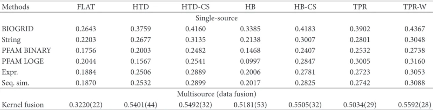
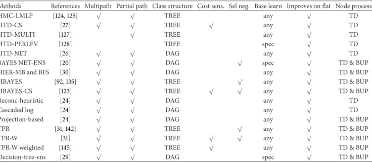
To provide a general picture of the methods discussed

in the following sections, Table 1 summarizes their main

characteristics. The first two columns report the name and a reference to the method, the third whether multiple or single paths across the taxonomy are allowed, and the next whether partial paths are considered (i.e., paths that do not end with a leaf). The successive columns refer to the class structure (a tree or a DAG), to the adoption or not of cost-sensitive (i.e., unbalance-aware) classification approaches, and to the adoption of strategies to properly select negative examples in the training phase. Finally, the last three columns summarize the type of the base learner used (“spec” means that only a specific type of base learner is allowed and “any” means that any type of learner can be used within the method), whether the method improves or not with respect to the flat approach, and the mode of processing of the nodes (“TD”: down approach, and “TD&BUP”: adopting both top-down and bottom-up strategies). Of course methods having more checkmarks are more flexible and in general methods that can process a DAG can also process tree-structured ontologies, but the opposite is not guaranteed, while the type of node processing relies on the way the information is propagated across the ontology. It is worth noting that all the considered methods improve on baseline “flat” classification methods.

4. Hierarchical Top-Down (HTD) Ensembles

These ensemble methods exploit the hierarchical relation-ships between functional terms in a top-to-bottom fashion, that is, considering only the relationships denoted by the

Table 1: Characteristics of some of the main hierarchical ensemble methods for AFP.

Methods References Multipath Partial path Class structure Cost sens. Sel neg. Base learn Improves on flat Node process

HMC-LMLP [124,125] √ √ TREE any √ TD

HTD-CS [27] √ √ TREE √ any √ TD

HTD-MULTI [127] √ TREE any √ TD

HTD-PERLEV [128] TREE spec √ TD

HTD-NET [26] √ √ DAG any √ TD

BAYES NET-ENS [20] √ √ DAG √ spec √ TD & BUP

HIER-MB and BFS [30] √ √ DAG any √ TD & BUP

HBAYES [92,135] √ √ TREE √ any √ TD & BUP

HBAYES-CS [123] √ √ TREE √ √ any √ TD & BUP

Reconc-heuristic [24] √ √ DAG any √ TD

Cascaded log [24] √ √ DAG any √ TD

Projection-based [24] √ √ DAG any √ TD & BUP

TPR [31,142] √ √ TREE √ any √ TD & BUP

TPR-W [31] √ √ TREE √ √ any √ TD & BUP

TPR-W weighted [145] √ √ TREE √ any √ TD & BUP

Decision-tree-ens [29] √ √ DAG spec √ TD & BUP

ensemble method (HTD) algorithm is straightforward: for

each gene𝑔, starting from the set of nodes at the first level

of the graph𝐺(denoted by root(𝐺)), the classifier associated

with the node𝑖 ∈ 𝐺computes whether the gene belongs to the

class𝑐_𝑖. If yes, the classification process continues recursively

on the nodes𝑗 ∈ child(𝑖); otherwise, it stops at node𝑖, and

the nodes belonging to the descendants rooted at𝑖are all set

to0. To introduce the method, we use probabilistic classifiers

as base learners trained to predict class𝑐_𝑖associated with the

node𝑖of the hierarchical taxonomy. Their estimates ̂𝑝_𝑖(𝑔)of

P(𝑉_𝑖 = 1 | 𝑉par(𝑖) = 1, 𝑔)are used by the HTD ensemble to

classify a gene𝑔as follows:

̂𝑦𝑖= { { { { { { { { { { { { ̂𝑝𝑖(𝑔) >1₂} if𝑖 ∈root(𝐺) { ̂𝑝_𝑖(𝑔) >1₂} if𝑖 ∉root(𝐺) ∧ { ̂𝑝par(𝑖)(𝑔) > 1₂} 0 if𝑖 ∉root(𝐺) ∧ { ̂𝑝par(𝑖)(𝑔) ≤ 1₂} , (3)

where {𝑥} = 1 if 𝑥 > 0; otherwise, {𝑥} = 0 and

̂𝑝par(𝑖) is the probability predicted for the parent of the term

𝑖. It is easy to see that this procedure ensures that the

predicted multilabelŝy = ( ̂𝑦₁, . . . , ̂𝑦_𝑚)are consistent with

the hierarchy. We can apply the same top-down procedure also using nonprobabilistic classifiers, that is, base learners generating continuous scores, or also discrete decisions, by

slightly modifying (3).

In [123], a cost-sensitive version of the basic top-down

hierarchical ensemble method HTD has been proposed: by

assigninĝ𝑦_𝑖before the label of any𝑗in the subtree rooted at

𝑖, the following rule is used:

̂𝑦𝑖= { ̂𝑝𝑖≥ 1₂} × { ̂𝑦par(𝑖)= 1} (4) for𝑖 = 1, . . . , 𝑚(note that the guessed label ̂𝑦₀ of the root

of𝐺is always1). Then, the cost-sensitive variant HTD-CS

introduces a single cost-sensitive parameter 𝜏 > 0 which

replaces the threshold1/2. The resulting rule for HTD-CS is

then

̂𝑦𝑖= { ̂𝑝𝑖≥ 𝜏} × { ̂𝑦par(𝑖)= 1} . (5)

By tuning𝜏, we may obtain ensembles with different

pre-cision/recall characteristics. Despite the simplicity of the hierarchical top-down methods, several works showed their

effectiveness for AFP problems [28,31].

For instance, Cerri and De Carvalho experimented differ-ent variants of top-down hierarchical ensemble methods for

AFP [28,124,125]. The HMC-LMLP (hierarchical multilabel

classification with local multilayer perceptron) successively trains a local MLP network for each hierarchical level, using

the classical backpropagation algorithm [126]. Then, the

output of the MLP for the first layer is used as input to train the MLP that learns the classes of the second level

and so on (Figure 3). A gene is annotated to a class if its

corresponding output in the MLP is larger than a predefined threshold; then, in a postprocessing phase (second-step of the hierarchical classification), inconsistent predictions are removed (i.e., classes predicted without the prediction of their

superclasses) [125]. In practice, instead of using a dichotomic

classifier for each node, the HMC-LMLP algorithm applies a single multiclass multilayer perceptron for each level of the hierarchy.

A related approach adopts multiclass classifiers (HTD-MULTI) for each node, instead of a simple binary classifier, and tries to find the most likely path from the root to the leaves of the hierarchy, considering simple techniques, such as the multiplication or the sum of the probabilities estimated

at each node along the path [127]. The method has been

applied to the cell cycle branch of the FunCat hierarchy with the yeast model organism, showing improvements with respect to classical hierarchical top-down methods, even if the proposed approach can only predict classes along a single

Input instancex

Layers corresponding to

Layers corresponding to the first hierarchical level

the second hierarchical level

Hidden neurons Hidden neurons

Outputs of the first level (classes) are provided as inputs to the

network of the second level

Outputs of the second level (classes) . . . . . . . . . _. . . . . . . . . . . . . . . . . . . . . . . . x1 x2 x3 x4 xN

Figure 3: HMC-LMLP: outputs of the MLP responsible for the predictions in the first level are used as input to another MLP for the predictions in the second level (adapted from [125]).

“most likely path,” thus not considering that in AFP we may have annotations involving multiple and partial paths.

Another method that introduces multiclass classifiers instead of simple dichotomic classifiers has been proposed by

Paes et al. [128]: local per level multiclass classifiers

(HTD-PERLEV) are trained to distinguish between the classes of a specific level of the hierarchy, and two different strategies to remove inconsistencies are introduced. The method has been applied to the hierarchical classification of enzymes using the EC taxonomy for the hierarchical classification of enzymes, but unfortunately this algorithm is not well suited to AFP, since leaf nodes are mandatory (that is partial path annotations are not allowed) and multilabel annotations along multiple paths are not allowed.

Another interesting top-down hierarchical approach pro-posed by the same authors is HMC-LP (hierarchical multil-abel classification lmultil-abel-powerset), a hierarchical variation of thelabel-powerset nonhierarchical multilabel method [129], that has been applied to the prediction of gene function of the yeast model organism using 10 different data sets and

the FunCat taxonomy [124]. According to thelabel-powerset

approach, the method is based on a first label-combination step by which, for each example (gene), all classes assigned to the example are combined into a new and unique class, and this process is repeated for each level of the hierarchy. In this way, the original problem is transformed into a hierarchical single-label problem. In both the training and test phases, the top-down approach is applied, and at the end of the classification phase the original classes can be

easily reconstructed [124]. In an experimental comparison

using the FunCat taxonomy forS. cerevisiae,results showed

that hierarchical top-down ensemble methods significantly outperform decision trees-based hierarchical methods, but no significant difference between different flavors of

top-down hierarchical ensembles has been detected [28].

Top-down algorithms can be conceived also in the con-text of network-based methods (HTD-NET). For instance, in

[26], a probabilistic model that combines relational

protein-protein interaction data and the hierarchical structure of GO to predict true-path consistent function labels obeys the true path rule by setting the descendants of a node as negative whenever that node is set to negative. More precisely, the authors at first compute a local hierarchical conditional probability, in the sense that, for any nonroot GO term, only the parents affect its labeling. This probability is computed within a network-based framework assuming that the labeling of a gene is independent of any other genes given that of its neighbors (a sort of the Markov property with respect to gene functional interaction networks) and assuming also a binomial distribution for the number of neighbors labeled with child terms with respect to those labeled with the parent term. These assumptions are quite stringent but are necessary to make the model tractable. Then, a global hierarchical conditional probability is computed by recursively applying the previously computed local hierarchi-cal conditional probability by considering all the ancestors.

More precisely, by assuming thatP( ̂𝑦_𝑖= 1 | 𝑔, 𝑁(𝑔)), that is,

the probability that a gene𝑔is annotated for a a node𝑖, given

the status of the annotations of its neighborhood 𝑁(𝑔) in

the functional networks, the global hierarchical conditional probability factorizes according to the GO graph as follows:

P( ̂𝑦𝑖= 1 | 𝑔, 𝑁 (𝑔))

= ∏

𝑗∈anc(𝑖)

P( ̂𝑦_𝑗 = 1 | ̂𝑦par(𝑗)= 1, 𝑁loc(𝑔)) ,

(6)

where𝑁_loc(𝑔)represents the local hierarchical neighborhood

information on the parent-child GO term pair par(𝑗) and

𝑗[26]. This approach guarantees to produce GO term label

assignments consistent with the hierarchy, without the need of a postprocessing step.

Finally in [130], the author applied a hierarchical method

to the classification of yeast FunCat categories. Despite its well-founded theoretical properties based on large margin

methods, this approach is conceived for one path hierarchical classification, and hence it results to be unsuited for hierarchi-cal AFP, where usually multiple paths in the hierarchy should be considered, since in most cases genes can play different functional roles in the cell.

5. Ensemble Based Bayesian Approaches for

Hierarchical Classification

These methods introduce a Bayesian approach to the hierar-chical classification of proteins, by using the classical Bayes theorem or Bayesian networks to obtain tractable factoriza-tions of the joint conditional probabilities from the original

“full Bayesian” setting of the hierarchical AFP problem [20,

30] or to achieve “Bayes-optimal” solutions with respect to

loss functions well suited to hierarchical problems [27,92].

5.1. The Solution Based on Bayesian Networks. One of the first approaches addressing the issue of inconsistent predictions in the Gene Ontology is represented by the Bayesian approach

proposed in [20] (BAYES NET-ENS). According to the

general scheme of hierarchical ensemble methods, two main steps characterize the algorithm:

(1) flat prediction of each term/class (possibly inconsis-tent);

(2) Bayesian hierarchical combination scheme to allow collaborative error-correction over all nodes. After training a set of base classifiers on each of the consid-ered GO terms (in their work, the authors applied the method to 105 selected GO terms), we may have a set of (possibly

inconsistent) ̂y predictions. The goal consists in finding a

set of consistenty predictions, by maximizing the following

equation derived from the Bayes theorem:

P(𝑦₁, . . . , 𝑦_𝑛 | ̂𝑦₁, . . . , ̂𝑦_𝑛)

= P( ̂𝑦1, . . . , ̂𝑦𝑛 | 𝑦1, . . . , 𝑦𝑛)P(𝑦1, . . . , 𝑦𝑛)

𝑍 ,

(7)

where𝑛is the number of GO nodes/terms and𝑍is a constant

normalization factor.

Since the direct solution of (7) is too hard, that is,

exponential in time with respect to the number of nodes, the authors proposed a Bayesian network structure to solve this difficult problem, in order to exploit the relationships between the GO terms. More precisely, to reduce the com-plexity of the problem, the authors imposed the following constraints:

(1)𝑦_𝑖nodes conditioned to their children (GO structure

constraints);

(2) ̂𝑦_𝑖nodes conditioned on their label𝑦_𝑖(the Bayes rule);

(3) ̂𝑦_𝑖are independent from both ̂𝑦_𝑗,𝑖 ̸= 𝑗, and𝑦_𝑗,𝑖 ̸= 𝑗,

given𝑦_𝑖.

In other words, we can ensure that a label is1(positive) when

any one of its children is1and the edges from𝑦_𝑖to ̂𝑦_𝑖assure

y1 y2 y3 y4 y5 ̂y₁ ̂y₂ ̂y₃ ̂y4 ̂y5

Figure 4: Bayesian network involved in the hierarchical classifica-tion (adapted from [20]).

that a classifier output̂𝑦_𝑖is a random variable independent of

all other classifier outputŝ𝑦_𝑗and labels𝑦_𝑗, given its true label

𝑦_𝑖(Figure 4).

More precisely, from the previous constraints we can derive the following equations:

from the first constraint:

P(𝑦₁, . . . , 𝑦_𝑛) =∏𝑛

𝑖=1

P(𝑦_𝑖| child(𝑦_𝑖)) (8)

from the last two constraints:

P( ̂𝑦₁, . . . , ̂𝑦_𝑛| 𝑦₁, . . . , 𝑦_𝑛) =∏𝑛

𝑖=1

P( ̂𝑦_𝑖| 𝑦_𝑖) . (9)

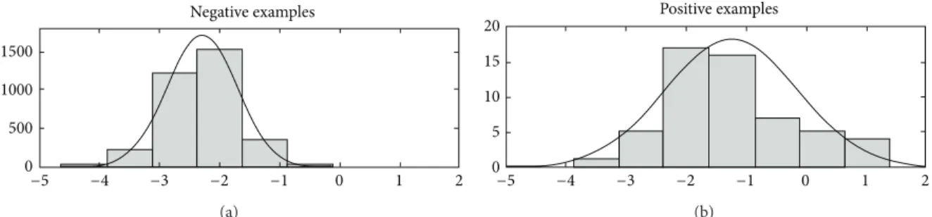
Note that (8) can be inferred from training labels simply

by counting, while (9) can be inferred by validation during

training, by modeling the distribution of ̂𝑦_𝑖 outputs over

positive and negative examples, by assuming a parametric

model (e.g., Gaussian distribution; seeFigure 5).

For the implementation of their method, the authors

adopted bagged ensemble of SVMs [131] to make their

predictions more robust and reliable at each node of the GO hierarchy, and median values of their outputs on out-of-bag examples have been used to estimate means and variances for each class. Finally, means and variances have been used as parameters of the Gaussian models used to estimate the

conditional probabilities of (9).

Results with the 105 terms/nodes of the GO BP (model

organism S. cerevisiae) showed substantial improvements

with respect to nonhierarchical “flat” predictions: the hierar-chical approach improves AUC results on 93 of the 105 GO

terms (Figure 6).

5.2. The Markov Blanket and Approximated Breadth First Solu-tion. In [30], the authors proposed an alternative

approxi-mated solution to the complex equation (7) by introducing

the following two variants of the Bayesian integration: (1) HIER-MB: hierarchical Bayesian combination

involv-ing nodes in the Markov blanket.

(2) HIER-BFS: hierarchical Bayesian combination invo-lving the 30 first nodes visited through a breadth-first-search (BFS) in the GO graph.

1500 1000 500 0 −5 −4 −3 −2 −1 0 1 2 Negative examples (a) −5 −4 −3 −2 −1 0 1 2 Positive examples 20 15 10 5 0 (b)

Figure 5: Distribution of positive and negative validation examples (a Gaussian distribution is assumed). Adapted from [20].

42254 27 7046 6364 6385 30490 16070 16072 164 6396 6397 358 16071 6402 30036 7016 7010 7020 8283 310 282 283 278 82 88 7049 74 87 71 70 7067 67 7059 280 6260 6261 6270 7128 7131 6268 6259 6310 6318 102 6987 7001 6325 6281 6289 7124 1409 6950 6999 6974 6979 6970 6351 45445 16568 6990 6368 6355 6336 6069 6067 6057 6347 6349 122 45944 16579 19538 6461 6464 6457 6736 6412 30163 6513 8468 15885 6447 6414 6413 6508 4511 16182 45545 6897 48193 16081 6887 6893 6889 6891 6088 6906 6605 6806 6911 8623 6108 6809 6610 6607

Figure 6: Improvements induced by the hierarchical prediction of the GO terms. Darker shades of blue indicate largest improvements, and darker shades of red indicate largest deterioration; white means no change (adapted from [20]).

Y1 Y2 Y3 Y4 Y5 Y6 Y7 Y1SVM Y2SVM Y3SVM Y4SVM Y5SVM Y6SVM Y7SVM

Figure 7: Markov blanket surrounding the GO term𝑌₁. Each GO term is represented as a blank node, while the SVM classifier output is represented as a gray node (adapted from [30]).

The method has been applied to the prediction of more than 2000 GO terms for the mouse model organism and

per-formed among the top methods in theMouseFuncchallenge

[2].

The first approach (HIER-MB) modifies the output of the base learners (SVMs in the Guan et al. paper) taking into account the Bayesian network constructed using the Markov

blanket surrounding the GO term of interest (Figure 7).

In a Bayesian network, the Markov blanket of a node 𝑖 is

represented by its parents (par(𝑖)), its children (child(𝑖)), and

its children’s other parents. The Bayesian network involving

the Markov blanket of node𝑖is used to provide the prediction

̂𝑦𝑖 of the ensemble, thus leveraging the local relationships

of node𝑖and the predictions for the nodes included in its

Markov blanket.

To enlarge the size of the Bayesian subnetwork involved in the prediction of the node of interest, a variant based on

Y1 Y2 Y3 Y4 Y5 Y6 Y1SVM Y2SVM Y2SVM Y4SVM Y5SVM Y6SVM

Figure 8: The breadth-first subnetwork stemming from𝑌₁. Each GO term is represented through a blank node and the SVM outputs are represented as gray nodes (adapted from [30]).

the Bayesian networks constructed by applying a classical breadth-first search is the basis of the HIER-BFS algorithm.

To reduce the complexity at most,30terms are included (i.e.,

the first 30 nodes reached by the breadth-first algorithm; see

Figure 8). In the implementation, ensembles of25SVMs have been trained for each node, using vector space integration

techniques [132] to integrate multiple sources of data.

Note that with both HIER-MB and HIER-BFS methods we do not take into account the overall topology of the GO network but only the terms related to the node for which we perform the prediction. Even if this general approach is reasonable and achieves good results, its main drawback is represented by the locality of the hierarchical integration (limited to the Markov blanket and the first 30 BFS nodes). Moreover, in previous works, it has been shown that the adopted integration strategy (vector space integration) is

Data preprocessing

Gene expression microarray Protein sequence and

domain information Protein-protein

interactions Phenotype profiles

Phylogenetic profiles

Disease profiles (using homology) Three classifiers (1) Single SVM for GO termX (2) Hierarchical correction GOX SVMX GOY SVMY (3) Bayesian integration of individual datasets GOX

Data1 Data2 Data3

Ensemble

Held-out set validation to choose the best classifier for each GO

term T rue p o si ti ve ra te

False positive rate

Final ensemble predictions for GO

termX

Figure 9: Integration of diverse methods and diverse sources of data in an ensemble framework for AFP prediction. The best classifier for each GO term is selected through held-out set validation (adapted from [30]).

in most cases worse than kernel fusion [11] and ensemble

methods for data integration [23].

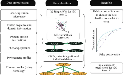
In the same work [30], the authors propose also a sort

of “test and select” method [133], by which three different

classification approaches (a) single flat SVMs, (b) Bayesian hierarchical correction, and (c) Naive Bayes combination are applied, and for each GO term the best one is selected by

internal cross-validation (Figure 9).

It is worth noting that other approaches adopted Bayesian networks to resolve the hierarchical constraints underlying

the GO taxonomy. For instance, in theFALCON algorithm

the GO is modeled as a Bayesian network and for any given input the algorithm returns the most probable GO term assignment in accordance with the GO structure, by using an

evolutionary-based optimization algorithm [134].

5.3. HBAYES: An “Optimal” Hierarchical Bayesian Ensemble Approach. The HBAYES ensemble method [92,135] is a gen-eral technique for solving hierarchical classification problems

on generic taxonomies 𝐺structured according to forest of

trees. The method consists in training a calibrated classifier at each node of the taxonomy. In principle, any algorithm (e.g., support vector machines or artificial neural networks) whose classifications are obtained by thresholding a real prediction

̂𝑝, for example,̂𝑦 =SGN( ̂𝑝), can be used as base learner. The

real-valued outputŝ𝑝_𝑖(𝑔)of the calibrated classifier for node

𝑖on the gene𝑔are viewed as estimates of the probabilities

𝑝_𝑖(𝑔) = P(𝑦_𝑖 = 1 | 𝑦par(𝑖) = 1, 𝑔). The distribution of the

random Boolean vectorY is assumed to be

P(Y=y) =∏𝑚

𝑖=1

P(𝑌_𝑖= 𝑦_𝑖| 𝑌par(𝑖) = 1, 𝑔) ∀y∈ {0, 1}𝑚, (10)

where, in order to enforce that only multilabelsY that respect

the hierarchy have nonzero probability, it is imposed that

P(𝑌_𝑖= 1 | 𝑌par(𝑖) = 0, 𝑔) = 0for all nodes𝑖 = 1, . . . , 𝑚and all

𝑔. This implies that the base learner at node𝑖is only trained

on the subset of the training set including all examples(𝑔,y)

such that𝑦par(𝑖)= 1.

5.3.1. HBAYES Ensembles for Protein Function Prediction. H -loss is a measure of discrepancy between multilabels based on a simple intuition: if a parent class has been predicted wrongly, then errors in its descendants should not be taken

into account. Given fixed cost coefficients𝜃₁, . . . , 𝜃_𝑚> 0, the

H-lossℓ_𝐻(̂y,v)between multilabelŝy and v is computed as

follows: all paths in the taxonomy𝑇from the root down to

each leaf are examined and whenever a node𝑖 ∈ {1, . . . , 𝑚}

is encountered such that̂𝑦_𝑖 ̸=V_𝑖,𝜃_𝑖is added to the loss, while

all the other loss contributions from the subtree rooted at𝑖

are discarded. This method assumes that, given a gene𝑔, the

distribution of the labelsV = (𝑉₁, . . . , 𝑉_𝑚)is P(V = v) =

∏𝑚_𝑖=1𝑝_𝑖(𝑔)for allv ∈ {0, 1}𝑚, where𝑝_𝑖(𝑔) = P(𝑉_𝑖 = V_𝑖 |

𝑉par(𝑖) = 1, 𝑔). According to the true path rule, it is imposed thatP(𝑉_𝑖= 1 | 𝑉par(𝑖) = 0, 𝑔) = 0for all nodes𝑖and all genes 𝑔.

In the evaluation phase, HBAYES predicts the

Bayes-optimal multilabel ̂y ∈ {0, 1}𝑚 for a gene𝑔based on the

estimates ̂𝑝_𝑖(𝑔) for 𝑖 = 1, . . . , 𝑚. By definition of

Bayes-optimality, the optimal multilabel for 𝑔 is the one that

minimizes the loss when the true multilabel V is drawn

from the joint distribution computed from the estimated

conditionalŝ𝑝_𝑖(𝑔). That is,

̂

y=argmin

y∈{0,1}𝑚E[ℓ𝐻(y,V) | 𝑔] . (11)

In other words, the ensemble method HBAYES provides an approximation of the optimal Bayesian classifier with respect

to the H-loss [135]. More precisely, as shown in [27] the

Theorem 1. For any tree𝑇and gene𝑔the multilabel generated according to the HBAYES prediction rule is the Bayes-optimal classification of𝑔for the H-loss.

In the evaluation phase, the uniform cost coefficients

𝜃_𝑖 = 1, for 𝑖 = 1, . . . , 𝑚, are used. However, since with

uniform coefficients the H-loss can be made small simply

by predicting sparse multilabels (i.e., multilabelŝy such that

∑_𝑖̂𝑦𝑖is small), in the training phase the cost coefficients are

set to𝜃_𝑖= 1/|root(𝐺)|, if𝑖 ∈root(𝐺), and to𝜃_𝑖= 𝜃_𝑗/|child(𝑗)|

with𝑗 = par(𝑖), if otherwise. This normalizes theH-loss, in

the sense that the maximalH-loss contribution of all nodes

in a subtree excluding its root equals that of its root.

Let {𝐸} be the indicator function of event 𝐸. Given 𝑔

and the estimates ̂𝑝_𝑖 = ̂𝑝_𝑖(𝑔)for𝑖 = 1, . . . , 𝑚, the HBAYES

prediction rule can be formulated as follows.

HBAYES Prediction Rule.Initially, set the labels of each node

𝑖to ̂𝑦_𝑖=argmin 𝑦∈{0,1} (𝜃𝑖̂𝑝𝑖(1 − 𝑦) + 𝜃𝑖(1 − ̂𝑝𝑖) 𝑦 + ̂𝑝_𝑖{𝑦 = 1} ∑ 𝑗∈child(𝑖) 𝐻_𝑗(̂y)) , (12) where 𝐻_𝑗(̂y) = 𝜃_𝑗̂𝑝𝑗(1 − ̂𝑦𝑗) + 𝜃𝑗(1 − ̂𝑝𝑗) ̂𝑦𝑗 + ̂𝑝_𝑗{ ̂𝑦_𝑗= 1} ∑ 𝑘∈child(𝑗) 𝐻_𝑘(̂y) (13)

is recursively defined over the nodes𝑗in the subtree rooted

at𝑖with eacĥ𝑦_𝑗set according to (12).

Then, if̂𝑦_𝑖is set to zero, set all nodes in the subtree rooted

at𝑖to zero as well.

It is worth noting that̂y can be computed for a given𝑔

via a simple bottom-up message-passing procedure. It can be

shown that if all child nodes𝑘of𝑖havê𝑝_𝑘close to a half, then

the Bayes-optimal label of𝑖tends to be0irrespective of the

value of̂𝑝_𝑖. On the contrary, if𝑖’s children all havê𝑝_𝑘close to

either0or1, then the Bayes-optimal label of𝑖is based on̂𝑝_𝑖

only, ignoring the children. This behaviour can be intuitively

explained in the following way: the estimatê𝑝_𝑘is built based

only on the examples on which the parent𝑖of𝑘is positive;

hence, a “neutral” estimate ̂𝑝_𝑘 = 1/2signals that the current

instance is a negative example for the parent𝑖. Experimental

results show that this approach achieves comparable results

with the TPR method (Section 7), an ensemble approach

based on the “true path rule” [136].

5.3.2. HBAYES-CS: The Cost-Sensitive Version. The HBAYES-CS is the cost-sensitive version of HBAYES proposed in

[27]. By this approach, the misclassification cost coefficient

𝜃𝑖 for node 𝑖 is split into two terms𝜃+𝑖 and 𝜃−𝑖 for taking

into account misclassifications, respectively, for positive and

negative examples. By considering separately these two terms,

(12) can be rewritten as ̂𝑦𝑖=argmin 𝑦∈{0,1} (𝜃 − 𝑖 ̂𝑝𝑖(1 − 𝑦) + 𝜃𝑖+(1 − ̂𝑝𝑖) 𝑦 + ̂𝑝_𝑖{𝑦 = 1} ∑ 𝑗∈child(𝑖) 𝐻_𝑗(̂y)) , (14)

where the expression of𝐻_𝑗( ̂𝑦)gets changed correspondingly.

By introducing a factor𝛼 ≥ 0such that 𝜃−_𝑖 = 𝛼𝜃+_𝑖 while

keeping𝜃+_𝑖 + 𝜃_𝑖− = 2𝜃_𝑖, the relative costs of false positives

and false negatives can be parameterized, thus allowing us to

further rewrite the hierarchical Bayesian rule (Section 5.3.1)

as follows:

̂𝑦𝑖= 1 ⇐⇒ ̂𝑝𝑖(2𝜃𝑖− ∑ 𝑗∈child(𝑖)

𝐻_𝑗) ≥ 2𝜃𝑖

1 + 𝛼. (15)

By setting 𝛼 = 1, we obtain the original version of the

hierarchical Bayesian ensemble and by incrementing 𝛼 we

introduce progressively lower costs for positive predictions. In this way, we can obtain that the recall of the ensemble tends to increase, eventually at the expenses of the precision, and by

tuning the𝛼parameter we can obtain different combinations

of precision/recall values.

In principle, a cost factor 𝛼_𝑖 can be set for each node

𝑖to explicitly take into account the unbalance between the

number of positive𝑛+_𝑖 and negative𝑛_𝑖−examples, estimated

from the training data

𝛼_𝑖= 𝑛_𝑛−𝑖₊ 𝑖 󳨐⇒ 𝜃 + 𝑖 = _𝑛− 2 𝑖/𝑛+𝑖 + 1𝜃𝑖= 2𝑛+_𝑖 𝑛− 𝑖 + 𝑛+𝑖 𝜃𝑖. (16)

The decision rule (15) at each node then becomes

̂𝑦𝑖= 1 ⇐⇒ 𝑝𝑖(2𝜃𝑖− ∑ 𝑗∈child(𝑖) 𝐻𝑗) ≥ _{1 + 𝛼}2𝜃𝑖 𝑖 = 2𝜃𝑖𝑛+𝑖 𝑛− 𝑖 + 𝑛+𝑖 . (17) Results obtained with the yeast model organism showed that HBAYES-CS significantly outperform HTD methods

[27,136].

6. Reconciliation Methods

Hierarchical ensemble methods are basically two-step meth-ods, since at first provide predictions for the single classes and then arrange these predictions to take into account the functional relationships between GO terms. Noble and

colleagues name this general approachreconciliation methods

[24]: they proposed methods for calibrating and combining

independent predictions to obtain a set of probabilistic pre-dictions that are consistent with the topology of the ontology. They applied their ensemble methods to the genome-wide

and ontology-wide function prediction with M. musculus,

( 2 ) SVMs ( 1 ) K er nels

For each term

MGI PPI Pfam

K1 K2 K3 K30 SVM SVM SVM SVM (3) Calibration Probability score,p₂ p1≤ p2; p3≤ p4 p2≤ p5 Y1 Y2 Y3 Y4 Y5 Ontology (4) Reconciliation · · · · · · · · ·

Figure 10: The overall scheme of reconciliation methods (adapted from [24]).

Their goal consists in providing consistent predictions, that is, predictions whose confidence (e.g., posterior prob-ability) increases as we ascend from more specific to more general terms in the GO. Moreover, another important issue of these methods is the availability of confidence values associated with the predictions that can be interpreted as probabilities that a protein has a certain function given the information provided by the data.

The overall reconciliation approach can be summarized

in the following four basic steps (Figure 10):

(1)Kernel computation: at first a set of kernels is com-puted from the available data. We may choose kernel specific for each source of data (e.g., diffusion kernels

for protein-protein interaction data [137], linear or

Gaussian kernel for expression data, and string kernel

for sequence data [138]). Multiple kernels for the same

type of data can also be constructed [24].

(2)SVM learning: SVMs are used as base learners using the kernels selected at the previous step; the training is performed by internal cross-validation to avoid over-fitting, and a local cost-sensitive strategy is applied,

by tuning separately the𝐶 regularization factor for

positive and negative examples. Note that the authors in their experiments used SVMs as base learners but any meaningful classifier could be used at this step.

(3)Calibration: to produce individual probabilistic out-puts from the set of SVM outout-puts corresponding to one GO term, a logistic regression approach is applied. In this way, a calibration of the individual SVM outputs is obtained, resulting in a

probabilis-tic prediction of the random variable 𝑌_𝑖, for each

node/term𝑖of the hierarchy, given the outputs ̂𝑦_𝑖of

the SVM classifiers.

(4)Reconciliation: the first three steps generate unrec-onciled outputs; that is, in practice a “flat” ensemble is applied that may generate inconsistent predictions with respect to the given taxonomy. In this step, the

outputs of step three are processed by a “reconcili-ation method.” The goal of this stage is to combine predictions for each term to produce predictions that are consistent with the ontology, meaning that all the probabilities assigned to the ancestors of a GO term are larger than the probability assigned to that term.

The first three steps are basically the same for (or very similar to) each reconciliation ensemble method. The crucial step is represented by the fourth, that is, the reconciliation step, and different ensemble algorithms can be designed to

implement it. The authors proposed 11 different ensemble

methods for the reconciliation of the base classifier outputs. Schematically, they can be subdivided into the following four main classes of ensembles:

(1) heuristic methods;

(2) Bayesian network-based methods; (3) cascaded logistic regression; (4) projection-based methods.

6.1. Heuristic Methods. These approaches preserve the “rec-onciliation property”

∀𝑖, 𝑗 ∈ 𝐺, (𝑖, 𝑗) ∈ 𝐺 󳨐⇒ ̂𝑝_𝑖≥ ̂𝑝_𝑗 (18)

through simple heuristic modifications of the probabilities computed at step 3 of the overall reconciliation scheme.

(i) The MAX method simply chooses the largest logistic

regression value for the node𝑖and all its descendants

desc

𝑝_𝑖= max

𝑗∈desc(𝑖)̂𝑝𝑗. (19)

(ii) The AND method implements the notion that the

probability of all ancestral GO terms anc(𝑖)of a given

term/node𝑖is large, assuming that, conditional on the

data, all predictions are independent

𝑝_𝑖= ∏

𝑗∈anc(𝑖)

̂𝑝𝑗. ₍₂₀₎

(iii) OR estimates the probability that the node 𝑖 is

annotated at least for one of the descendant GO terms, assuming again that, conditional on the data, all predictions are independent

1 − 𝑝_𝑖= ∏

𝑗∈desc(𝑖)

(1 − ̂𝑝_𝑗) . ₍₂₁₎

6.2. Cascaded Logistic Regression. Instead of modeling class-conditional probabilities, as required by the Bayesian approach, logistic regression can be used instead to directly model posterior probabilities. Considering that modeling conditional densities are in most cases difficult (also using