Maximum Likelihood Estimation of Discrete Log-Concave Distributions with Applications

MAXIMUM LIKELIHOOD ESTIMATION OF DISCRETE

LOG-CONCAVE DISTRIBUTION WITH APPLICATIONS

YAN HUA TIAN

A DISSERTATION SUBMITTED TO THE FACULTY OF GRADUATE STUDIES IN PARTIAL FULFILLMENT OF THE REQUIREMENTS FOR THE

DEGREE OF DOCTOR OF PHILOSOPHY

GRADUATE PROGRAM IN MATHEMATICS AND STATISTICS YORK UNIVERSITY

TORONTO, ONTARIO March 2018

Abstract

Shape-constrained methods specify a class of distributions instead of a single para-metric family. The approach increases the robustness of the estimation without much loss of efficiency. Among these, log-concavity is an appealing shape constraint in dis-tribution modeling, because it falls into the popular unimodal shape-constraint and many parametric models are log-concave. This is therefore the focus of our work.

First, we propose a maximum likelihood estimator of discrete log-concave dis-tributions in higher dimensions. We define a new class of log-concave disdis-tributions on_Zd_{, and study its properties. We show how to compute the maximum likelihood} estimator from an independent and identically distributed sample, and establish con-sistency of the estimator, even if the class has been incorrectly specified. For finite sample sizes, the proposed estimator outperforms a purely nonparametric approach (the empirical distribution), but is able to remain comparable to the correct paramet-ric approach. Furthermore, the new class has a natural relationship with log-concave densities when data has been grouped or discretized. We show how this property can be used in a real data example.

Secondly, we apply the discrete log-concave maximum likelihood estimator in one-dimensional space to a clustering problem. Our work mainly focuses on the categorical nominal data. We develop a log-concave mixture model using the discrete log-concave maximum likelihood estimator. We then apply the log-concave mixture

model to our clustering algorithm. We compare our proposed clustering algorithm with the other two clustering methods. Comparing results show that our proposed algorithm has a good performance.

Contents

Abstract ii

Contents iv

List of Tables vii

List of Figures viii

I

eLC maximum likelihood estimator

1

1 Introduction 2

1.1 Motivation . . . 2

1.2 Overview of maximum likelihood estimation . . . 6

1.3 Background . . . 9

1.3.1 MLE of log-concave density on _Rd _{. . . . 9}

1.3.2 MLE of log-concave mass function on _Z . . . 11

1.3.3 Discrete convex in higher dimensions . . . 15

1.3.4 Generalized log-concave probability mass function . . . 19

2 Introduction of discrete log-concave PMF 23

2.1 Definition of discrete log-concave PMF . . . 24

2.2 Relationship with generalized log-concave PMF . . . 26

2.3 Relationship with continuous log-concave distributions . . . 27

2.4 Properties . . . 29

3 Maximum likelihood estimation of eLC 45 3.1 Computation of the MLE . . . 52

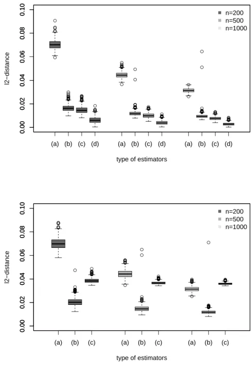
3.2 Finite sample performance . . . 60

3.3 Binned data example . . . 63

3.4 Mixtures and the EM algorithm . . . 64

4 Computing algorithm 65 4.1 Derive the explicit form of σˆy . . . 65

4.2 Derive the explicit form of gradient of σˆy . . . 69

4.3 Subgradient algorithm . . . 74

4.4 Computing algorithm and comparison . . . 75

5 Asymptotic Properties 79

II

Application of discrete log-concave in clustering

90

6.2 Techniques review and background . . . 93

6.2.1 Nominal categorical data set . . . 93

6.2.3 Uniform Hamming distance vector . . . 96

6.2.4 HD vector algorithm . . . 100

6.2.5 K-modes algorithm . . . 106

6.3 Outline . . . 108

7 Log-concave mixture model 110 8 Algorithm 117 8.1 Modified reversed KL divergence . . . 117

8.2 Test cluster pattern using bootstrap . . . 122

8.3 HD-LCD algorithm with the bootstrap . . . 124

8.4 Smoothness and limitations of HD-LCD algorithm . . . 129

9 Clustering result comparison 133 9.1 Algorithm evaluation . . . 133

9.2 Examples for HD-LCD algorithm with the bootstrap . . . 134

9.3 Simulation study . . . 138

9.4 Soybean disease data and zoo data . . . 141

10 Conclusion and future work 145 A Appendix: background material 148 A.1 Important Definitions, Theorems and Lemma . . . 148

A.2 List of important symbols and notations . . . 155

List of Tables

6.1 Example of Hamming distance for zoo data. . . 95

9.1 Examples for HD-LCD algorithm with the bootstrap. . . 137

9.2 Comparison of two simulations . . . 143

9.3 Original simulation study comparison . . . 144

9.4 Modified simulation study comparison . . . 144

9.5 Comparison on soybean disease data . . . 144

List of Figures

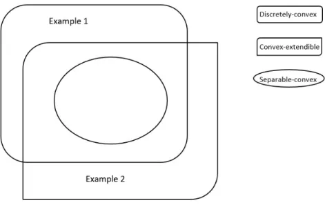
1.1 Relations between three definitions: discrete-convex, convex-extendible, and separable-convex. . . 18 3.1 Grayscale heatmaps of the empirical PMF (left) and its eLC projection

(right). The true distribution is a discrete Gaussian. . . 47 3.2 From the example of Figure 3.1, we compute the marginal

distribu-tions of our eLC MLE, we compare the marginals of elC MLE with empirical marginals and the true marginals in above Figures. . . 48 3.3 Boxplots of l2 distance between estimator and true distribution. . . . 61 3.4 Boston Housing Data: original empirical distribution (left) along with

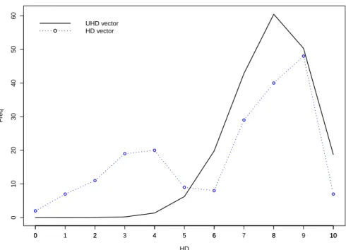
eLC maximum likelihood estimate (right). . . 64 4.1 Subdivisions Sˆy for cases a.(left), b.(centre), and c.(right). . . 67 6.1 UHD with 25 binary attributes . . . 98 6.2 We take one sample (n 200) which is simulated by original simulation

method, we choose one of the simulated center, compare the center’s HD vector against the corresponding UHD vector. . . 99 7.1 Histogram plot against the mixture log-concave projection pÂω.

8.1 Mixture log-concave projection vs empirical distribution of a selected point from Soybean disease data set (1). HD-LCD version cutoffr 7, cluster radius R r2 5. . . 131 8.2 Mixture log-concave projection vs empirical distribution of a selected

point from Soybean disease data set (2). HD-LCD version cutoffr 8, cluster radius R r2 6. . . 132 9.1 (a) is the histogram of modified reversed KL divergence of example

data, computed in the first round, sample size n 60. (b) is the his-togram of largest modified reversed KL divergence of “cluster” samples with sample size of 60. . . 136

Part I

Chapter 1

Introduction

1.1

Motivation

Estimating probability density/mass function is very important in statistics. Para-metric and nonparaPara-metric methods are two popular methodologies in this area. The parametric method is efficient and has good performance, because specific assump-tions are added to the estimation. The disadvantage is that the estimation has large bias when the assumption is wrong. Some example parametric models include: normal distribution, uniform distribution, poisson distributions. The nonparametric method such as the empirical distribution does not need specific parameter assump-tion, is therefore more robust and data-adaptive, but it is not efficient and has larger variance.

Shape-constrained estimation method is one kind of nonparametric method, which means that the probability density/mass function is estimated with some shape-constrained assumptions. The shape constraint includes but is not limited to uni-modality, monotonicity, symmetric, log-concavity. We refer to Wolters and Braun (2017) for the recent works, as well as the advantages and the challenges of shape-constrained estimation models. Grenander (1956) introduced a nonparametric method to estimate the MLE of non-increasing densities, which is known as the Grenander estimator. Other works focused on monotony densities include Groeneboom (1985); Huang and Wellner (1995). Based on the Grenander estimator, later research at-tempted to estimate the unimodal densities. Birg´e (1997) introduced an estimator for estimating non-smooth unimodal densities, when the mode is known. Other works related to unimodal density estimation include Rao (1969); Bickel and Fan (1996).

Note that shape-constrained estimation method stands in the middle of paramet-ric and nonparametparamet-ric methods. Adding shape-constrained assumptions to distri-bution improves the performance and reduces the variance comparing to nonpara-metric method. On the other hand, shape-constrained models specify a larger class than any specific parametric model. Hence comparing to parametric method, it is more robust. For example, Bickel and Fan (1996) introduced density estimation

methods with unimodal shape-constraint and compared their methods with non-parametric kernel estimation. Their methods do a better job for the tail of density and when the distribution is asymmetric. In Section 3.2, we will show that our proposed shape-constrained estimator has an outstanding better performance than the non-parametric estimator, and remains comparable performance comparing to the strong parametric estimator. Of course, there is no guarantee of this in all cir-cumstances. Among those shape constraints, log-concavity is an attractive shape constraint. It includes a wide range of parametric models. For example: normal, uniform, gamma(r, λ) with r C 1, beta(a, b) with a C1, b C 1 in continuous setting, and multinomial, negative multinomial, multivariate hypergeometric in discrete set-ting, they are all log-concave. Furthermore, log-concave densities provide a natural alternative to the class of unimodal densities, while not being too restrictive by spec-ifying a parametric family. Notably, estimating the maximum likelihood estimator of a unimodal density is not an easy problem. Letddenotes the dimension of space, the maximum likelihood estimator does not even exist whend 1, because the like-lihood function can go to infinity (Birg´e, 1997). Log-concave estimation falls in the larger paradigm of shape-constrained estimation, inherits the advantage of striking a balance of efficiency and robustness, also benefits from such properties as (local) adaptivity and not requiring bandwidth.

Walther (2009) introduced the attractive properties of log-concavity and gave a brief review of recent works. For example, Balabdaoui et al. (2009) found the lim-iting distributions of the nonparametric MLE of a log-concave density; Lutz and Kaspar (2011) and D¨umbgen et al. (2007) discussed algorithms and R packages (logcondens) to compute the log-concave MLE in continuous setting; Cule et al. (2010) presented theoretical properties of MLE of log-concave density in multiple dimensional space, developed algorithm to compute the MLE and proved the con-sistency of the MLE; Works of Doss and Wellner (2016) and Kim and Samworth (2016) focused on global convergence rates for the MLE of log-concave densities. For discrete setting, whend 1,Weyermann (2008) showed the existence and uniqueness of the MLE for the log-concave probability mass function (PMF), and provided an active set algorithm to calculate the MLE, which is much in the spirit of D¨umbgen et al. (2007). Balabdaoui et al. (2013) introduced the log-concave MLE of a dis-crete distribution in one dimensional space, and studied consistency and asymptotic properties of the estimator, while Balabdaoui and Jankowski (2016) compared this estimator with the MLE over the class of unimodal probability mass functions on_Z. Among those work, we highlight the works of Cule et al. (2010); Balabdaoui et al. (2013) (will be introduced in the following sections). Our work is much in the spirit of their works. Some of our theoretical results are inspired by the work of Balabdaoui

et al. (2013), for example, the uniqueness, existence and consistency of the MLE. Our algorithm to compute the MLE is much inspired by the work of Cule et al. (2010). We adapt their algorithm and code for discrete setting. In our algorithm, we design and solve the optimization problem following their work. The main difference is that their MLE is in continuous setting, but ours is in discrete setting. More details about the difference will be given in later chapter.

1.2

Overview of maximum likelihood estimation

Maximum likelihood estimation is a well known statistic methodology. With ob-served data, it attempts to estimate distribution and parameters by maximizing the likelihood function. For example, MLE can be used to estimate parameters in a parametric model or the density function with nonparametric shape-constrained methods.

Letx1, ..., xnbenindependent and identically distributed observations from some unknown distribution. We denote the distribution withfˆxSθ, where θ is a param-eter vector. The likelihood function is defined as:

Lˆθ;x1, ..., xn n M i 1

For computation convenience, we apply logarithm to both sides of the function, and obtain the log-likelihood function:

lnLˆθ;x1, ..., xn n Q i 1

lnfˆxiSθ.

The maximum likelihood estimator Âθmle is defined as:

 θmle argmaxθ>Θ n M i 1 fˆxiSθ,

where Θ is the family of parameter θ. Equivalently, maximum likelihood estimator (MLE) can also be expressed by maximizing the average of log-likelihood function:

 θmle argmaxθ>Θ 1 n n Q i 1 lnfˆxiSθ.

The idea behind maximum likelihood estimator is that the most likely parameter maximizes the likelihood function.

MLE is widely used in statistics. Indeed, under certain regulations the MLE has the following properties.

size n large enough. That is,  θmle p Ð θ0, asnÐ ª. ˆ asymptotic normality: º nˆÂθmleθ0 d Ð N ˆ0,Σmle.

ˆ efficiency: MLE is asymptotically efficient since its variance approaches Cramer-Rao lower bound.

Geman and Hwang (1982) mentioned that MLE methodology usually fails when the parameters is in an infinite dimensional space. Hence MLE can not be applied to completely nonparametric statistic models. The MLE of such model does not exist because the likelihood function is unbounded. But situation changes when some constraints are added to the model. MLE works efficiently with shape-constrained nonparametric model. for example Cule et al. (2010) introduced an algorithm to compute the MLE of log-concave densities in multiple dimensional space.

1.3

Background

1.3.1

MLE of log-concave density on

_R

A density function f is said to be log-concave if ˆlogfˆx is a convex function on _Rd_{. A function h is convex if for all x, x}œ >

Rd and for all α > 0,1 it satisfies hˆαx ˆ1αxœ Bαhˆx ˆ1αhˆxœ.LetF denote the set of log-concave density functions on _Rd_{, given x}

1, ..., xn are a random sample drawn from a log-concave density. The log-concave MLE on_Rd _{is defined as:}

 fn argmaxf>F n Q i 1 logfˆxi.

Theorem 1.3.1. (Cule et al., 2010) With probability one, a log-concave maximum likelihood estimatorfn of f0 exists and is unique, where f0 is the true density on Rd.

The above Theorem proved the existence and uniqueness of the log-concave MLE. The algorithm computing the MLE is derived based on the tent functionty. Following Cule (2009), given y>_Rn_{, a tent function can be explicitly defined as}

tyˆx inf˜gˆx RdÐ RS g is concave, and gˆxj Cyj, j 1, ..., n.

is, x1, ..., xn>R2. Hence x1, ..., xn correspond points on a plane. We then put poles with height of y1, ..., yn on those points, respectively. Finally, we stretch a piece of rubber over those poles. The surface of rubber is exactly the tent function for the given y1, ..., yn. The tent function actually reflects concave shape constraint, and it is a piece-wise affine function.

Cule et al. (2010) compute their log-concave MLE by minimizing the objective function over y ˆy1, ..., yn >Rn. The objective function is defined as follows:

σRˆy1, ..., yn 1 n n Q i 1 yi S Cn exp˜tyˆxdx,

where Cn is the convex hull of ˜x1, ..., xn, that is Cn conv˜x1, ..., xn. Note that the objective function is convex (Cule et al., 2010), and it has a unique minimum. Unfortunately, it is proved not to be smooth everywhere, hence many efficient opti-mization techniques can not be applied to this. Subgradient methodology is finally chosen to solve the problem.

The general idea of subgradient algorithms is to proceed iteratively as follows:

Theorem 1.3.2. (Shor, 1985) Let ˆhi be a positive sequence with hi 0 as i ª

formula

yi1 yihi

∂σˆyi Õ∂σˆyi Õ

has the property that either there exists an i0 and y‡ such that yi0 y‡, or yi y‡

and σˆyi σˆy‡ as i ª.

1.3.2

MLE of log-concave mass function on

_Z

In this section we introduce the recent work of log-concave MLE in discrete setting. Whend 1,Weyermann (2008) shows the existence and uniqueness of the maximum likelihood estimator (MLE) for the log-concave probability mass function, and pro-vides an active set algorithm to calculate the MLE, which is much in the spirit of D¨umbgen et al. (2007). Balabdaoui et al. (2013) introduced the log-concave MLE of a discrete distribution in one dimensional space, and studied consistency and asymp-totic properties of the estimator, while Balabdaoui and Jankowski (2016) compare this estimator with the MLE over the class of unimodal probability mass functions on_Z.

To our best knowledge, consideration of log-concave probability mass functions in the multidimensional discrete setting is limited to the work of Bapat (1988), see also Dharmadhikari and Joag-Dev (1988). They defined a class of generalized log-concave distribution. But there is no further study about the property or algorithm

to approximate the distribution. Their definition is a more restrictive class than our proposed definition. More detailed review will be given in later section.

Other than the formal definition of the convex function we mentioned in previous section. Alternatively, if h is twice differentiable, then h is convex if and only if hœœˆx C 0 for all x >_R and if and only if the Hessian matrix of h is positive semi-definite for all x >C, where C is an open convex set on _Rd _{for d} A _{1 (Rockafellar,} 1970, Theorem 4.5, page 27).

Similarly, one can define convex functions in the one-dimensional discrete setting, which naturally leads to a definition of log-concave probability mass functions. That is, letpˆz _Z 0,1denote a probability mass function, where _Zdenotes the inte-gers

˜. . . ,2,1,0,1,2, . . .. The PMFp is said to be log-concave if for any z>_Z

ˆQhˆz hˆz1 2hˆz hˆz1 C 0, (1.1)

where hˆz ˆlogpˆz (Balabdaoui et al., 2013, Proposition 1). In the notation aboveˆQhdenotes the discrete Laplacian operator, which can also be expressed as ˆQhˆz ˜hˆz1 hˆz ˜hˆz hˆz1. This is the second difference of the functionh, and hence this definition matches well that of the continuous setting.

1951) is used to measure the information gain/loss when we use one probability distribution p to approximate another probability distribution p0, which is usually the true distribution. The KL divergence is defined as

ρKLˆpYp0 Q z>Zd p0ˆzlog pˆz p0ˆz .

Although it is not a distance but a divergence, it is the natural notion of “distance” associated with maximum likelihood estimation.

Let P1 denote the class of log-concave PMFs on Z. Balabdaoui et al. (2013) proved the following Theorem.

Theorem 1.3.3. (Balabdaoui et al., 2013) Suppose that p0 is a discrete PMF onZ

with finite mean such that

S Q z>Z

p0ˆzlog˜p0ˆzS @ ª.

Then there is a unique log-concave PMF on _Z, Âp0, such that

Â

p0 argminp>P1ρKLˆpYp0.

divergence and likelihood function, it is not hard to show that the log-concave MLE exists and is unique on_Z. We denote the log-concave MLE (d 1) as pÂn.

Let gˆz denote a finite concave function on _Z. A point K >_Z is a knot of g if gˆK A ª, andg changes slope at K.Further, a knot K is called an internal knot if gˆK 1 A ª and gˆK 1 A ª. Letˆx1, ..., xmbe a random sample from p0,we assume there are m distinct ordered values in the sample: z1 @...@zm.

Discrete concave function gˆz when d 1 can be decomposed to the following form (Balabdaoui et al., 2013):

gˆz abz p Q i 1

ciˆKiz, z>Z9 z1, zm

where a, b > _R and ci @ 0, K1, ...,Kp denote the internal knots of gˆz. Here they used the standard notation z zI_˜zC0. This decomposition is the key to active set algorithm (Weyermann, 2008; D¨umbgen et al., 2007). When d A1 the discrete concavity is defined in a totally different way. The definition of discrete concavity is even not unique. There are no decomposition methods for higher dimensional discrete concave function, hence active set algorithm can not be applied to higher dimensions.

For two PMFs p and p0, we define thelk and Hellinger distances as lkˆp, p0 ¢¨¨¨ ¨¨¨¨ ¦¨¨ ¨¨¨¨¨ ¤ Š Pz>ZdSpˆz p0ˆzS k1~k _{if 1}B_kB ª_, sup_z>ZdSpˆz p₀ˆzS if k ª, h2ˆp, p0 1 2Q_z> Z Š»pˆz »p0ˆz 2 .

Balabdaoui et al. (2013) proved that the log-concave MLE on_Zis consistent in term of the distancelk,0@kB ª or the Hellinger distance.

Theorem 1.3.4. (Balabdaoui et al., 2013) Suppose that p0 is a discrete distribution

on _Z with finite mean such that

S Q z>Z

p0ˆzlog˜p0ˆzS @ ª.

ThendˆÂpn,pÂ0 0almost surely, wheredis the distancelk,0@kB ªor the Hellinger

distance.

1.3.3

Discrete convex in higher dimensions

In higher dimensions, the definition of a discrete convex (equivalently, concave) func-tion is not straightforward. For a discrete funcfunc-tion defined on _Zd _{for d}A_{1 there are} multiple definitions of convexity. Murota and Shioura (2001) provide a detailed

sur-vey of convex functions and sets in the higher-dimensional discrete setting, including a summary of the relationships between the various definitions. Among these def-initions there are three which are relevant to our initial considerations: discretely-convex, separable-discretely-convex, and convex-extendible. To this end, consider a function h_Zd

R8 ˜ª and define the domain domˆh ˜z >ZdShˆz @ ª.

– The function h is said to beseparable-convexif hˆz Pd_{i 1}hiˆzi ˆz >Zdfor a finite family of discrete convex functions hiZ R8 ˜ª,i> ˜1, ..., d. That is,ˆQhiˆz C0 for all z>Z and all i> ˜1, . . . , d.

– For x>_Rd_{, let x (respectively, x) denote the floor (respectively, the ceiling)} of the vector x, obtained by rounding down (respectively, up) each component of x to its nearest integer. Next, define the set N0ˆx ˜z >ZdS x Bz B x. The function h is said to be discretely-convex if, for any zœ, zœœ>domˆh and any α> 0,1, it holds that

min˜hˆz Sz>N0ˆαzœ ˆ1αzœœ B αhˆzœ ˆ1αhˆzœœ.

Similarly, a set S b_Zd _{is said to be discretely-convex if, for any z}œ_{, z}œœ >_{S and} any α> 0,1, it holds thatN0ˆαzœ ˆ1αzœœ 9S is non-empty.

– Define the convex closure ofhˆz

¯

hˆx sup α>R,β>Rd

˜αβTxαβTz Bhˆz for all z >_Zd, x>_Rd.

The function h is convex-extendible if ¯hˆz hˆz for all z > _Zd_{. Similarly,} a set S b _Zd _{is said to be convex-extendible if ¯S}9

Zd S, where ¯S b Rd is the convex closure of S, that is, it is the smallest closed convex set (in _Rd₎ containing S. Another useful definition is convex extension: a closed convex function hR

Rd R8 ˜ª is called a convex extension of h if hRˆz hˆz for all z >_Zd_{. For a discrete convex-extendible function, its convex extension is} a closed continuous convex function which goes through all its points. We may also take a discrete convex-extendible function as a “sub” function of a closed convex function in continuous setting. Note that affine functions are convex. By (Rockafellar, 1970, Theorem 5.5, page 35), the pointwise supremum of an arbitrary collection of convex functions is convex. Hence we conclude that the convex closure ¯his convex. It is also a convex extension ofh.Any convex function is a composition of collections of pointwise affine functions, so convex closure is the greatest convex extension ofh.But clearly not all convex extension is convex closure.

Figure 1.1: Relations between three definitions: discrete-convex, convex-extendible, and separable-convex.

Murota and Shioura (2001) summarize the relationships between the various def-initions of convexity. In particular, some but not all discretely-convex functions are convex-extendible functions and vice versa, while separable-convex functions are both discrete-convex and convex-extendible. Figure 1.1 shows the relations between above three discrete convex definitions. We can see that

Example 1: Consider the set

S ˜z>_Z3Sz1z2z3 2, zi C0, i 1,2,3 8 ˜ˆ1,2,0,ˆ0,1,2,ˆ2,0,1

˜ˆ0,1,1,ˆ1,0,1,ˆ1,1,0,ˆ0,0,2,ˆ0,2,0,ˆ2,0,0,ˆ1,2,0,ˆ0,1,2,ˆ2,0,1.

This set, as well as the function hequal to zero on S and ªon_ZS,are discrete-convex. However, 1 3ˆ1,2,0 1 3ˆ0,1,2 1 3ˆ2,0,1 ˆ1,1,1

is an element of ¯S9_Zd_{, but} ˆ_1,1,1 ~>_{S, and hence h is not convex-extendible.} Example 2: Let S ˜ˆ0,0,ˆ2,1and again define the function h equal to zero onS and ª on_ZS.The convex closure ofS is the segment between points (0,0) and (2,1), hence ¯S9_Zd ˜ˆ_0,0_,ˆ_2,1 ˜_z

1, z2 S, we conclude thath is convex-extendible. On the other hand, N0ˆ0.5z1 0.5z2 N0ˆˆ1,0.5 ˜ˆ1,0,ˆ1,1, whence N0ˆαx

œ _ˆ

1αxœœ 9S g and h is not discrete-convex. Both examples appear in Murota and Shioura (2001).

1.3.4

Generalized log-concave probability mass function

of “generalized log-concavity” on _Nd_{, where}

N denotes the natural numbers. A probability mass functionp on _Nd _{with support} S ˜_z>

Ndpˆz A0, is said to be generalized log-concave if pˆz d M i 1 piˆzi, z> S, (1.2)

where eachpi satisfiesˆQlogpiˆzi B0.That is, each pi is a univariate discrete log-concave function (though not necessarily a PMF - therefore, this is a much different definition than separable-log-concavity from Remark 2.1.1). We will compare our new defined PMF class with generalized log-concave PMF in later chapter.

1.4

Outline

Note that this thesis is divided into two parts, in this Part I, we focus on the maximum likelihood estimator of discrete log-concave distribution in higher dimensions.

In Chapter 2, we give a new definition of log-concave probability mass functions defined on Zd (see Definition 2.1.1). We call this class extendible-log-concave, as it is closely related to extendible-convex functions (Murota and Shioura, 2001). We show that the new definition is equivalent to discrete log-concave distribution when d 1. We introduce a Lemma which can be used to check if a function falls into our new defined class. We

Notably, We show that random variables from a continuous log-concave density can be grouped/binned (e.g. rounded to some accuracy level), the resulted discrete mass function will fall into our new defined distribution class under certain conditions (Proposition 2.3.1). We also show that under which condition the class of generalized log-concave is concave (Proposition 2.2.1). Moreover we prove there exist a unique extendible-log-concave PMF which minimize the distance to a given true PMF in term of KL divergence, and this minimizer is the true PMF itself if the true PMF is extendible-log-concave.

In Chapter 3, we show that the maximum likelihood estimator of our new defined class PMF exists and is unique. We show some attactive properties of the MLE of extendible-log-concave PMF. We discuss how to compute the MLE, and how to derive the objective functions. We compare the performance of our MLE with other parametric and nonpara-metric method through simulations. We developed two simulation scenarios with finite sample size. The proposed MLE exhibits considerable improvement in efficiency over the empirical distribution in the examples we consider. Moreover, in one of the examples we compare our nonparametric MLE to the correct parametric MLE, and the proposed method does not show a great loss of efficiency over the parametric method. Similar behavior was observed by Balabdaoui et al. (2013). In our opinion, this is one of the key benefits of the balance that the log-concave class is able to strike between robustness and efficiency. Fur-thermore we give example to show that our estimator can be applied to “binned/grouped” continuous data set.

form of the objective function and its gradient. We proved that the objective function is convex but not differentiable everywhere. Hence Subgradient methodology is applied to compute the MLE. An R package is developed to make methodology widely available.

In Chapter 5, we prove the consistency of the MLE. If the true PMF is extendible-log-concave, then our MLE converges to the true PMF in term of KL divergence; if the true PMF is not extendible-log-concave, but is close to extendible-log-concave, our MLE still reveals desirable behavior.

Chapter 2

Introduction of discrete log-concave PMF

Our goal here is to define and study discrete log-concave distributions in higher dimen-sions, and we therefore need to select a class of discretely convex (equivalently, concave) functions to work with. Among the various discrete convex definitions introduced by pre-vious chapter, we choose to focus on the class of convex-extendible functions. There are two main reasons for this: It was shown in Murota and Shioura (2001, Theorem 4.1) that the class of convex-extendible functions is closed under addition. Furthermore, using this definition, our class of log-concave probability mass functions is closed under limits. We will show this property later in Theorem 2.4.1.

2.1

Definition of discrete log-concave PMF

Following the definition of convex-extendible function, naturally a function h Zd R8

˜ªis concave-extendible ifh is convex-extendible.

Definition 2.1.1. A PMF pˆz Zd 0,1 is e-log-concave (eLC) if logˆpˆz is

concave-extendible.

In what follows, we letP0 denote the class of all eLC probability mass functions onZd.

Remark 2.1.1 (Separable-log-concavity). When d 1,the class P0 agrees with the class

of discrete log-concave distributions defined in Balabdaoui et al. (2013) by Murota (2009,

Theorem 2.1). The maximum likelihood estimation considered here, when d 1, have

al-ready been studied in Balabdaoui et al. (2013). Furthermore, if aZd-valued random variable

X ˜X1, . . . , Xd has a distribution which is e-log-concave and the elements X1, . . . , Xd

are known to be mutually independent, then the PMF can be written as pˆz eϕˆz,where

ϕˆzis separable-convex. In such a situation, the multivariate MLE problem can be solved

using the work of Balabdaoui et al. (2013). Recall that the active set algorithm is for one dimensional discrete log-concave MLE. We apply active set algorithm to compute each marginal distribution, then get the joint distribution by multiplication of marginal distri-butions. Due to the independence,pˆz

d L i 1Â

piˆzi,where z ˜z1, ..., zd >Zd and pÂiˆzi is

one dimensional log-concave MLE imputed by active set algorithm. Note that

 ϕˆz log˜pˆz log d MpÂiˆzi d Qϕˆzi,

where ϕÂi logpÂi is discrete concave (or eLC). HenceÂϕ is separable-convex. We callpÂas

separable log-concave estimation.

Remark 2.1.2 (Checking the class eLC). The following result gives one simple way to verify if a discrete function is convex-extendible.

Lemma 2.1.1. Murota and Shioura (2001, Lemma 2.3) Let hZd R8 ˜ª be some

function. Then, hˆz hˆz for any z > Zd if and only if there exists a closed convex

extension ofh.

For example, considerhˆz zTAz, where z>Zd, andA is a symmetric dd

positive-definite matrix. The “obvious” convex extension ofhˆz is hRˆ_x _xT_{Axfor x>}

Rd.Note

that by Rockafellar (1970, Theorem 4.5, page 27)hRˆ_x _{is convex. The function is closed}

because it is continuous. By Murota and Shioura (2001, Lemma 2.3) hˆz is therefore,

convex-extendible.

Remark 2.1.3 (Alternative lattice structures). In this work we limit ourselves to the grid Zd, although potentially other lattice structures could also be explored. Simple linear

transformations and rotations are naturally covered by our work. We conjecture that the convex extendible approach could also be applied to more irregular structures, although we do not explore it here. This is particularly attractive in light of the relationship that our definition has with log-concave densities, see Proposition 2.3.1.

Remark 2.1.4 (Unimodality). Several notions of unimodality exist for both densities in

allz>Zd,the probability mass function is equal to

pˆz exp˜hˆz exp˜hRˆ

z,

where hR _{is a convex extension of h}ˆ_z _{defined not only on}

Zd but also onRd.

2.2

Relationship with generalized log-concave PMF

Clearly, the definition of generalized log-concave needs not be restricted to Nd and can easily be extended to Zd. Even with this extension, the definition is still more restrictive than our eLC definition for certain supports. In fact, the following relationship holds.

Proposition 2.2.1. Suppose that p is generalized log-concave with support S. If S is convex-extendible, then p> P0.

Proof. By definition, for anyz> S,we have that

hˆz logpˆz

d Q i 1

˜logpiˆzi

d Q i 1

hiˆzi,

where each piˆzi is discrete log-concave onZ, and hence hiˆzi is discrete convex. Note that the definition of generalized log-concavity does not specify the supportS,which means that S can be any form. Hence we make the assumption that S is convex-extendible to make it work for convex-extendible. For each i, let Si ˜k > Z ˆki > S, where ˆki

denotes any point ofZd with its ith element equal to k. Each functionhi is defined onSi. Hencehˆz Pd_{i 1}hiˆzi is separable-convex onS.Thereforehˆzis convex-extendible by Murota and Shioura (2001), which impliesp> P0.

Based on the Proposition 2.2.1 and the work from Bapat (1988); Johnson et al. (1997), we easily find that distributions such as the multinomial, negative multinomial, multivariate hypergeometric, multivariate negative hypergeometric, as well as multi-parameter versions of the multinomial and negative multinomial are also extendible log-concave. We do this by checking that their supports are convex-extendible set. Hence Proposition 2.2.1 provides another approach to checking if a given probability mass function falls in the classP0.

2.3

Relationship with continuous log-concave

dis-tributions

In the following proposition, we show the relation between our discrete log-concave distri-bution and continuous log-concave distridistri-bution.

Proposition 2.3.1.Suppose thatf is a log-concave density onRd,and letA 1~2,1~2d.

Define the probability mass function pˆz Rz_Afˆydy. Suppose that the support of p is convex-extendible. Then p> P0.

Proof of Proposition 2.3.1. Letf denote a log-concave density onRd.ForA 1~2,1~2d, consider the function qˆx _RxAfˆydy PˆY > Ax, letting Y denote the random

variable with densityf. Then, by the property of log-concave distributions (see e.g. Dhar-madhikari and Joag-Dev (1988, (2.6) on page 47)), for anyα> ˆ0,1 and any x, y>Rd we have that

qˆαx ˆ1αy C qˆxαqˆy1α

which implies that the functionhRˆ_x _logqˆ_x_{is convex. The functionq}ˆ_x_is continu-ous by properties of integrals (applying, for example, the dominated convergence theorem and the fact thatf must be bounded). In fact, lettingB denote an upper bound onf, we have that

Sqˆx qˆyS B B똈Ax∆ˆAy B 4Bdλ˜ASSxySS_ª,

whereλ˜A denotes the Lebesgue measure of the setA, and ∆ denotes set difference sym-bol. It follows that hRˆ_x _logqˆ_x _{is continuous on its effective domain, and therefore} it is lower semi-continuous. Therefore, it is closed (Rockafellar, 1970, Theorem 7.1, page 51) on its effective domain. Lastly, hRˆ_z _logqˆ_x _logpˆ_z _{by definition on}

Zd. It

follows that the restriction ofhR _{to ¯S is a closed convex extension oflogp}ˆ_z_{,and hence}

p> P0 by Murota and Shioura (2001, Lemma 2.3) (Lemma 2.1.1).

A quick look at the proof reveals that our result is not tied to the lattice Zd nor our particular choice of A. Letting Y denote a random variable with density f as above.

Then the PMFpwithA 1~2,1~2dcorresponds to the probability mass function of the random variableX Y0.5(componentwise). Other choices of lattice andAlead to other discretizations ofY,such asδY~δfor someδA0 (this random variable lives on the lattice

δZd. This means that the class P0 can be used to analyze log-concave random variables which have been discretized or “grouped/binned”. An example is given in Section 3.3.

2.4

Properties

The classP0 has several attractive properties.

Proposition 2.4.1. Suppose that p> P0.

1. The support of p, S ˜zSpˆz A0,is a convex-extendible set.

Proof. Let hˆz logpˆz, then hˆz is convex-extendible by assumption, and

S ˜zShˆz @ ª. Hence, by Lemma 2.1.1 (Murota and Shioura, 2001), there exists a convex extensionhRˆxofhˆz,which is a closed convex function onRd.Therefore, the effective domain ofhR,˜xShRˆx @ ª,is a closed convex set inRd(Rockafellar, 1970, page 23 and Theorem 7.1 on page 51). The latter follows since for a closed function, its epigraph must be closed (Rockafellar, 1970, Theorem 7.1 on page 51) and the effective domain is the projection of the epigraph onto Rd, (Rockafellar, 1970, page 23). Since such a projection of a closed set must be closed (appealing to the characterization of closed sets via Cauchy sequences), it follows that the effective

domain is closed. Therefore, S `S b ˜¯ xShRˆx @ ª. Furthermore, we have that S Zd9 ˜xShRˆx @ ª. Therefore, it follows that ¯S 9Zd S, and hence S is convex extendible. 2. For A ` S, let Ç pˆz Œ ¢¨¨¨ ¨¨ ¦¨¨ ¨¨¨¤ pˆz z> A, 0 otherwise. If A is a convex-extendible set, Çp> P0.

Proof. Let hˆz logpˆz, then hˆz is convex-extendible by assumption. By

Lemma 2.1.1 (Murota and Shioura, 2001), there exist a convex extension hRˆ_x _of

hˆz,which is a closed convex function on Rd.We define a function

Ç_hR_ˆ x ¢¨¨¨ ¨¨¨¨ ¦¨¨ ¨¨¨¨¨ ¤ hRˆx logc, x>A¯ ª, x~>A¯, forc _P 1

z>Apˆz,and where ¯A denotes the convex closure ofA.It is obvious thatÇh

R

is also a closed convex function. Also,

logpLjz logˆcpˆz hˆz logc hR_ˆ

z logc ÇhR_ˆ

z,

Ç

p> P0.

3. Let p1 > P0 and p2 > P0 with supports S1 ˜z1 > Zd1Sp1ˆz1 A 0 and S2 ˜z2 > Zd2Sp2ˆz2 A 0. Then pˆz p1ˆz1p2ˆz2 with support S S1 S2 ` Zd1d2 also

satisfiesp> P0.

Proof. Letting h1ˆz1 logp1ˆz1, h2ˆz2 logp2ˆz2 thenh1ˆz, h2ˆz are both convex-extendible by assumption. Let x1 >Rd1, x2>Rd2.By Lemma 2.1.1 (Murota and Shioura, 2001), there exist convex extensions hR

1ˆx1, hR2ˆx2 respectively, of

h1ˆz1, h2ˆz2. These are closed convex functions on Rd1,Rd2. Next, hRˆx1, x2

hR₁ˆx1 hR2ˆx2 is also a convex function on Rd1d2 (see below proof *). Further-more, it is closed, since it is the sum of lower semi-continuous functions, and hence lower semi-continuous (Rockafellar, 1970, Theorem 7.1, page 51). Finally,

hRˆ_z _hR 1ˆz h

R

2ˆz h1ˆz h2ˆz logˆp1ˆz1p2ˆz2 logpˆz,

wherez ˆz1, z2.Thereforep> P0.

Letxœ, xœœ >Rd1d2, xœ1, x œœ 1 >Rd1, x œ 2, x œœ 2 >Rd2 andx œ ˆxœ₁, xœ₂, xœœ ˆxœœ₁, xœœ₂. hRˆαxœ ˆ1αxœœ hRˆαxœ₁ ˆ1αxœœ₁, αx₂œ ˆ1αxœœ₂ hR₁ˆαxœ₁ ˆ1αxœœ₁ hR₂ˆαxœ₂ ˆ1αxœœ₂ @αhR₁ˆxœ₁ ˆ1αhR₁ˆxœœ₁ αhR₂ˆxœ₂ ˆ1αhR₂ˆxœœ₂ αˆhR₁ˆxœ₁ hR₂ˆxœ₂ ˆ1ፈhR₁ˆxœœ₁ hR₂ˆxœœ₂ αhRˆxœ₁, xœ₂ ˆ1ፈhRˆxœœ₁, xœœ₂ αhRˆxœ ˆ1αhRˆxœœ

4. Suppose that p> P0 with support inZdand letz ˆz1, z2 wherez1>Zd1 andz2>Zd2

withd1d2 d. Then the conditional distributionpˆz1Sz2 pˆˆz1, z2~pˆz2 > P0.

Proof. Let hˆz logpˆz, then hˆz is convex-extendible by assumption and fix

z2 > Zd2. By Lemma 2.1.1, there exists a convex extension hRˆx of hˆz, which is a closed convex function on Rd. Let p2 denote the marginal of p p2ˆz2 Pz1>Zd1pˆz1, z2.We then defineÇh

Rˆ_x

1 hRˆx1, x2 z2logp2ˆz2,wherex1>Rd1, and z2 > Zd2 ` Rd2 is fixed. We will show that ÇhR is the convex extension of

Firstly, we have that for anyz1>Zd1

Ç_hRˆ

z1 hRˆz1, z2 logp2ˆz2 logpˆz1, z2 logp2ˆz2 logpˆz1Sz2.

Secondly,ÇhRˆ_x

1 is convex since hRˆx is convex in x1 and logp2ˆz2 is a constant. Finally, we need thatÇhR_{is closed. This follows from Rockafellar (1970, Theorem 7.1,} page 51) by appealing to the definition of closed sets via Cauchy sequences.

Note that hRˆx hRˆx1, x2 is closed implies the level set of hRˆx1, x2 is closed, let denote the level set as C ˜ˆx > RdShRˆx B α, α @ ª. By Krantz (1991, Proposition 5.5), for any Cauchy sequence˜xninsideC,wherexi ˜xi1, xi2, ..., xid, fori 1,2, ..., n, ...,it’s limitx0 ˜x01, x02, ..., x0dis also an element ofC.

For a fixz2 ˜z21, ..., z2d₂ >Z

d2_{, we firstly show that h}R_ˆx

1, z2 is closed. For the sameα,the level set ofhRˆx1, z2can be expressed by ˜C ˜x1>Rd1ShRˆx1, z2 Bα. Note that chosen ofz2 may lead to a empty level set ofhRˆx1, z2,we then consider two cases:

(a) ifˆx1, z2 ~>C,then ˜C g,which is closed.

(b) ifˆx1, z2 >C,then for each Cauchy sequence ˜x˜n inside ˜C, where ˜

xi ˜x˜i1, ...,x˜id₁, we can extend it to a d dimensional Cauchy sequence˜xn withxi ˜x˜i1, ...,x˜id1, z21, ..., z2d2, i 1,2, ..., n, ...Note that˜xn>C,hence its

limit, denoted by x0 ˜x01, ..., x0a, z21..., z2d₂ ˆx˜0, z2,is inside C. We then have hRˆx˜0, z2 B α. We conclude that ˜x0 > C.˜ By the process we construct ˜

x0,it is obviously the limit of Cauchy sequence ˜x˜n.Hence by Krantz (1991, Proposition 5.5), ˜C is closed.

Therefore hRˆx1, z2 is closed. It is obvious that ÇhRˆx1 hRˆx1, z2 logp2ˆz2 is also closed since logp2ˆz2is a constant.

Hence our constructed functionÇhR is a closed convex function, and is the convex extension oflogpˆz1Sz2.Hence pˆz1Sz2 is also eLC.

5. Let Z be a discrete random variable, with probability mass function p > P0 with

supportS. Consider the linear transformationZÇ AZb, where Ais a dd matrix

andb is a vector of length d. Let Çp denote the PMF of ZÇ with support SÇ.If

(a) SÇis a subset of Zd,

(b) the matrixA is invertible,

thenÇp> P0.

Proof. Firstly, we add the first condition because our work focus on Zd. We need

work to other the lattice structure (which is possible), this condition can be removed easily.

Let hˆz logpˆz, then hˆz is convex-extendible by assumption. Hence, by Lemma 2.1.1 (Murota and Shioura, 2001), there exists a convex extension hRˆ_x _of

hˆz,which is a closed convex function. Note thatpLjz pˆA1ˆzbfor anyz> ÇS.

We then constructÇhRˆ_x _hRˆ_A1_{ˆxb, for anyx>convˆ ÇS,whereS}Ç_{denote the} convex hull ofS Clearly,ÇhR _{is also convex and closed. Moreover,}

ÇhR_ˆ

z hR_ˆ

A1ˆzb hˆA1ˆzb logpˆA1ˆzb logpLjz,

for any z>Z.Hence ˜hR is the convex extension ofp,Ç and therefore Çp> P0.

The following Theorem shows that the class P0 is closed under limits under some assumptions.

Theorem 2.4.1. Let pnˆn 1,2, ..., p be discrete PMFs on Zd,and suppose that for each nC1, pn> P0. If pn p pointwise and the support of p is convex-extendible, then p> P0.

Proof. Define S0 ˜z>ZdSpˆz A0 and assume (for the moment) that S0 Zd. Define alsohnˆz logpnˆz,for eachnC1 andhˆz logpˆz.By assumption, hn is convex-extendible, and converges to h pointwise on S0.To prove that p is eLC, we need to show

that h is convex-extendible. To do this, we will use Lemma 2.1.1 (Murota and Shioura, 2001), and find a closed convex extension ofh.

By Lemma 2.1.1 (Murota and Shioura, 2001), there exists a closed convex extension of

hn,for eachn. We denote this byhRnRd R8 ˜ª.By definition,hRn is a closed convex function, andhRnˆ_z _hnˆ_z _{for any z}>

Zd.

Fix K>Z to be a large, positive integer, and let BK ˜x>Rd YxYªBK,a closed

(in Rd) and bounded set. Since pn p for all z >Zd,there exists an n0 such that for all

nCn0, pnˆz A0, and hencehnˆz @ ªfor all z> BK.

Note thatBK is a subset ofRd,and also the convex hull ofBK9Zd(inRd). Since each hR

nis closed and convex, we can apply Theorem A.1.8 (Rockafellar, 1970) in the Appendix, and conclude that for eachn,

sup x>BK hR_nˆ x B sup z>BK9Zd hR_nˆ z sup z>BK9Zd hnˆz. Therefore, sup nCn0 sup x>BK hR_nˆ x B sup nCn0 sup z>BK9Zd hnˆz MK,n0, (2.1)

where MK,n0 is finite because S0 Zd. Therefore the sequence ˜hRnˆxnCn0 is finite and pointwise bounded (uniformly) for all x > BK. The statement continues to hold on the relative interior ofBK (again, inRd), which we denote rlBK.By Rockafellar (1970,

Theo-rem 10.6, page 88), TheoTheo-rem A.1.4 in the Appendix, we conclude thathRnˆ_x _{is uniformly} bounded and equi-Lipschitzian relative to, say, BK1. By the Arzel`a-Ascoli theorem, we conclude that hR

n is compact and hence there is a subsequence of h R

n that converges uni-formly onB_ˆK1.We denote this subsequence ashR

nK,and its limit as h R_.

We now argue thathRˆ_x_{is a convex extension of h}ˆ_z _on B

ˆK1 : — SincehR _{is the limit of a sequence of convex functions defined on}B

ˆK1, it follows that hR _{is convex on} B ˆK1. — By definition,hRˆ_z _lim nK ªh R

nKˆz limnK ªhnKˆz hˆz, for any z> BˆK1. — For anyK, hR

nKˆxis finite by inequality (2.1). We also know that it is continuous and uniformly converges to hRˆ_x _on B

ˆK1. Hence hRˆx is also finite, and continuous on B_ˆK1by Krantz (1991, Theorem 9.1, page 201), and thereforehRˆxis closed onBˆK1 by the definition of continuous functions (Krantz, 1991, Theorem 6.9, page 142). Hence we can conclude thathRˆ_x_{is a closed convex extension ofh}ˆ_z_onB

ˆK1.Therefore

hˆz is convex-extendible by Murota and Shioura (2001, Lemma 2.3). Recall thathˆz

logpˆz,we conclude thatpˆz is also eLC forz> B_ˆK1. Since the above conclusion is true for anyK>Z, thereforepˆz is eLC forz>Zd.

Now we consider the situation thatS0`Zd.Note thatpn is eLC, hence the supportSn is convex-extendible set by Proposition 2.4.1 1. Therefore, there exists a convex closure ¯Sn of Sn, which is closed and convex on Rd.For large enough n0, We may repeat the above proof, but considering BK 9Sn0¯ instead of BK throughout. Note that BK is closed and

convex by definition, and intersection of two closed convex sets is also closed and convex. The proof may now be repeated as above, andh will be convex-extendible on Sn0,which equals toS0 eventually.

LetYzY_ª denote maximum norm, YzY_ª max˜Sz1S, ...,SzdS.

Theorem 2.4.2. Let p0 be a probability mass function on Zd such that Pz_>ZdYzYªp0ˆz @ ª andS Pz_>Zdp₀ˆzlogp₀ˆzS @ ª.Suppose also that the convex hull of the support of p₀ is

closed. Then, there exists a uniquepÂ0,such that

Â

p0 argmin p>P0

ρKLˆpÕp0. (2.2)

Furthermore, ifp0 > P0, then pÂ0 p0.

We will refer to pÂ0 as the KL projection of p0 in what follows. Heuristically, the KL projection is the closest element of the classP0 to the fixed PMFp0.

Before we proof this Theorem, we will give the proof of a Lemma.

Lemma 2.4.1. Suppose p1, p2 > P0. Then a PMF p Œ ˆp1p2α for any α > ˆ0,1 also

satisfiesp> P0.

Proof. Let h1 logp1, h2 logp2 and h αˆh1 h2 c (defined on Zd) for some

(respectively), which exist by assumption. ThenhR _αˆ_h

1Rh2R cis closed, convex (see previous proof of *), and by definition satisfies

hR_ˆ

z αˆh1Rˆz h2Rˆz c αˆh1ˆz h2ˆz c hˆz logpˆz

onZd.Therefore,p> P0.

We now proof the Theorem 2.4.2.

Proof of Theorem 2.4.2. We firstly prove the existence part of the theorem. LetS0 ˜z>

ZdSp0ˆz A0denote the support of p0.Without loss of generality, we assumeS0 Zd.Let

Ç

q ŒeYzYª_{, where z> Z}d_{,such that Çq x Âp}

0 (if pÂ0 ŒeYzYª,then we can put qnje0.5YzYª instead, say). Note that logÇqˆz YzY_ª, and since all norms on Rd are closed convex functions, YxY_ª, x > Rd is a convex extension of YzYª. Hence Çq is eLC by Murota and Shioura (2001, Lemma 2.3).

We can also show thatρKLˆÇqÕp0 @ ªunder our assumption.

ρKLˆÇqÕp0 Q z>Zd p0logp0ˆz Q z>Zd p0logÇqˆz Q z>Zd p0logp0ˆz Q z>Zd YzY_ªp0ˆz @ ª. Hence, infq>P0ρKLˆqÕp0 @ ª.

Therefore, there exists a sequence of eLC PMFs˜qn, such that

ρKLˆqnÕp0 inf q>P0

ρKLˆqÕp0.

Because infq>P0ρKLˆq Õp0 @ρKLˆÇq Õp0, there exists an N A0, such that for all nAN, we have

ρKLˆqnÕp0 B ρKLˆÇqÕp0.

Because bothlogqnˆz,logÇqˆzare positive, hence,

sup nAN_zQ_>Zd S logqnˆzSp0ˆz B Q z>Zd S logqLjzSp0ˆz Q z>Zd YzY_ªp0ˆz @ ª.

Let M A0 and consider SM ˜z YzY_ªBM.Let αM minz>SMp0ˆz, and note that asM ª,we have thatαM 0,since p0 is summable. It follows that

sup nAN_z>SQ_MS logqnˆzS B œmax z>SM 1 p0ˆz¡ ¢¨¨ ¦¨¨ ¤ sup nAN_zQ_>SMS logqnˆzSp0ˆz£¨¨§¨¨ ¥ B œmax z>SM 1 p0ˆz¡ ¢¨¨ ¦¨¨ ¤ sup nAN_zQ_> Zd S logqnˆzSp0ˆz£¨¨§¨¨ ¥ B œmax z>SM 1 p0ˆz¡ ¢¨¨ ¦¨¨ ¤zQ>Zd YzY_ªp0ˆz£¨¨§¨¨ ¥ B αM ,

whereB Ep0 YZYª @ ª.Hence, sup nAN sup z>SM S logqnˆzS BB~αM, expœsup nAN sup z>SM S logqnˆzS¡ Cexp˜B~αM. Hence inf nANxmin>SM qnˆz CeB~αM _δ M.

Furthermore, we can find an integerM1AM large enough so that

sup nAN sup z>Sc M₁ qnˆz @δM~2.

Therefore, we can find an envelope functionelˆz,wherelˆz αYzY_ªβ withα, β>R, such that sup_nANqnˆz Belˆz.

Let Xn be a sequence of random vectors with PMF qn. Since elˆz is summable it follows that Xn is tight. Hence, there exists a convergent subsequence qnl, and a limit pointq0 (Rosenthal, 2006). As qn is eLC, by Theorem 2.4.1q0 is also eLC.

By Fatou’s lemma, we have

ρKLˆq0Õp0 Q z>Zd p0log p0 q0 B lim inf nl _zQ_> Zd p0log p0 qnl lim inf nl ρKLˆqnlÕp0.

is, a minimizerÂp0 exists, and the proof of existence is done.

We now prove uniqueness. Let’s assume thatÂp1,pÂ2 are both eLC and minimize ρKLˆ Õ

p0.Let ÇpŒ ˆÂp1pÂ21~2 is a proper PMF. Note that by Lemma 2.4.1,Çp is also eLC. Now,

ρKLˆÇpÕp0 Qp0log p0 Ç p ˆ1~2 Qp0log p0  p1 ˆ 1~2 Qp0log p0  p2 logQˆÂp1Âp21~2 ρKLˆÂp1Õp0 logQˆÂp1Âp21~2 B ρKLˆÂp1 Õp0.

The last inequality follows that PˆÂp1Âp21~2 B P Âp1P Âp2 1 by Cauchy-Schwarz. However, sinceρKLˆÇpÕp0 CρKLˆÂp1Õp0,we find thatPˆÂp1Âp21~2 P Âp1P Âp2 1.ThereforepÂ1 pÂ2, again by Cauchy-Schwarz. This completes the proof.

The following lemma characterizes the support of Âp0.

Lemma 2.4.2. The support of the KL projection Âp0 is the intersection of Zd with the

(closed) convex hull of S0,which is the support of p0.

Proof of Lemma 2.4.2. LetSÂ0 denote the support ofÂp0.LetSÇ0 convˆS0 9Zd. Our goal is to show thatSÂ0 SÇ0.Here, we denote the convex hull ofS0 as convˆS0,and note that by assumption, this is closed.

Firstly, note that if p0ˆz0 A0, then Âp0ˆz0 A0 (we call this fact one). This follows directly from the form of the KL divergence, as PMFs with support strictly smaller than that of p have an infinite KL divergence, and can therefore not act as minimizers. We

thus have thatS0b ÂS0.

Next, consider there exists z0 > ÇS0 convˆS0 9Zd, but z0 ~> ÂS0, that is pÂ0ˆz0 0. Then by Carath´eodory’s Theorem (Rockafellar, 1970, Theorem 17.1 page 155) we can write z0 Pdi11λizi,where λi A0,Pid11λi 1 and zi > S0 for each i 1, . . . , d1.Since Âp0 is eLC and therefore logpÂ0 has a concave extension equal to logpÂ0 on Zd. By the concave property of the concave extension, we find that

logpÂ0ˆz0 logÂp0ˆ d1 Q i 1 λizi C d1 Q i 1 λilogpÂ0ˆzi.

But then Âp0ˆz0 0 implies that logÂp0ˆz0 ª and hence pÂ0ˆzi 0 for at least one 1BiBd1. But p0ˆzi A0 because zi > S0. This is a direct contradiction with fact one. It follows that SÇ0 S0b ÂS0.Together withfact one (S0b ÂS0), this yieldsSÇ0b ÂS0.

Finally, consider a z0>Zd such that z0> ÂS0,that ispÂ0ˆz0 A0.But z0 ~> ÇS0.Construct a PMF Ç pˆz ¢¨¨¨ ¨¨¨¨ ¦¨¨ ¨¨¨¨¨ ¤ cpÂ0ˆz z> ÇS0 0 z~> ÇS0

Also, note thatcA1 by assumption, hence Çpˆz A Âp0ˆz.Then, ρKLˆÂp0Õp0 Q z>Zd p0ˆzlogp0ˆz Q z>Zd p0ˆzlogÂp0ˆz ρKLˆÇpÕp0 Q z>Zd p0ˆzlogpLjz Q z>Zd p0ˆzlogpÂ0ˆz ρKLˆÇpÕp0 Q z>Zd p0ˆzšlogÇpˆz logÂp0ˆzŸ ρKLˆÇpÕp0 Q z>S0 p0ˆz ˜logÇpˆz logÂp0ˆz A ρKLˆÇpÕp0.

Therefore,pÂ0 cannot minimize the KL divergence. Therefore, SÂ0 b ÇS0. Together with the previous conclusionSÇ0 b ÂS0,we have SÇ0 SÂ0.

Chapter 3

Maximum likelihood estimation of eLC

Note that the convex hull of a finite number of points is a closed polygon, from which it follows that the support of the empirical distribution is convex-extendible. The following result is thus a simple consequence of Theorem 2.4.2.

Proposition 3.0.1. Suppose that X1, . . . , Xn are independent and identically distributed

random variables onZd with true PMFp0.Then, with probability one, there exists a unique

eLC maximum likelihood estimator. That is, there exists a unique Âpn which maximizes the

likelihood Ln

i 1

pˆXi over the class of probability mass functions p> P0. In what follows, we will use the notation Âpn to denote the MLE

 pn argmaxp>P0 n Q i 1 logpˆXi.

can show that minimizing KL divergence between eLC PMF and the empirical distribution is equivalent to maximizing the likelihood function.

 pn argminp>P0ρKLˆpÕp¯n argminp>P0ˆ Q z>Zd ¯ pnlogp Q z>Zd ¯ pnlog ¯pn, is equivalent to  pn argminp>P0ˆ Q z>Zd ¯ pnlogp, which is equivalent to  pn argmaxp>P0 1 n_zQ_> Zd logp.

Therefore the existence and uniqueness of eLC MLE is a quick consequence of Theorem 2.4.2.

Computation of this estimator is, unfortunately, not an easy problem. We again refer to Walther (2009) for a review. In d 1, for example the active set algorithm tends to rely on a special structure of convex functions which holds only for d 1. For dA1, this computational problem was first solved in Cule et al. (2010), and it is their approach which we adapt to the discrete setting in this work. This is described in more detail in the next chapter.

The following is another useful property of the eLC MLE, also known to hold in the continuous and discrete d 1 cases.

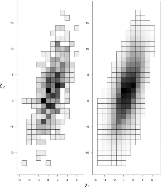
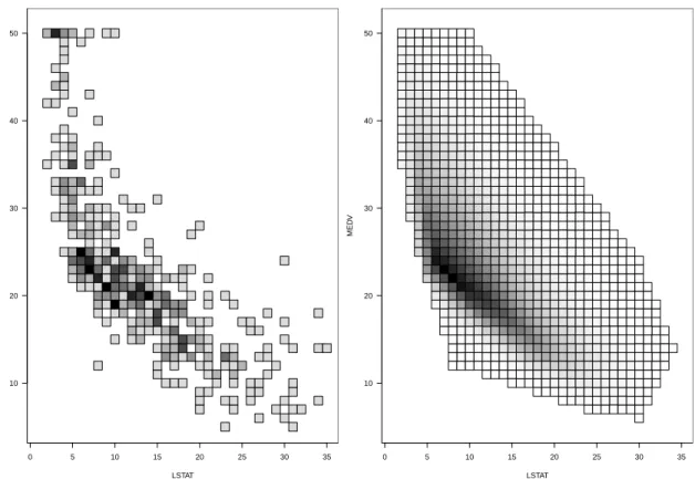
Figure 3.1: Grayscale heatmaps of the empirical PMF (left) and its eLC projection (right). The true distribution is a discrete Gaussian.

0.00 0.05 0.10 0.15 0.20 z1 Prob −6 −5 −4 −3 −2 −1 0 1 2 3 4 5 6 7 empirical eLC MLE truth 0.00 0.05 0.10 0.15 0.20 Z2 Prob −14 −11 −9 −7 −5 −3 −1 1 3 5 7 9 11 13 15 17 19 empirical eLC MLE truth

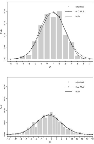
Figure 3.2: From the example of Figure 3.1, we compute the marginal distributions of our eLC MLE, we compare the marginals of elC MLE with empirical marginals and the true marginals in above Figures.

random variablesX1, ..., Xn on Zd, let hZd(R be any convex-extendible function, then Q z>Zd hˆz Âpnˆz B Q z>Zd hˆzp_nˆz.

Proof. First, note thatÂpn is obtained by maximizing the following functional

ֈϕ n Q i 1 ϕˆzip¯n Q z>Zd exp˜ϕˆz

over all concave-extendible functions, where ϕˆz logpˆz ( see Lemma 3.1.1). Letting Â

ϕn argmax ֈϕ,we then haveÂpnˆz exp˜Âϕnˆz.

Letgˆz Zd(Rbe any concave-extendible function, and hence for anyεA0, ϕεg is also concave-extendible (Murota and Shioura, 2001, Theorem 4). Therefore, ֈÂϕnεg B

ֈÂϕn sinceϕÂn maximize Φ. This implies that lim ε 0 ֈÂϕnεg ֈÂϕn ε lim ε 0 n P i 1˜Â ϕnˆzi εgˆzip¯n P z>Zd exp˜Âϕnˆz εgˆz Pn i 1 ϕnˆzip¯n P z>Zd exp˜Âϕnˆz ε n Q i 1 gˆzip¯nlim ε 0 Q z>Zd exp˜Âϕnˆz εgˆz exp˜Âϕnˆz ε n Q i 1 gˆzip¯n Q z>Zd gˆzexp˜Âϕn n Q i 1 gˆzip¯n Q z>Zd gˆzÂpn Q z>Zd gˆzp¯n Q z>Zd gˆzÂpn B 0.

Note that the third last equality comes from:

lim ε 0 exp˜Âϕnˆz εgˆz exp˜Âϕnˆz ε exp˜Âϕnˆzlim ε 0 exp˜εgˆz 1 ε exp˜Âϕnˆzlim ε 0 gˆzexp˜εgˆz 1 gˆzexp˜Âϕnˆz

Similarly, for any convex-extendible functionh,we have

Q z>Zd

hˆzÂpn B Q z>Zd

In particular, this implies that the mean of the MLE is equal to the observed mean of the data, because affine functionshˆz z, z>Zd are both convex-extendible and concave-extendible functions. Hence we have

E_Âpnˆz Q z>Zd zÂpnˆz BEp¯nˆz Q z>Zd zp¯nˆz, E_Âpnˆz Q z>Zd zÂpnˆz CEp¯nˆz Q z>Zd zp¯nˆz. HenceEp_Ânˆz Ep¯nˆz.

Furthermore, the following Lemma shows that the variance matrix under the eLC MLE is smaller than the variance matrix under empirical distribution, in the sense that Σn ÂΣn is positive semi-definite.

Lemma 3.0.2. let ΣÂn denotes the variance matrix of random variable which follows the

distributionpÂn. LetΣn denotes the empirical variance matrix, which is the variance matrix

of random variable following the empirical distributionp_n. Then Σn ÂΣn is positive

semi-definite.

Proof. Let V be any non zero vector on Rd, we define function hˆz VTzzTV, z > Zd. Note thathˆzis convex-extendible, becausehˆz ˆzTVTˆzTV ˆzTV2, it has convex extensionhˆx ˆxTV2, x>Rd,which is closed convex function onRd.

Hence Q z>Zd hˆzÂpnB Q z>Zd hˆzp¯n, Q z>Zd VTzzTVpÂn Q z>Zd VTzzTVp¯nB0, VTˆ Q z>Zd zzTpÂn Q z>Zd zzTp¯nV B0.

Therefore Σn ÂΣn is positive semi-definite.

An example of the MLE is given in Figures 3.1 and 3.2. The data is an IID sample of size n 1000 from the discrete Gaussian distribution given on later Section. Figure 3.1 shows the empirical distribution (left) and the fitted eLC (right) as a grey-scale heatmap. The marginal distributions are given in Figure 3.2, where the true marginals are also added.

3.1

Computation of the MLE

For shape constraint method, it is a standard trick to add a summation term to the log-likelihood function, such that the optimization problem can be relaxed to general functions set instead of density functions set. That is, maximizing

n P i 1

equiv-alent to minimizing 1 n n Q i 1 ϕˆXi Q z>Zd exp˜ϕˆz, (3.1)

over all concave-extendible functionsϕ. Complete proof please see below Lemma 3.1.1. Note, however, that the valuesX1, . . . , Xnare expected to have duplicates in our setting. Therefore, letz1, . . . , zm denote the unique observed values of X1, . . . , Xn.

Lemma 3.1.1. When the criterion function

ֈϕ m Q j 1 wjϕˆzj Q z>Zd eϕˆz

is minimized over all concave extendible functionsϕ, the minimizer satisfies P

z>Zd

eϕˆz 1.

Proof. Consider any concave extendible ϕ0 minimize ֈϕ, and p0 exp˜ϕ0 such that

P z>Zd

exp˜ϕ0ˆz cx1.LetϕÇ0 ϕ0logc.ThenPz_>Zdexp˜Çϕ₀ˆz 1,because Q

z>Zd

exp˜Çϕ0ˆz Q z>Zd

expšexp˜ϕ0ˆz logcŸ

Q z>Zd exp˜ϕ0ˆz c 1 c_zQ_> Zd exp˜ϕ0ˆz 1

Now, ֈÇϕ0 m Q j 1 wjϕÇ0ˆzj Q z>Zd eϕ0Ljz Qm j 1 wj™ϕ0ˆzj logcž 1 m Q j 1 wjϕ0ˆzj m Q j 1 wjlogc1 m Q j 1 wjϕ0ˆzj logc1 m Q j 1 wjϕ0ˆzj Q z>Zd eϕ0ˆz Q z>Zd eϕ0ˆzlogc1 ֈϕ0 clogc1.

Since logcBc1 for any cA0,we get ֈÇϕ0 Bֈϕ0,which is a contradiction.

Let Sn Sn¯ 9Zd, where Sn ˜z1, . . . , zm. Also recall the empirical PMF pn. Using also the characterization of the MLE, we can further re-write the optimization problem above to be equivalent to minimizing

ֈϕ m Q j 1 pnˆzjϕˆzj Q z> ÂSn exp˜ϕˆz,

again, over all concave-extendible functionsϕ. We denote the minimizer of above function asϕˆz logÂpn.

defined as

tyˆx inf˜gˆx Rd RSg is concave, andgˆzj Cyj forj 1, . . . , m.

It turns out, that in the above we can exchange the function ϕˆz with the tent func-tions tyˆz, and optimize over the vector y > Rm instead. Lemma 3.1.2 shows a further simplification of the optimization problem .

Lemma 3.1.2. Consider the function

τˆy1, . . . , ym m Q i 1 wjtyˆzj Q z>ÂSn exp˜tyˆz. (3.2)

Then τ has a minimum over y > Rm. We denote the minimizer as Ây, and pÂnˆz

exp˜t_Âyˆz. Furthermore, tÂy is a concave extension of logpÂn.

Proof. LetϕÂn logÂpn,which minimizes ֈϕ.LetÂyi ϕÂnˆzi,fori 1, . . . , m,and consider

t_Âyˆx inf˜gˆx Rd(RSg is concave, andgˆzi C Âyi for i 1, . . . , m. LetϕÂR

nRd(Rdenote the concave extension ofϕÂn,and note thatϕÂRnˆzi Âϕnˆzi Âyi, i 1. . . , m. ThereforeϕÂR

n belongs to the set

Ast_Ây is the infimum of the above class of functions, we have tyˆz B ÂϕRnˆz, z>Zd. Assume that for some z0>Zd,ϕÂnˆz0 Atyˆz0.Then P

z>Zd

expϕÂnˆz A P

z>Zd

exp˜t_Âyˆz.

Also note thatty_ˆzi C Âyi, i 1, ..., m. Hence ֈÂϕn m Q i 1 wiϕÂnˆzi Q z>Zd expϕÂnˆz Qm i 1 wiÂyi Q z>Zd expϕÂnˆz A Qm i 1 witÂyˆzi Q z>Zd exp˜t_Âyˆz ֈt_Ây.

However, this creates a contradiction since ϕÂn minimizes Φ. Therefore, ϕÂnˆz tÂyˆz, for any z>Zd.This also implies thattyÂis a concave extension of logpÂn.

While the above τ function has extended our optimization problem over y > Rm. It is still not simple enough for computation purpose. We show the objective function in the following Theorem 3.1.1 is convex. Because of convexity, the objective function has a unique minimizer. This objective function is the one we will work on in the sequel.

Theorem 3.1.1. Consider the function

σˆy1, . . . , ym m Q j 1 pnˆzjyj Q z>ÂSn exp˜tyˆz. (3.3)

Proof of Theorem 3.1.1. We first prove thatσ is convex. Foru, v>Rm, λ> ˆ0,1,we have

λtuˆx ˆ1λtvˆx

λinf˜g1ˆxSg1 concave, and g1ˆzi Cui, i 1, . . . , m

ˆ1λinf˜g2ˆxSg2 concave, and g2ˆzi Cvi, i 1, . . . , m inf˜λg1ˆx Rd RSg1 is concave, andg1ˆzi Cui, i 1,2, ..., n inf˜ˆ1λg2ˆx Rd RSg2 is concave, andg2ˆzi Cvi, i 1,2, ..., n inf˜g1ˆxSg1 concave, and g1ˆzi Cλui, i 1, . . . , m

inf˜g2ˆxSg2 concave, and g2ˆzi C ˆ1λvi, i 1, . . . , m

C inf˜g1ˆx g2ˆxSg1, g2 are concave,g1ˆzi Cλui, g2ˆzi C ˆ1λvi, i 1, . . . , m.

We also have

¯

hλuˆ1λvˆx

inf˜hˆx Rd RSh is concave,hˆzi Cλui ˆ1λvi, i 1,2, ..., n.

of˜gˆxSh concave,gˆzi Cλui ˆ1λvi, i 1, . . . , m,we have

λtuˆx ˆ1λtvˆx Ctλuˆ1λvˆx, x>Rd. Finally, by convexity of ex (apply to the 2nd inequality below),

σˆλu ˆ1λv Qm i 1 wi˜λui ˆ1λvi Q z>Zd exp™tλuˆ1λvˆzž B Qm i 1 wi˜λui ˆ1λvi Q z>Zd exp˜λtuˆz ˆ1λtvˆz B Qm i 1 wi˜λui ˆ1λvi Q z>Zd ˜λetuˆz ˆ_1λ_etvˆz Qm i 1

wi˜λui ˆ1λvi λ Q z>Zd etuˆz ˆ_1λ Q z>Zd etvˆz λσˆu ˆ1σσˆv. Hence,σˆyis convex. Next, for any y>Rm,

σˆy τˆy

m Q i 1

wiˆtyˆzi yi C τˆy,

by definition of the tent function ty, the 2nd term m P i 1

wiˆtyˆzi yi is always positive. Hence σˆy get its minimum value when

m P i 1

wiˆtyˆzi yi 0. It implies yÂi tyˆzi, i 1, . . . , m,which minimize bothσˆyandτˆy.Note that multipley>Rm may lead to same